Enhancing Crop Mapping through Automated Sample Generation Based on Segment Anything Model with Medium-Resolution Satellite Imagery

Abstract

Crop mapping using satellite imagery is crucial for agriculture applications. However, a fundamental challenge that hinders crop mapping progress is the scarcity of samples. The latest foundation model, Segment Anything Model (SAM), provides an opportunity to address this issue, yet few studies have been conducted in this area. This study investigated the parcel segmentation performance of SAM on commonly used medium-resolution satellite imagery (i.e., Sentinel-2 and Landsat-8) and proposed a novel automated sample generation framework based on SAM. The framework comprises three steps. First, an image optimization automatically selects high-quality images as the inputs for SAM. Then, potential samples are generated based on the masks produced by SAM. Finally, the potential samples are subsequently subjected to a sample cleaning procedure to acquire the most reliable samples. Experiments were conducted in Henan Province, China, and southern Ontario, Canada, using six proven effective classifiers. The effectiveness of our method is demonstrated through the combination of field-survey-collected samples and differently proportioned generated samples. Our results indicated that directly using SAM for parcel segmentation remains challenging, unless the parcels are large, regular in shape, and have distinct color differences from surroundings. Additionally, the proposed approach significantly improved the performance of classifiers and alleviated the sample scarcity problem. Compared to classifiers trained only by field-survey-collected samples, our method resulted in an average improvement of 16% and 78.5% in Henan and Ontario, respectively. The random forest achieved relatively good performance, with weighted-average F1 of 0.97 and 0.996 obtained using Sentinel-2 imagery in the two study areas, respectively. Our study contributes insights into solutions for sample scarcity in crop mapping and highlights the promising application of foundation models like SAM.

1. Introduction

Accurate and timely crop mapping can provide basic data for agricultural applications, such as crop growth monitoring, yield prediction, and decision-making processes [1,2]. Traditionally, obtaining crop distribution information involves farmers self-reporting and ground surveys, which are labor-intensive and costly [3]. In recent years, medium-resolution satellite imagery, such as Sentinel-2 and Landsat-8, has been widely employed in crop mapping due to their high spatial and temporal resolution, in conjunction with supervised classification algorithms [1,4,5,6]. However, developing a robust and efficient model is challenging because of the difficulty of collecting sufficient crop samples [7]. Therefore, it is important to find solutions to collect abundant training samples.

There are two commonly used methods for crop sample collection. The first one is collecting training samples from available crop mapping products, which can save efforts for fieldwork [5,8,9]. For example, Wen et al. [6] extracted representative samples from the Cropland Data Layer (CDL) to map the corn dynamics in the main corn districts of the United States. However, existing products are developed by classification algorithms, inevitably containing misclassification and uncertainties [10]. Additionally, these products only cover specific crop types and certain regions, potentially excluding the crops and research areas of interest. Their releases also often exhibit a time lag, making it challenging to use them for real-time crop mapping [11].

Another sample collection approach is through field surveys. Although samples collected through field surveys are highly reliable, it is difficult to gather sufficient samples due to factors such as adverse weather, safety concerns during outdoor sampling, and associated costs [12,13]. One solution to this problem is to generate training samples based on the Tobler’s First Law of Geography, which posits that neighboring pixels are likely to belong to the same type [14]. For example, Liu et al. [15] generated samples by extracting neighboring pixels within a 5 × 5 region based on field-collected samples, yet the selection of different region size may lead to overestimation or underestimation. Generating samples from the corresponding crop parcels is a better choice. For instance, Zhou et al. [16] utilized object-based multiscale segmentation to extract parcels from 2.1 m ZY-3 imagery, achieving effective sample generation and deep learning model training. Nevertheless, this segmentation method for crop parcels requires extensive parameter adjustments and exhibits limited performance on medium-resolution imagery, whereas high spatial resolution imagery is typically commercial and entails additional costs [17]. Additionally, developing segmentation models tailored specifically for crop parcels necessitates a substantial amount of parcel boundary data, which is not conducive to large-scale and efficient applications [18]. Fortunately, recent advancements of foundation models in the computer vision (CV) community have provided a promising solution to address these issues.

Most recently, Meta AI released their CV foundation model, i.e., Segment Anything Model (SAM), which is a groundbreaking achievement and powerful tool for image segmentation [19]. SAM was trained over a large dataset containing one billion masks and more than 11 million images. Massive training data provide SAM with impressive zero-shot generalization ability, making it possible to be applied to images and objects that it has never seen before. SAM can perform object segmentation on unseen images based on input prompts such as points and bounding boxes, without the need for prior knowledge of the object class [20]. Considering that crop samples collected by field surveys naturally possess a “point” attribute, SAM offers an opportunity for efficient crop parcel segmentation by receiving samples as point prompts. A few studies have already explored how SAM can be applied to satellite imagery. Wang et al. [21] developed an efficient method based on SAM to create a large remote sensing semantic segmentation dataset, and their research provides an excellent paradigm for automated annotation of satellite remote sensing imagery. Chen et al. [22] developed an automated instance segmentation approach for remote sensing images based on SAM and incorporating semantic category information. Their method proved to be effective for ship and building detection. Although several studies [23,24] have evaluated the performance of SAM in crop segmentation, they mainly focused on high spatial resolution imagery and individual crop plants. Currently, there is a lack of assessment of SAM’s performance in parcel segmentation using medium spatial resolution imagery, primarily Sentinel-2 and Landsat-8. Additionally, there is a deficiency in evaluating SAM’s performance under different planting patterns. Exploring the application of SAM on medium-resolution images remains highly significant, as continued iterations and advancements in visual foundational models will enhance their capabilities, thereby assisting in agricultural remote sensing research and applications.

Given the aforementioned problems, using medium-resolution satellite imagery (Sentinel-2 and Landsat-8), this study investigated the qualitative performance of SAM with single point prompts on parcel segmentation and proposed a novel automated sample generation method based on SAM to collect sufficient samples for crop mapping. The method contained three steps: image optimization, mask production, and sample cleaning. Image optimization automatically selected an optimal image as the input for SAM, then potential samples were generated through the mask produced by SAM. Finally, we applied a filtering approach to clean the potential samples for deriving the most reliable samples. To verify the effectiveness of our method, Henan Province of China and southern Ontario of Canada were chosen as our study areas, as they represent areas with different kinds of agricultural parcels. To evaluate the effectiveness of the generated samples, six widely used crop mapping classifiers were selected. This study provides insights into solutions to sample scarcity and the application of SAM, offering valuable references for future research in the context of foundation models.

2. Study Areas and Datasets

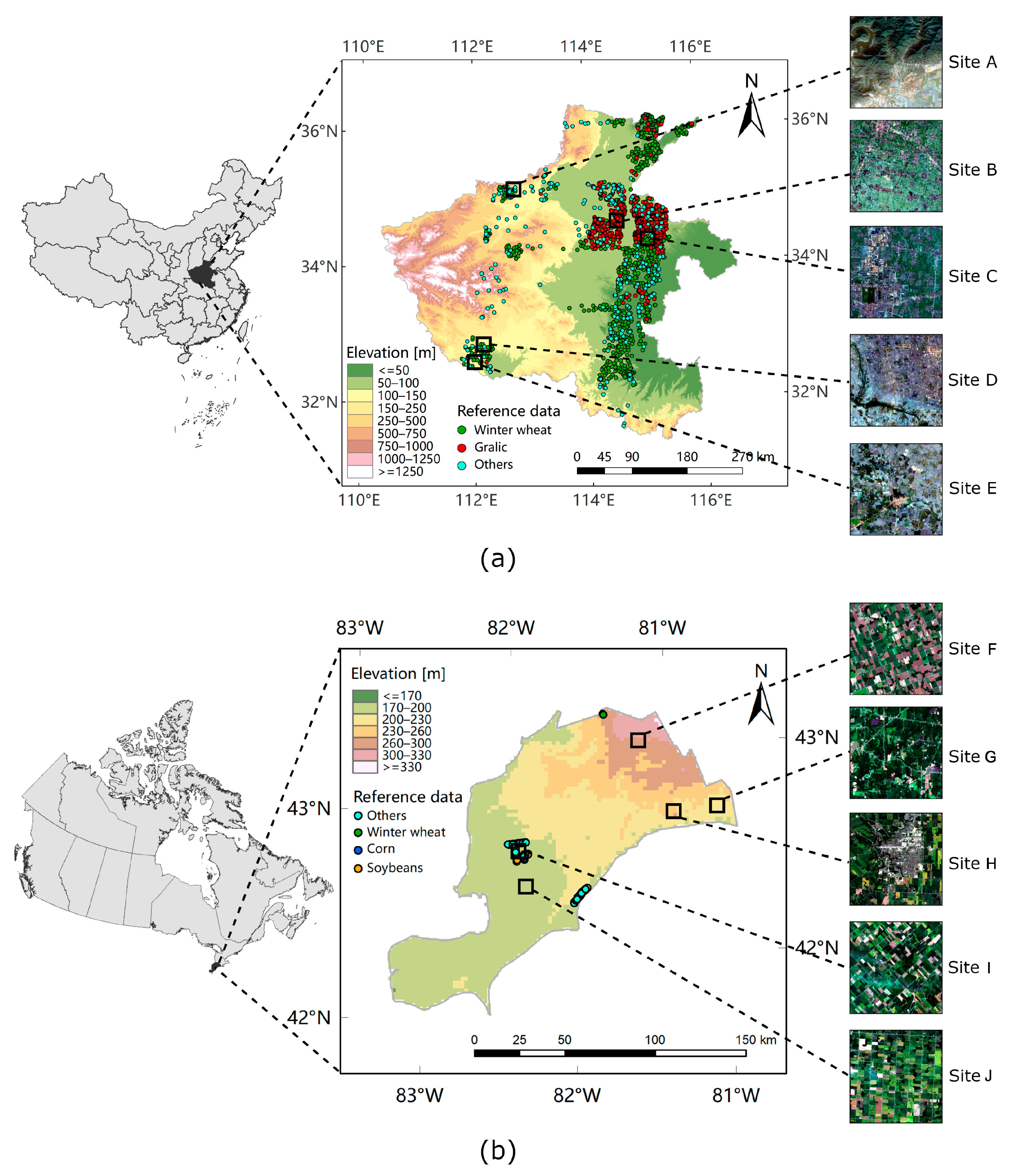
2.1. Study Areas

We chose Henan Province of China and southern Ontario of Canada as our study areas because crop parcels in these two places have different characteristics. Henan Province has climate conditions ranging from continental monsoon to warm temperate. Winter wheat and winter garlic are the main crop types in Henan. Winter wheat accounts for more than 50% of the total cultivated area within the province and contributes to approximately 25% of the national wheat production. Consequently, Henan plays an important role in Chinese food security protection. Winter wheat and winter garlic have similar phenological characteristics and are generally sown in October and harvested in late May to June of the following year. Unlike North America, most crop production in Henan is implemented by smallholder farmers, resulting in a relatively small and fragmented nature of the crop parcels, making it challenging for crop identification [13,25,26].

Southern Ontario of Canada is a part of the Mixedwood Plains Ecozone and an important crop planting region (Figure 1b). It has a temperate continental humid climate. The main crop types in this region are soybean, corn, and winter wheat [27]. Soybean and corn are usually seeded in April and May, ripened in September, and harvested in October. By contrast, winter wheat is usually seeded in autumn from October to November, matured and harvested from June to August the following year. Agriculture in North America is mainly a large-scale commercial agriculture with high levels of mechanization, leading to mostly regular-shaped and large-sized parcels [26,28].

2.2. Medium-Resolution Satellite Imagery

Given the long temporal span of Landsat satellites since 1970s and the higher spatial and temporal resolution of Sentinel-2, they are the two most widely used medium-resolution satellite imagery platforms for crop mapping [8,29]. Therefore, we selected Sentinel-2 and Landsat-8 images as the satellite data sources for our research.

Preprocessed products of Sentinel-2 and Landsat-8 are archived in the Google Earth Engine (GEE) platform, allowing users to access them conveniently and free of charge [30]. According to the sample collection time, we obtained Sentinel-2 orthorectified surface reflectance products with cloud cover lower than 10% from GEE for Henan from October 2019 to June 2020, and for southern Ontario from the entire year of 2019. Since the training data of SAM primarily comprise RGB composite images and to align with the requirements of our designed sample generation method, we utilized the red, green, blue, and near-infrared bands of Sentinel-2.

Similar to Sentinel-2 acquisition but considering the longer revisit time of Landsat-8, which is 16 days compared to 5 days of Sentinel-2, resulting in lower data availability, we derived the Landsat-8 corrected surface reflectance products with cloud cover lower than 30% from GEE covering the same periods for study areas. Red, green, blue, and near-infrared bands were also selected for experiments. All Sentinel-2 and Landsat-8 images were reorganized into 10 km × 10 km blocks [31].

2.3. Ground Truth Samples

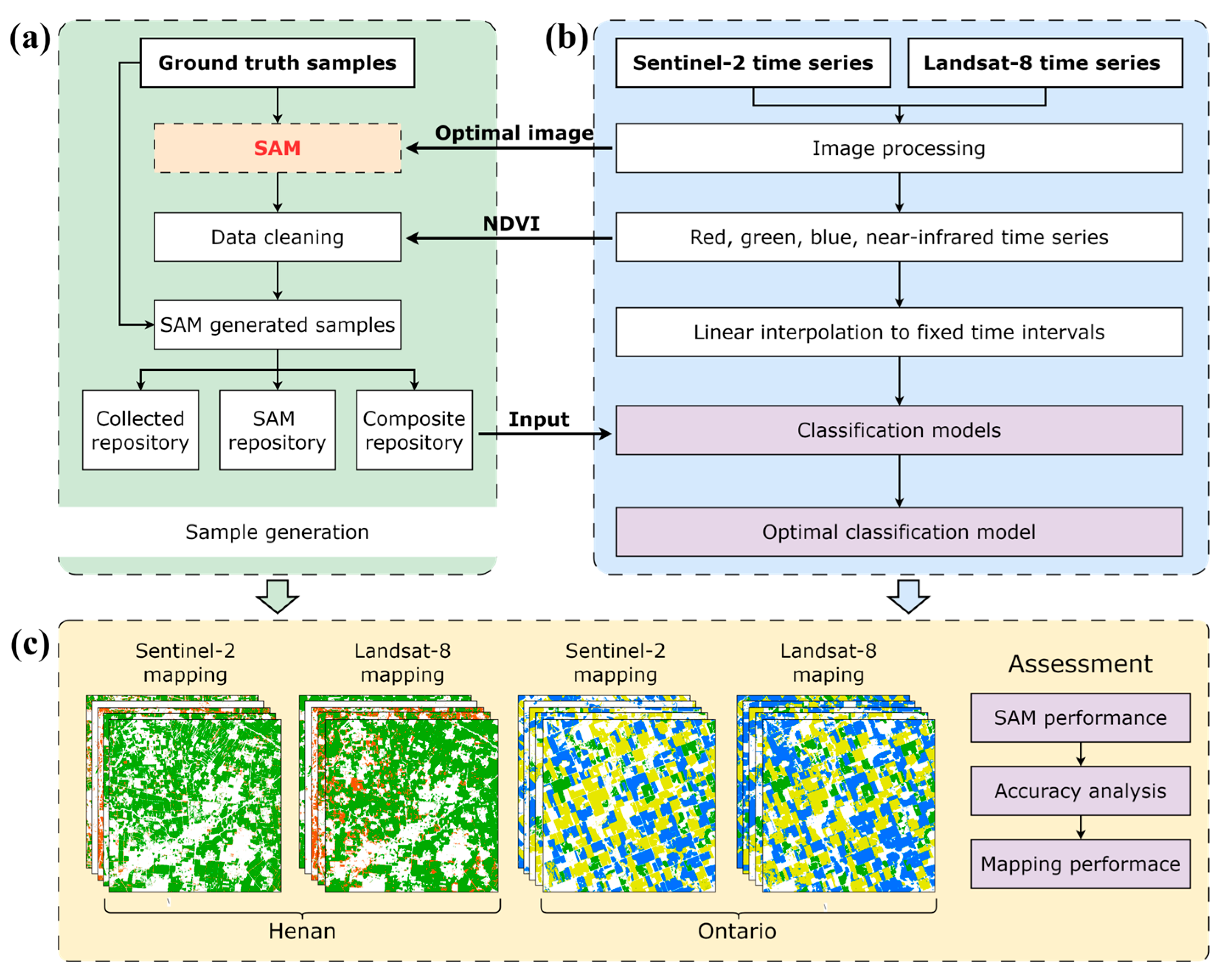
The ground truth samples used in this study for Henan were collected from 7–21 December 2019, through field surveys using global positioning system [32]. The samples included the main crop types of Henan (i.e., winter wheat and winter garlic) and other land-cover types (e.g., forests and buildings). To ensure the credibility of the samples, we performed a secondary verification for samples using visual interpretation through Google Earth. The number of final selected samples (Figure 1a) can be seen from

Table 1. The types and numbers of collected samples used in two study areas.

Study Area	Class	Numbers
Henan Province	Winter wheat	1044
	Winter garlic	860
	Others	290
Ontario	Soybean	165
	Corn	216
	Winter wheat	38
	Others	141

.

As for southern Ontario, we obtained ground truth samples in 2019 from the Annual Crop Inventory Ground Truth Data [33]. The samples are collected via crop insurance data and windshield surveys by Agriculture and Agri-Food Canada (AAFC). We selected soybean, corn, and winter wheat as three classes of interest and assigned an others label to other crops. To test the performance of our sample generation method, we only chose samples from three 10 km × 10 km blocks (Figure 1b). Ultimately, the number of samples is shown in Table 1. It is worth noting that the samples collected by AAFC do not include non-crop types such as buildings and forests. The selection of our mapping regions aims to examine the impact of this omission.

3. Methodology

This paper performed crop mapping with a novel automated sample generation method based on SAM for medium-resolution satellite imagery (Figure 2). First, a sample generation framework based on SAM was designed, including three steps: image optimization, mask production, and sample cleaning, to generate more training samples. Next, the generated samples were fed into classification models to check if they can improve the accuracy. Then, we conducted crop mapping in selected typical regions of Henan and Ontario with the trained models. The parcel segmentation performance of SAM on Sentinel-2 and Landsat-8 was analyzed. Meanwhile, the effectiveness of the proposed sampling method was demonstrated by comparing the performance of models trained on field-survey-collected samples and generated samples. The details of each component are presented in the following figure.

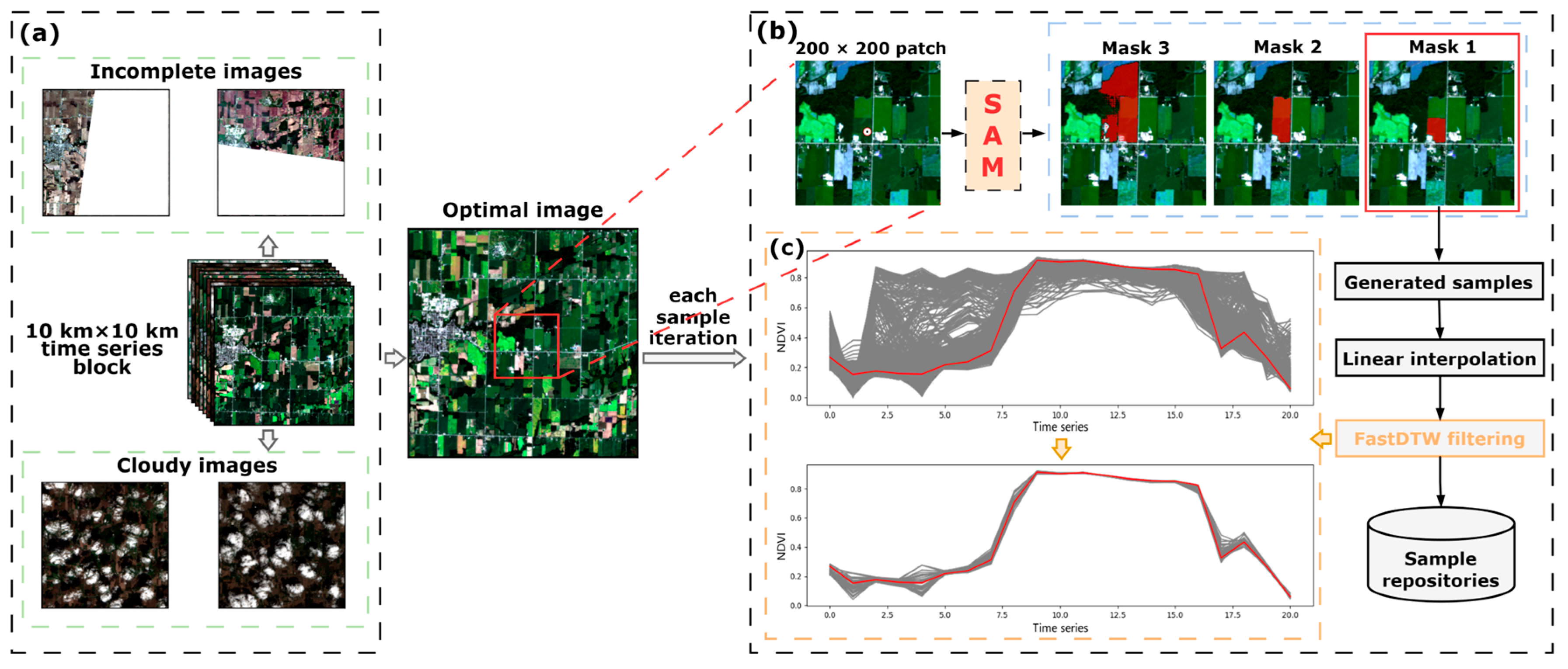
3.1. Automated Sample Generation Based on SAM

Considering the Tobler’s First Law of Geography, which indicates that the pixels within the same crop parcels are highly likely to belong to the same type of crop, this study proposed an automated sample generation framework based on SAM relying on field-survey-collected samples to generate more training samples. SAM was used for extracting the parcel where the collected sample was located. Due to few explorations of using SAM directly on medium-resolution satellite imagery, we intended to use time-series information of satellite images as auxiliary data. Therefore, we employed a variant of the Dynamic Time Warping (DTW) algorithm and a similarity index to set a threshold for filtering the potential samples, resulting in a refined set of reliable samples. The procedure of the approach is illustrated in Figure 3, and the following sections provide a thorough description.

3.1.1. Image Optimization

To automate the sample generation process, we did not tend to manually select the input image for SAM. We implemented an automated image selection within the 10 km × 10 km blocks where the samples are located. There exist incomplete images and cloudy images that cannot provide the entire parcel information (Figure 3a). If these images are inputted into SAM, the segmentation of the parcels becomes difficult. Therefore, we automatically performed statistics of cloudy and invalid pixels for all images within the block using the quality bands of Sentinel-2 and Landsat-8. Subsequently, we selected images with the least problematic pixels as the optimal images. Furthermore, considering sizes of parcels in medium-resolution imagery and computational efficiency, it is unnecessary to input the whole optimal image into SAM. Thus, we cropped a patch of 200 × 200 centered around each sample as the input to SAM (Figure 3b). If a sample is located near the boundary, the cropping range is adaptively adjusted to extract only the portion containing valid data.

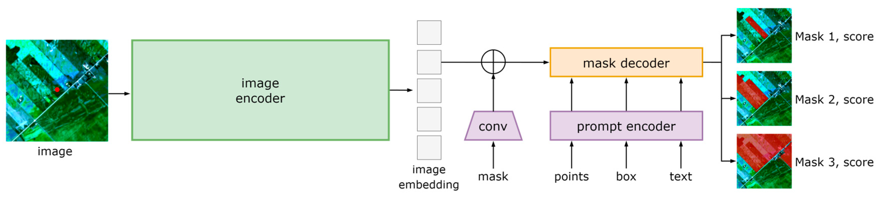
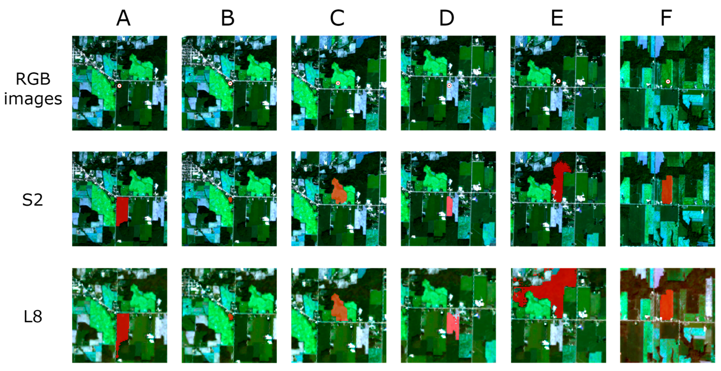
3.1.2. Mask Production

SAM is a foundation model to unify the whole image segmentation task [19]. The structure of SAM (Figure 4) mainly consists of three parts: an image encoder, a prompt encoder, and a mask decoder. The most important aspects for users are the prompt settings and the three mask outputs with confidence scores. SAM can receive points, boxes, and text forms of prompts for segmentation, among which point prompt is particularly well suited for field-survey-collected samples that contain coordinate and attribute information. Therefore, point prompt was adopted for our method. Additionally, although SAM generally outputs Masks 1–3 with increasing confidence scores, a higher score does not necessarily indicate better results in satellite image segmentation. This phenomenon is demonstrated in Section 4.1. We selected only Mask 1 as the candidate region for generating samples (Figure 3b).

3.1.3. Sample Cleaning

Based on field-survey-collected samples and SAM, we can generate parcel masks, which represent the candidate regions for potential samples. However, two reasons hinder the direct usage of these potential samples: (1) The parcel segmentation performance of SAM on medium-resolution satellite imagery is questionable and requires evaluation, leading to possible errors in masks generated. (2) Candidate regions may not only consist of the crops of interest, because there may be cultivating other types of crops. Therefore, it is important to introduce a sample cleaning approach to acquire reliable samples out of these potential samples. The time-series normalized-difference vegetation index (NDVI) is widely applied for crop sample cleaning, as it can reflect the growing trajectories and canopy characteristics of different crops [4,5]. Thus, we took the time-series NDVI extracted from all available satellite images at the field-survey sample location during each generation iteration as the reference curve for sample cleaning (Figure 3c). We chose not to use any smoothing method to preprocess the reference curve during sample cleaning. While smoothing can eliminate potential noise, it can also unintentionally remove some inherent features of the curve, and some features are quite sensitive [34]. We intended to retain the potential samples that closely resemble the reference curve of the actual sample. The gaps caused by cloud and invalid data on the timeline were filled by linear interpolation.

Some studies tended to use mean, standard deviation, and simple distance for curve similarity measuring [5,6]. However, these methods can lead to filtering out of curves that exhibit shifts due to variations in sowing time. In addition, simple distance-based methods would also lead to identification failure of the dynamic change of the tendency [35]. In this study, we adopted a variant of DTW, i.e., FastDTW [36]. DTW employs a dynamic programming approach to calculate the minimum distance between two curves. It accommodates variations in the time dimension by warping the sequences through stretching or shrinking [37]. FastDTW can execute DTW with higher efficiency, making it possible to be implemented in large scales. We defined a similarity index (SI) to set thresholds for sample cleaning according to the distance calculated by FastDTW. The SI equation is as follows:

$$SI=\frac{1}{1+\mathit{distance}}$$

(1)

SI can indicate the similarity between curves, where a value closer to 1 signifies a higher degree of similarity. Due to the lower spatial resolution of Landsat-8, the issue of mixed pixels is more pronounced. To ensure the credibility of generated samples, a higher SI is set for Landsat-8 compared to Sentinel-2. We set SI to 0.7 and 0.9 for Sentinel-2 and Landsat-8, respectively.

3.2. Classification with Generated Samples

Generating additional training samples theoretically increases the diversity of the dataset, allowing the model to learn richer features and improving its performance. We designed experiments to demonstrate that the samples generated through our method can enhance the performance of classification models.

3.2.1. Samples Division

To ensure the credibility of the experiment, it is crucial to guarantee the independence of the test set. We randomly extracted a portion of field-survey-collected samples from two study areas, in a 1:1 ratio, to form the test set (Figure 5a). The number of samples in the test set can be seen in

Table A3. Number of samples in each set and repository. Val indicates Validation.

	Class	Test Set	Collected Repository		SAM Repository		Composite Repository
			Train Set	Val Set	Train Set	Val Set	Train Set	Val Set
Henan	Winter wheat	522	417	105	6513	1628	6930	1733
	Winter garlic	430	344	86	1353	338	1697	424
	Others	145	116	29	294	74	410	103
Ontario	Soybean	82	66	17	7997	1999	8062	2016
	Corn	108	86	22	12,717	3180	12,804	3201
	Winter wheat	19	15	4	421	105	436	109
	Others	71	56	14	1405	352	1462	366

. This test set remained separate from the sample generation process and was solely utilized for evaluating the accuracy of the model. The rest of the collected samples went through the proposed sample generation method. To explore the reliability of the generated samples, we divided the rest of the collected samples and generated samples into three sample repositories. Specifically, the first repository, namely collected repository, consisted of the remaining field-survey-collected samples that were not chosen for the test set. The SAM repository only contained samples generated by our sample generation method. The third repository, composite repository, represented all samples from the above two repositories. Each repository was randomly divided into training and validation sets in a 4:1 ratio. In addition, we also sequentially randomly selected 10%, 30%, 50%, 70%, and 90% of the samples from the SAM repository and added them to the samples from the collected repository. Through observing the changes in model accuracy, we could validate the effectiveness of our method.

3.2.2. Model Establishment

To validate the reliability of the generated samples, we applied six widely used models for crop mapping, including three machine learning models: random forest (RF), support vector machine (SVM), and k-nearest neighbors (KNN), as well as three deep learning models: attention-based bidirectional long short-term memory (AtBiLSTM) [38], Conv1d-based [39], and transformer [40] (Figure 5b). It is worth noting that the focus of this study is on evaluating the parcel segmentation performance of SAM on medium-resolution satellite imagery and the effectiveness of our sample generation method, hence no tricks and parameter tuning for models were employed. Our primary concern lies in whether the samples generated by our approach can improve the accuracy and mapping performance of the models. As a result, for machine learning algorithms, we utilized the default parameters provided by the scikit-learn library [41]. As for deep learning algorithms, we referred to the parameters of the above studies, and train and validation sets were used for selecting the best model in 100 epochs, and test set for testing accuracy. All models were trained on a server of CentOS Linux 7.9 with an Intel Xeon Gold 6326 CPU and an NVIDIA A100 GPU. During the classification stage, we generated the complete time-series curves with fixed time intervals for each pixel. Specifically, we used a 5-day interval for Sentinel-2 time series and a 16-day interval for Landsat-8 time series. We used models trained on three different sample repositories to perform predictive mapping on typical regions of the study areas.

3.2.3. Accuracy Evaluation

We used the weighted-average F1 (W-F1 for short) to evaluate the performance of each model. The W-F1 assigns different weights to per-class F1 considering the actual percentage of occurrences of each class in the dataset. The W-F1 takes into account class imbalance and combines producer’s accuracy (PA) and user’s accuracy (UA), providing a comprehensive evaluation of the multiclass classification models [42,43]. Per-class F1 was used for the evaluation of each crop type. Additionally, kappa coefficient is used as a supplement [44]. The equations used for the indicators are as follows:

$$F1=\frac{2\times (PA\times UA)}{PA+UA}$$

(2)

$$Weighted-average F1={\displaystyle \sum p_k\times F{1}_k}$$

(3)

$$\mathit{Kappa} \mathit{coefficient}=\frac{p_0-p_e}{1-p_e}$$

(4)

where k denotes the type of the crop, and p indicates the number of actual occurrences of the class in the dataset. P₀ represents the proportion of correctly classified samples out of the total number of samples, while P_e denotes the expected accuracy calculated as the sum of the products of the actual and predicted sample numbers across all categories, divided by the square of the total number of samples.

4. Results

4.1. The Performance of SAM on Parcel Segmentation

By default, SAM outputs three masks in sequence (i.e., Masks 1, 2, and 3) with confidence scores, where scores give the model’s own estimation of quality. Generally, a higher score indicates a better result for natural images used in the CV community, but this may not hold true for parcel segmentation using medium-resolution satellite imagery. We selected cases of Sentinel-2 in two study areas to demonstrate this situation (Figure 6). As the score increased, the results from SAM became worse, and it may even misclassify the entire image as the target. We found that regardless of scores, the first mask outputted by SAM on medium-resolution satellite imagery, namely Mask 1, demonstrated relatively better performance because Mask 1 normally represents the subpart that is closer to the parcels where the samples are located [19]. Therefore, the mismatch between score and performance, as well as the relatively better performance of Mask 1, were the reasons for only using Mask 1 in Section 3.1.2.

Several typical patches of Mask 1 in two study areas were also chosen for further analysis. Results in Henan exhibited subpar performance both on Sentinel-2 and Landsat-8 images (Figure 7). The parcels in Figure 7A,D are relatively regular and well defined, demonstrating relatively good performance of SAM on both types of imagery. However, the performance sharply declined when the parcels were irregular or had unclear boundaries (Figure 7B,C). The results even exhibited salt-and-pepper noises, rather than being complete and connected. Moreover, the disadvantage of Landsat-8 with a lower spatial resolution was clear in Figure 7B. Field-survey samples are typically collected near roads for convenience rather than at the center of parcels. This may cause samples to shift to road pixels in coarse-resolution imagery. Consequently, the results may identify roads instead of parcels. As for buildings, the performances of SAM on Sentinel-2 and Landsat-8 were both acceptable (Figure 7E), which may be attributed to the distinct texture and color differences between buildings and the surrounding parcels.

In Ontario, the results were significantly better compared to results in Henan (Figure 8). This can be attributed to the larger and more regular parcel patterns in Ontario, which makes it easier for SAM to recognize. Figure 8A,D,F represent the results of rectangular-like parcels. It can be observed that although results on Sentinel-2 imagery consistently outperformed those on Landsat-8 imagery, SAM performed well on both Sentinel-2 and Landsat-8 images. Figure 8B,C represent small and irregular parcels in the region, respectively, and SAM also derived satisfactory results. One of the cases where SAM did not achieve satisfactory results is illustrated in Figure 8E, representing parcels adjacent to forests. The results of SAM on Sentinel-2 and Landsat-8 images both extend beyond the actual boundaries of the parcels, reaching into the adjacent forest areas.

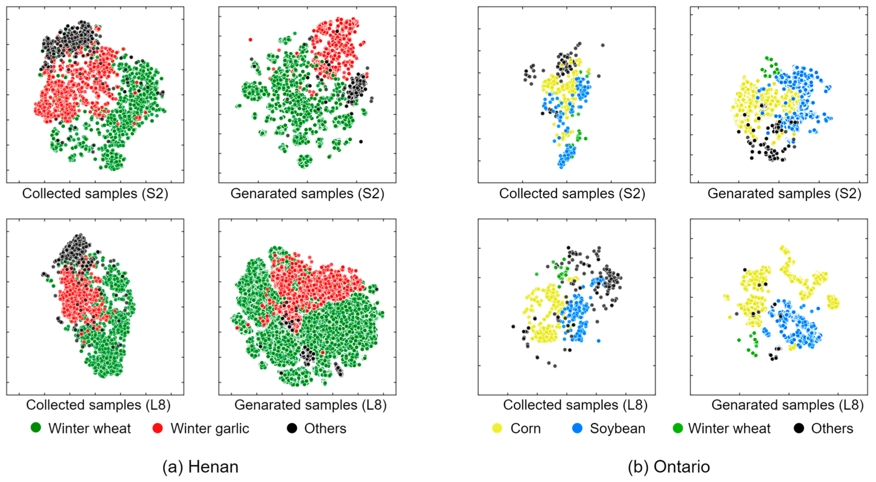
4.2. The Generated Samples and Analysis

A large number of samples in both Sentinel-2 and Landsat-8 imagery can be generated based on the proposed sample generation method (

Table 2. The types and numbers of generated samples with Sentinel-2 (S2) and Landsat-8 (L8) in two study areas.

Study Area	Class	Collected Samples	Generated Samples (S2)	Generated Samples (L8)
Henan Province	Winter wheat	522	8141	76,688
	Winter garlic	430	1691	6513
	Others	145	368	1257
Ontario	Soybean	83	9996	2881
	Corn	108	15,897	2922
	Winter wheat	19	526	452
	Others	70	1757	151

). The number of generated samples was dependent on the collected sample quantity. Compared to the collected samples, the highest number of generated samples was observed in winter wheat, with a total of 8.5 times more samples generated using Landsat-8 in Henan. Others generated the lowest number of samples both in Henan and Ontario, with 368 using Sentinel-2 and 151 using Landsat-8, respectively. While the number of generated samples for the others class was multiplied compared to its original samples, it remained significantly lower than the various crops within the same region and data source.

We also selected patches to further analyze the sample cleaning process (Figure 9 and Figure 10). Overall, our method achieved the desired objectives in both Henan and Ontario: generating training samples that are the closest to the reference samples. In addition, the comparison of the results between Figure 9, L8 and Figure 10, L8 also explains the aforementioned imbalance in the number of generated samples between Sentinel-2 and Landsat-8 in Henan and Ontario. It can be observed that the number of Landsat-8 time-series images in Henan was less than half of the quantity in Ontario. This lack of temporal information naturally posed challenges for sample cleaning.

In Henan, there were cases where no or only a few samples were generated (Figure 9A,B,E). On the one hand, we set high SI values for high demand. On the other hand, in Figure 9B, the potential samples themselves were erroneous due to the incorrect results using Landsat-8. In the case of Figure 9E, as mentioned above, buildings lack standardized time-series patterns, making it difficult to retain corresponding samples after sample cleaning. As for situations in Figure 9B,C, they aligned with our desired outcome of generating more samples based on the reference samples.

In Ontario, the results were consistent with the previous findings that Sentinel-2 outperformed Landsat-8 in sample generation. In Figure 10B represents a soybean sample, but exhibits a bimodal curve, which can be attributed to crop rotation practices. Similarly, Figure 10D represents winter wheat and shows a unimodal curve, but crop rotation can also result in bimodal curves. Such crop rotation introduces challenges and ambiguities to the representativeness of generated samples.

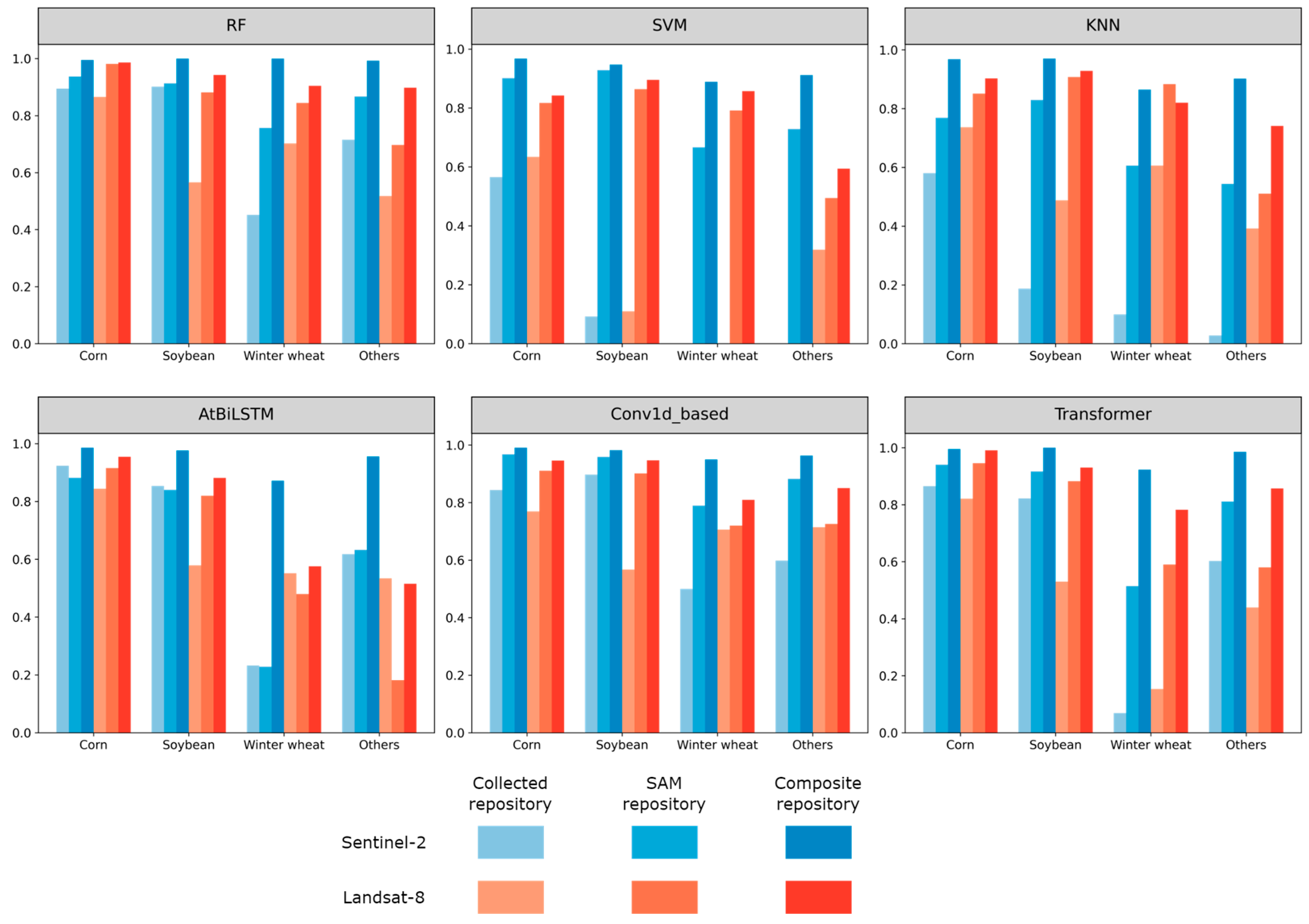
4.3. Classification with Generated Samples

We trained models by gradually adding different proportions of generated samples to the collected samples in order to validate the effectiveness of generated samples in improving accuracies (Figure 11). Overall, as the number of generated samples were continuously added, the W-F1 of all models showed a consistent improvement until reaching a stable level. For each model in two study areas, the W-F1 obtained by using Sentinel-2 was higher than that obtained by using Landsat-8 when reaching stability. The fluctuation of AtBiLSTM was more pronounced compared to other models, especially when 50% and 70% of generated samples were added. This can probably be attributed to the fact that AtBiLSTM had not reached convergence and can ingest more samples. Nevertheless, our sample generation method demonstrated a significant enhancement in accuracy compared to only using collected samples.

The W-F1 of each model trained on different repositories is shown in

Table 3. Weight-average F1 scores of classifiers on different repositories and satellite images in Henan. The bolded values indicate the best accuracy of the model across different sample repositories.

Model	Satellite	Collected Repository	SAM Repository	Composite Repository
RF	S2	0.840	0.930	0.970
	L8	0.770	0.909	0.963
SVM	S2	0.796	0.909	0.921
	L8	0.829	0.858	0.883
KNN	S2	0.722	0.868	0.917
	L8	0.831	0.868	0.904
AtBiLSTM	S2	0.843	0.793	0.904
	L8	0.783	0.853	0.859
Conv1d-based	S2	0.714	0.880	0.915
	L8	0.665	0.823	0.870
Transformer	S2	0.758	0.847	0.949
	L8	0.799	0.859	0.920

and

Table 4. Weight-average F1 scores of classifiers on different repositories and satellite images in Ontario. The bolded values indicate the best accuracy of the model across different sample repositories.

Model	Satellite	Collected Repository	SAM Repository	Composite Repository
RF	S2	0.822	0.900	0.996
	L8	0.679	0.872	0.946
SVM	S2	0.245	0.850	0.942
	L8	0.357	0.749	0.797
KNN	S2	0.293	0.720	0.945
	L8	0.568	0.785	0.865
AtBiLSTM	S2	0.780	0.763	0.968
	L8	0.668	0.674	0.797
Conv1d-based	S2	0.775	0.932	0.979
	L8	0.691	0.849	0.913
Transformer	S2	0.733	0.872	0.989
	L8	0.594	0.811	0.925

. The number of samples in each repository can be seen in Table A3. All classification models achieved significant improvement through our sample generation approach compared with only using field-survey-collected samples. Even in most cases, models trained only using generated samples achieved higher accuracy compared to models trained on collected repository. In Henan (Table 3), among experiments with composite repository, the highest W-F1 was 0.970, which was achieved via RF with Sentinel-2 images. The lowest W-F1 was acquired through AtBiLSTM with Landsat-8 images. In Ontario (Table 4), more significant results were achieved. RF with Sentinel-2 images even obtained a W-F1 of 0.996. These good results could be attributed to the relatively limited number of collected samples available in Ontario and the presence of large and regular-shaped agricultural parcels that can facilitate the performance of our sample generation method. The kappa coefficient of each model trained on different repositories can be seen in

Table A1. Kappa coefficient of classifiers on different sample repositories and satellite images in Henan. The bolded values indicate the best accuracy of the model across different sample repositories.

Model	Satellite	Collected Repository	SAM Repository	Composite Repository
RF	S2	0.735	0.884	0.950
	L8	0.608	0.842	0.936
SVM	S2	0.672	0.850	0.868
	L8	0.705	0.751	0.796
KNN	S2	0.544	0.783	0.862
	L8	0.705	0.772	0.834
AtBiLSTM	S2	0.740	0.677	0.841
	L8	0.630	0.745	0.758
Conv1d-based	S2	0.550	0.800	0.859
	L8	0.438	0.693	0.773
Transformer	S2	0.598	0.753	0.916
	L8	0.652	0.756	0.861

and

Table A2. Kappa coefficient of classifiers on different sample repositories and satellite images in Ontario. The bolded values indicate the best accuracy of the model across different sample repositories.

Model	Satellite	Collected Repository	SAM Repository	Composite Repository
RF	S2	0.751	0.857	0.995
	L8	0.525	0.831	0.923
SVM	S2	0.027	0.791	0.918
	L8	0.147	0.671	0.727
KNN	S2	0.073	0.607	0.923
	L8	0.384	0.728	0.813
AtBiLSTM	S2	0.687	0.664	0.954
	L8	0.520	0.614	0.734
Conv1d-based	S2	0.695	0.902	0.969
	L8	0.565	0.786	0.877
Transformer	S2	0.626	0.819	0.985
	L8	0.409	0.747	0.893

. The kappa coefficient and the W-F1 score illustrated similar results.

We also analyzed the relative growth achieved by the models using composite repository compared to using only the collected samples (Figure 12). In Henan, based on Sentinel-2 and Landsat-8, an average increase of 20% and 16% was achieved, respectively. The Conv1d-based model achieved the highest increase on both Sentinel-2 and Landsat-8. SVM, KNN, and transformer showed much greater increases on Sentinel-2 compared to their increases on Landsat-8. In Ontario, based on Sentinel-2 and Landsat-8, an average increase of 102% and 55% was achieved, respectively. Significant increases were observed in SVM and KNN, particularly with Sentinel-2 imagery. In comparison, AtBiLSTM showed relatively smaller increases in performance. Overall, the generated samples tended to have a larger impact on models based on Sentinel-2.

The accuracy of each model in predicting crop types was also analyzed across different repositories. In Henan (Figure 13), based on Sentinel-2 imagery, all crops achieved the best accuracy with the composite repository. Only AtBiLSTM exhibited lower accuracy in identifying winter wheat and others classes when using the SAM repository compared to the collected repository. The situation is similar for Landsat-8, as in most cases, models based on the composite repository achieved higher accuracy. In Ontario (Figure 14), most crops also demonstrated higher accuracy with the composite repository compared to the collected repository. However, the results of SVM are worth noting. The SVM model trained with the collected samples achieved W-F1 scores of 0 in the recognition test for winter wheat and others. This could also be attributed to the relatively small number of collected samples available in Ontario.

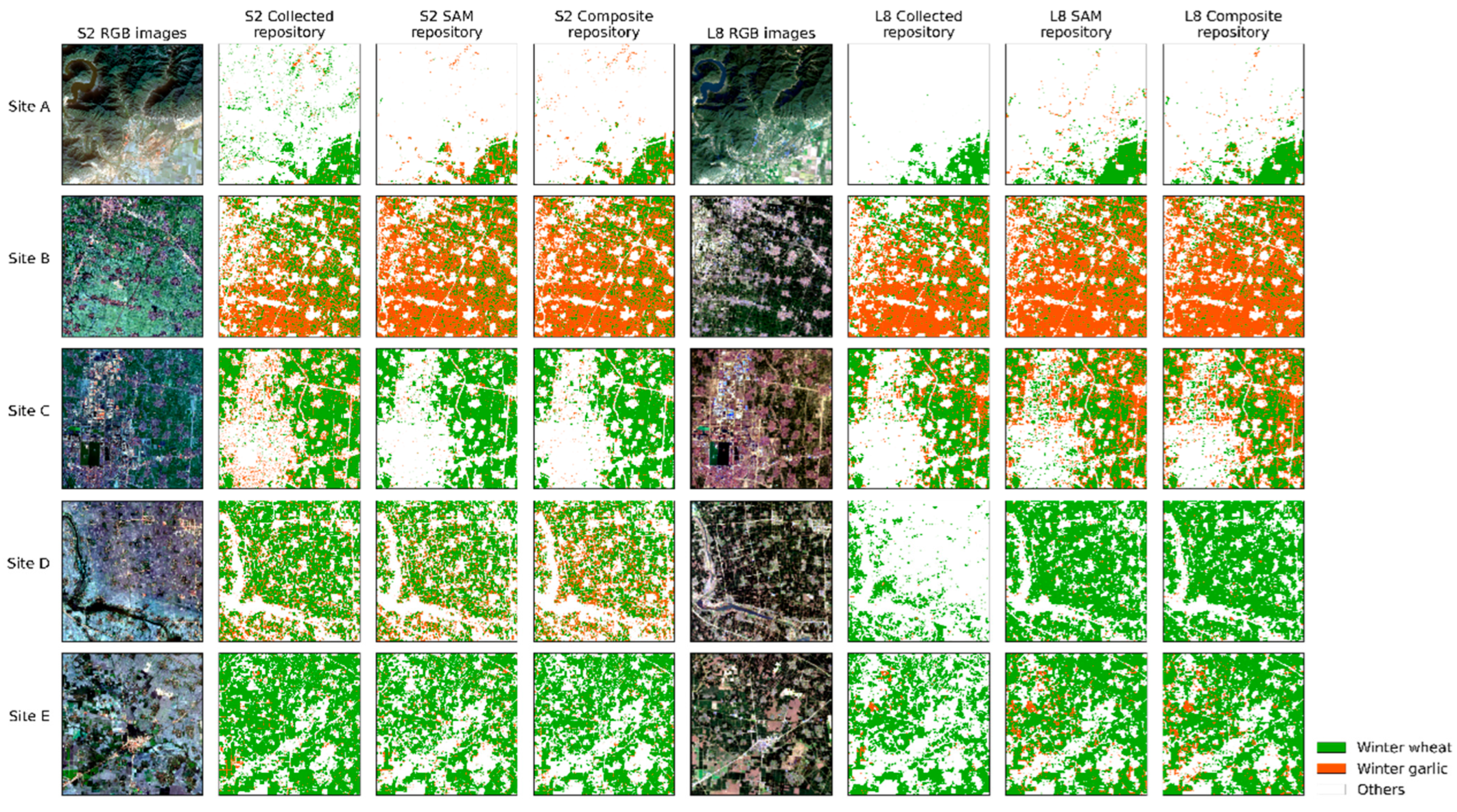
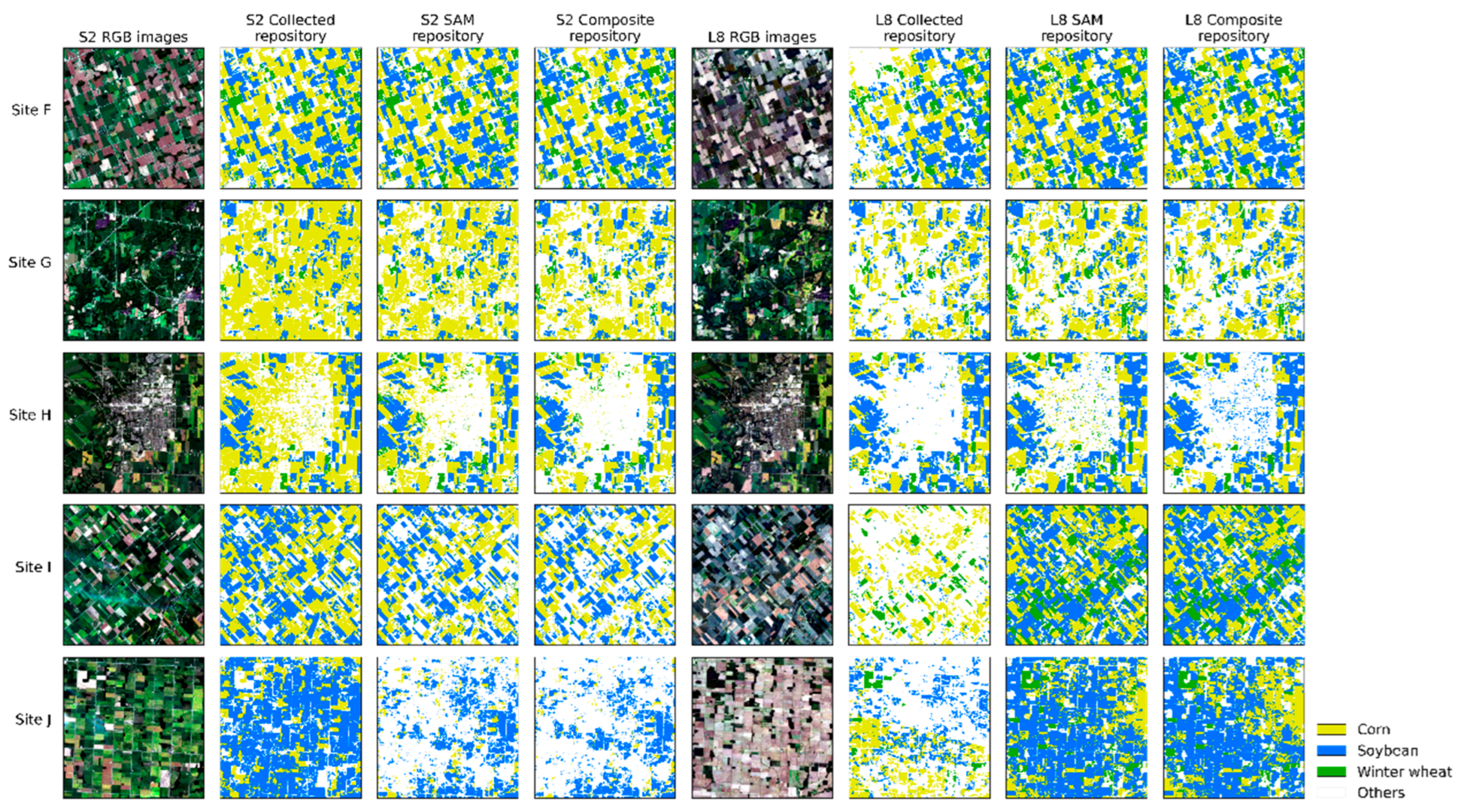
4.4. The Crop Mapping Performance Analysis

We conducted crop mapping in representative regions of Henan and Ontario using models trained on different repositories and satellite images. The results obtained from the RF model, whose numerical accuracy was relatively high, were selected for qualitative analysis. Results of other models can be found in the Supplementary Materials. In Henan (Figure 15), as more generated samples were incorporated into models, the mapping accuracy improved compared to using only the collected samples. Sites A and C represent mountainous and urban areas, respectively. In Sentinel-2 imagery, it can be observed that the misclassification of mountains and buildings as crops was reduced after incorporating the generated samples. This improvement can also be observed in Site D of Landsat-8 imagery, in that the classification of crops has been enhanced in this region. However, the performance of Sites A and C in Landsat-8 imagery was not satisfactory, as more places of mountains and buildings were misclassified as crops with the injection of generated samples. This could be attributed to the coarser spatial resolution of Landsat-8, which is not conducive to the application in areas like Henan with small and fragmented crop parcels.

In Ontario (Figure 16), due to larger and more regular parcels, the mapping performance was better, and there was also an improvement in mapping with the injection of generated samples. In Sites G and H of Sentinel-2, when using the collected repository, RF reduced the misclassification of buildings and forests as crops. Considering that the collected samples in Ontario do not inherently include buildings and forests, this improvement is significant. However, Site J showed a relatively poor performance. In Landsat-8, although the mapping performance was improved in Sites F, G, I, and J, similar to the situation in Henan, there was an increase in the misclassification of buildings as crops with the injection of generated samples (Figure 16, Site H). This misclassification is probably not due to the samples themselves but rather the missing crucial temporal information in the regional images because a number of images were filtered out when considering the cloud cover factor in the beginning.

5. Discussion

5.1. The Capability of SAM on Medium-Resolution Satellite Imagery

This study analyzed the parcel segmentation capability of SAM on medium-resolution satellite imagery (Sentinel-2 and Landsat-8) in two study areas with different characteristics of parcels. For small and fragmented parcels in Henan, SAM performed poorly, struggling to achieve accurate results with well-defined boundaries even on Sentinel-2 with its higher spatial resolution, not to mention Landsat-8 imagery. It exhibited difficulties in accurately identifying the target parcels, and the results often spilled over to surrounding areas. Moreover, the results occasionally contained salt-and-pepper noises. In Ontario with large and regular parcels, although the results by SAM on both Sentinel-2 and Landsat-8 were significantly better than those in Henan, issues persisted. Errors occurred when the target parcels had small color and texture differences with surrounding objects (such as forests), which was more obvious when using Landsat-8 images. Furthermore, SAM showed a relatively better performance in urban areas compared to crop parcels, possibly due to more distinct color differences between urban areas and surrounding farmland.

In summary, the parcel segmentation capability of SAM on medium-resolution satellite imagery is influenced by the size, shape, and color differences of parcels with respect to surrounding objects. Directly applying SAM is feasible when the parcels have regular shapes, exhibit significant color differences from their surroundings, and are large enough to occupy a number of pixels in the imagery. However, it may fail to accurately segment when the parcels are small or have similar colors to surrounding objects, such as green forests. SAM showed better performance on Sentinel-2 compared to Landsat-8. This is expected since Landsat-8, with its coarser spatial resolution, suffers more from mixed-pixel issue.

5.2. The Effectiveness of the Proposed Sample Generation Method

The number of generated samples and optimal accuracy achieved by all classification models trained with generated samples revealed the effectiveness of the proposed sample generation approach for crop mapping. Two main factors ensured this effectiveness: location and temporal information. Based on the reference sample locations, though the segmentation performance of SAM on medium-resolution satellite imagery is variable, the mask generated by SAM can cover regions that are highly likely to belong to the same crop type as the sample. Additionally, the temporal information of the reference sample serves as a strong constraint to ensure that the latent samples left after filtering are reliable. To further prove the quality of generated samples, we used t-distributed stochastic neighbor embedding (t-SNE) to visualize the field-survey-collected samples and generated samples (Figure 17). It is obvious that the generated samples exhibit clear separability, facilitating the classification model to derive boundaries distinguishing different crop types on the hyperplane, consistent with the performance improvements shown in Table 3 and Table 4. This advantage is particularly pronounced in Ontario. The limited and potentially unrepresentative nature of collected samples leads to poor separability, whereas the generated samples effectively address this issue.

Although a large number of reliable crop samples were successfully produced across different study areas and satellite images, it can be observed from Table 2 that the quantity of samples generated for the others class is relatively low. This is reasonable because, in Henan, the others class primarily consisted of buildings, which generally have complex spectra and no standard temporal patterns, so they were filtered out by sample cleaning. On the other hand, in Ontario, the crops in the others class were minorities, making quantities inherently low. Additionally, an evident observation is that, in Henan, even though a larger SI was set for Landsat-8, the number of samples generated for each category using Sentinel-2 was lower than that generated using Landsat-8. However, in Ontario, the situation is reversed. We believed this is related to the spatial resolution and varying characteristics of agricultural parcels in study areas. In Henan, parcels are small and fragmented, and the coarser spatial resolution of Landsat-8 exacerbates the mixed-pixel problem. This not only could result in poorer performance of SAM but also lead to more pixels and more phonologically similar or same crops being included in the sample cleaning stage. However, in Ontario, agricultural parcels are predominantly large and regular, which can enable SAM to achieve more accurate results using Landsat-8. This reduced the inclusion of unnecessary pixels in the sample cleaning stage. The higher spatial resolution of Sentinel-2 naturally leads to more pixels within the same parcel, leading to the generation of a greater number of samples. In general, our experiments demonstrated the applicability of our sample generation method across different areas and satellite images.

It should be noted that our method has achieved good results relying on the collected samples, and it has the potential to generate more samples with less effort over large areas and multiple years. However, to ensure the effectiveness of actual predictions, we recommend collecting representative samples that are spatially evenly distributed and diverse in terms of crop types to mitigate spatial heterogeneity. Moreover, all models used in this study were not subjected to targeted hyperparameter tuning or feature engineering, and thus there are potential ways to further improve the classification accuracy.

5.3. Contributions and Future Work

SAM, a foundation model for segmentation tasks in the CV community, has gained increasing attention. Though some researchers have studied the performance of SAM on remote sensing images, their focus has mainly been on high spatial resolution imagery, even reaching submeter resolution [21,24]. This study primarily focused on investigating the parcel segmentation performance of SAM on Sentinel-2 and Landsat-8 imagery. Our results indicated that SAM’s performance on Sentinel-2 and Landsat-8 is still not satisfactory, unless the target parcels are sufficiently large, regular in shape, and have distinct color differences from the surrounding areas. However, the limited capability does not imply its inability to assist in applications involving medium-resolution satellite imagery. On the one hand, as foundation models continue to be upgraded and iterated upon, their performance is expected to improve. On the other hand, these foundation models, because of their generalization abilities, can be incorporated as part of a framework and applied to various domains. Therefore, based on SAM, this study designed an automated sample generation method and derived satisfactory results. This study provides insights and a reference for the application of foundation models in the field of remote sensing.

This study has several limitations that warrant further investigation. Firstly, although a method for automatically selecting the optimal image has been used to choose the input for SAM, the image with low cloud cover and few invalid values may not necessarily be the best input to SAM for parcel segmentation. The acquiring time of selected optimal image may coincide with the time when the parcel and surrounding areas have similar color tones, posing a challenge for SAM. We will subsequently investigate the impact of different image acquisition times on SAM’s segmentation of crop parcels. Secondly, the issue of cloud cover in optical satellite imagery may result in the loss of temporal information, which can pose difficulties in the filtering process based on time series using FastDTW and any other filtering approaches. We will consider incorporating weather-independent synthetic aperture radar (SAR) imagery for our future research. Thirdly, the segmentation capability of SAM on medium-resolution satellite imagery for crop parcels is limited, constraining its further application. In future research, we will consider conducting fine-tuning studies on SAM to improve its performance. Finally, although the results of this study demonstrated that the accuracy improves as generated samples are progressively added into model training (Figure 11), the ultimate accuracy converges to a stable level. The determination of the requisite number and characteristics of samples to achieve this stable level in practical mapping tasks still relies on experience, necessitating further comprehensive research to establish a set of standards [13].

6. Conclusions

In this study, we evaluated the parcel segmentation performance of SAM on medium-resolution satellite imagery (Sentinel-2 and Landsat-8) and designed a novel sample generation framework based on point-prompt SAM to solve the sample scarcity problem in crop mapping task and to improve the performance of crop mapping. Experiments were conducted to validate the effectiveness of the proposed approach with different study areas, sensors, crop types, and classifiers. Our results indicated that the parcel segmentation performance of SAM on medium-resolution satellite imagery is still challenging, unless the parcels are large, regular in shape, and have distinct color differences with the surroundings. The proposed method could generate a large number of high-quality training samples. The improvements achieved by each classifier demonstrated that our approach can significantly enhance the performance of crop mapping. This study explored potential applications of foundation models in crop mapping, providing valuable insights for associated studies and applications.

References

1. Blickensdörfer, L.; Schwieder, M.; Pflugmacher, D.; Nendel, C.; Erasmi, S.; Hostert, P. Mapping of crop types and crop sequences with combined time series of Sentinel-1, Sentinel-2 and Landsat 8 data for Germany. Remote Sens. Environ. 2022, 269, 112831. [Google Scholar] [CrossRef]
2. Karthikeyan, L.; Chawla, I.; Mishra, A.K. A review of remote sensing applications in agriculture for food security: Crop growth and yield, irrigation, and crop losses. J. Hydrol. 2020, 586, 124905. [Google Scholar] [CrossRef]
3. Turkoglu, M.O.; D’Aronco, S.; Perich, G.; Liebisch, F.; Streit, C.; Schindler, K.; Wegner, J.D. Crop mapping from image time series: Deep learning with multi-scale label hierarchies. Remote Sens. Environ. 2021, 264, 112603. [Google Scholar] [CrossRef]
4. You, N.; Dong, J.; Huang, J.; Du, G.; Zhang, G.; He, Y.; Yang, T.; Di, Y.; Xiao, X. The 10-m crop type maps in Northeast China during 2017–2019. Sci. Data 2021, 8, 41. [Google Scholar] [CrossRef] [PubMed]
5. Xuan, F.; Dong, Y.; Li, J.; Li, X.; Su, W.; Huang, X.; Huang, J.; Xie, Z.; Li, Z.; Liu, H. Mapping crop type in Northeast China during 2013–2021 using automatic sampling and tile-based image classification. Int. J. Appl. Earth Obs. Geoinf. 2023, 117, 103178. [Google Scholar] [CrossRef]
6. Wen, Y.; Li, X.; Mu, H.; Zhong, L.; Chen, H.; Zeng, Y.; Miao, S.; Su, W.; Gong, P.; Li, B. Mapping corn dynamics using limited but representative samples with adaptive strategies. ISPRS J. Photogramm. Remote Sens. 2022, 190, 252–266. [Google Scholar] [CrossRef]
7. Huang, H.; Wang, J.; Liu, C.; Liang, L.; Li, C.; Gong, P. The migration of training samples towards dynamic global land cover mapping. ISPRS J. Photogramm. Remote Sens. 2020, 161, 27–36. [Google Scholar] [CrossRef]
8. Tran, K.H.; Zhang, H.K.; McMaine, J.T.; Zhang, X.; Luo, D. 10 m crop type mapping using Sentinel-2 reflectance and 30 m cropland data layer product. Int. J. Appl. Earth Obs. Geoinf. 2022, 107, 102692. [Google Scholar] [CrossRef]
9. Hao, P.; Di, L.; Zhang, C.; Guo, L. Transfer Learning for Crop classification with Cropland Data Layer data (CDL) as training samples. Sci. Total Environ. 2020, 733, 138869. [Google Scholar] [CrossRef]
10. Jiang, D.; Chen, S.; Useya, J.; Cao, L.; Lu, T. Crop mapping using the historical crop data layer and deep neural networks: A case study in jilin province, china. Sensors 2022, 22, 5853. [Google Scholar] [CrossRef]
11. Boryan, C.; Yang, Z.; Mueller, R.; Craig, M. Monitoring US agriculture: The US department of agriculture, national agricultural statistics service, cropland data layer program. Geocarto Int. 2011, 26, 341–358. [Google Scholar] [CrossRef]
12. Zhang, L.; Liu, Z.; Liu, D.; Xiong, Q.; Yang, N.; Ren, T.; Zhang, C.; Zhang, X.; Li, S. Crop mapping based on historical samples and new training samples generation in Heilongjiang Province, China. Sustainability 2019, 11, 5052. [Google Scholar] [CrossRef]
13. Yu, Q.; Duan, Y.; Wu, Q.; Liu, Y.; Wen, C.; Qian, J.; Song, Q.; Li, W.; Sun, J.; Wu, W. An interactive and iterative method for crop mapping through crowdsourcing optimized field samples. Int. J. Appl. Earth Obs. Geoinf. 2023, 122, 103409. [Google Scholar] [CrossRef]
14. Tobler, W. On the first law of geography: A reply. Ann. Assoc. Am. Geogr. 2004, 94, 304–310. [Google Scholar] [CrossRef]
15. Liu, Z.; Zhang, L.; Yu, Y.; Xi, X.; Ren, T.; Zhao, Y.; Zhu, D.; Zhu, A.-X. Cross-year reuse of historical samples for crop mapping based on environmental similarity. Front. Plant Sci. 2022, 12, 761148. [Google Scholar] [CrossRef] [PubMed]
16. Zhou, Y.N.; Luo, J.; Feng, L.; Yang, Y.; Chen, Y.; Wu, W. Long-short-term-memory-based crop classification using high-resolution optical images and multi-temporal SAR data. GISci. Remote Sens. 2019, 56, 1170–1191. [Google Scholar] [CrossRef]
17. Labib, S.; Harris, A. The potentials of Sentinel-2 and LandSat-8 data in green infrastructure extraction, using object based image analysis (OBIA) method. Eur. J. Remote Sens. 2018, 51, 231–240. [Google Scholar] [CrossRef]
18. Gui, B.; Bhardwaj, A.; Sam, L. Evaluating the Efficacy of Segment Anything Model for Delineating Agriculture and Urban Green Spaces in Multiresolution Aerial and Spaceborne Remote Sensing Images. Remote Sens. 2024, 16, 414. [Google Scholar] [CrossRef]
19. Kirillov, A.; Mintun, E.; Ravi, N.; Mao, H.; Rolland, C.; Gustafson, L.; Xiao, T.; Whitehead, S.; Berg, A.C.; Lo, W.-Y. Segment anything. arXiv 2023, arXiv:2304.02643. [Google Scholar]
20. Sun, W.; Liu, Z.; Zhang, Y.; Zhong, Y.; Barnes, N. An Alternative to WSSS? An Empirical Study of the Segment Anything Model (SAM) on Weakly-Supervised Semantic Segmentation Problems. arXiv 2023, arXiv:2305.01586. [Google Scholar]
21. Wang, D.; Zhang, J.; Du, B.; Tao, D.; Zhang, L. Scaling-up remote sensing segmentation dataset with segment anything model. arXiv 2023, arXiv:2305.02034. [Google Scholar]
22. Chen, K.; Liu, C.; Chen, H.; Zhang, H.; Li, W.; Zou, Z.; Shi, Z. RSPrompter: Learning to prompt for remote sensing instance segmentation based on visual foundation model. IEEE Trans. Geosci. Remote Sens. 2024, 62, 4701117. [Google Scholar] [CrossRef]
23. Ji, W.; Li, J.; Bi, Q.; Li, W.; Cheng, L. Segment anything is not always perfect: An investigation of sam on different real-world applications. arXiv 2023, arXiv:2304.05750. [Google Scholar] [CrossRef]
24. Osco, L.P.; Wu, Q.; de Lemos, E.L.; Gonçalves, W.N.; Ramos, A.P.M.; Li, J.; Junior, J.M. The segment anything model (sam) for remote sensing applications: From zero to one shot. Int. J. Appl. Earth Obs. Geoinf. 2023, 124, 103540. [Google Scholar] [CrossRef]
25. Luo, L.; Qin, L.; Wang, Y.; Wang, Q. Environmentally-friendly agricultural practices and their acceptance by smallholder farmers in China—A case study in Xinxiang County, Henan Province. Sci. Total Environ. 2016, 571, 737–743. [Google Scholar] [CrossRef]
26. Johansen, C.; Haque, M.; Bell, R.; Thierfelder, C.; Esdaile, R. Conservation agriculture for small holder rainfed farming: Opportunities and constraints of new mechanized seeding systems. Field Crops Res. 2012, 132, 18–32. [Google Scholar] [CrossRef]
27. Laamrani, A.; Berg, A.A.; Voroney, P.; Feilhauer, H.; Blackburn, L.; March, M.; Dao, P.D.; He, Y.; Martin, R.C. Ensemble identification of spectral bands related to soil organic carbon levels over an agricultural field in Southern Ontario, Canada. Remote Sens. 2019, 11, 1298. [Google Scholar] [CrossRef]
28. Yan, L.; Roy, D.P. Conterminous United States crop field size quantification from multi-temporal Landsat data. Remote Sens. Environ. 2016, 172, 67–86. [Google Scholar] [CrossRef]
29. Qiu, B.; Lu, D.; Tang, Z.; Chen, C.; Zou, F. Automatic and adaptive paddy rice mapping using Landsat images: Case study in Songnen Plain in Northeast China. Sci. Total Environ. 2017, 598, 581–592. [Google Scholar] [CrossRef]
30. Gorelick, N.; Hancher, M.; Dixon, M.; Ilyushchenko, S.; Thau, D.; Moore, R. Google Earth Engine: Planetary-scale geospatial analysis for everyone. Remote Sens. Environ. 2017, 202, 18–27. [Google Scholar] [CrossRef]
31. Ye, S.; Liu, D.; Yao, X.; Tang, H.; Xiong, Q.; Zhuo, W.; Du, Z.; Huang, J.; Su, W.; Shen, S. RDCRMG: A raster dataset clean & reconstitution multi-grid architecture for remote sensing monitoring of vegetation dryness. Remote Sens. 2018, 10, 1376. [Google Scholar] [CrossRef]
32. Huang, X.; Huang, J.; Li, X.; Shen, Q.; Chen, Z. Early mapping of winter wheat in Henan province of China using time series of Sentinel-2 data. GISci. Remote Sens. 2022, 59, 1534–1549. [Google Scholar] [CrossRef]
33. Fisette, T.; Davidson, A.; Daneshfar, B.; Rollin, P.; Aly, Z.; Campbell, L. Annual space-based crop inventory for Canada: 2009–2014. In Proceedings of the 2014 IEEE Geoscience and Remote Sensing Symposium, Quebec City, QC, Canada, 13–18 July 2014; pp. 5095–5098. [Google Scholar]
34. Jensen, J.R. Remote Sensing of the Environment: An Earth Resource Perspective 2/e; Pearson Education: Noida, India, 2009. [Google Scholar]
35. Dong, X.-L.; Gu, C.-K.; Wang, Z.-O. Research on shape-based time series similarity measure. In Proceedings of the 2006 International Conference on Machine Learning and Cybernetics, Dalian, China, 13–16 August 2006; pp. 1253–1258. [Google Scholar]
36. Salvador, S.; Chan, P. Toward accurate dynamic time warping in linear time and space. Intell. Data Anal. 2007, 11, 561–580. [Google Scholar] [CrossRef]
37. Jeong, Y.-S.; Jeong, M.K.; Omitaomu, O.A. Weighted dynamic time warping for time series classification. Pattern Recognit. 2011, 44, 2231–2240. [Google Scholar] [CrossRef]
38. Xu, J.; Zhu, Y.; Zhong, R.; Lin, Z.; Xu, J.; Jiang, H.; Huang, J.; Li, H.; Lin, T. DeepCropMapping: A multi-temporal deep learning approach with improved spatial generalizability for dynamic corn and soybean mapping. Remote Sens. Environ. 2020, 247, 111946. [Google Scholar] [CrossRef]
39. Zhong, L.; Hu, L.; Zhou, H. Deep learning based multi-temporal crop classification. Remote Sens. Environ. 2019, 221, 430–443. [Google Scholar] [CrossRef]
40. Rußwurm, M.; Lefèvre, S.; Körner, M. Breizhcrops: A satellite time series dataset for crop type identification. Int. Arch. Photogramm. Remote Sens. Spat. Inf. Sci. 2020, XLIII-B2-2020, 1545–1551. [Google Scholar] [CrossRef]
41. Pedregosa, F.; Varoquaux, G.; Gramfort, A.; Michel, V.; Thirion, B.; Grisel, O.; Blondel, M.; Prettenhofer, P.; Weiss, R.; Dubourg, V. Scikit-learn: Machine learning in Python. J. Mach. Learn. Res. 2011, 12, 2825–2830. [Google Scholar]
42. Wang, X.; Zhang, J.; Xun, L.; Wang, J.; Wu, Z.; Henchiri, M.; Zhang, S.; Zhang, S.; Bai, Y.; Yang, S. Evaluating the effectiveness of machine learning and deep learning models combined time-series satellite data for multiple crop types classification over a large-scale region. Remote Sens. 2022, 14, 2341. [Google Scholar] [CrossRef]
43. Nowakowski, A.; Mrziglod, J.; Spiller, D.; Bonifacio, R.; Ferrari, I.; Mathieu, P.P.; Garcia-Herranz, M.; Kim, D.-H. Crop type mapping by using transfer learning. Int. J. Appl. Earth Obs. Geoinf. 2021, 98, 102313. [Google Scholar] [CrossRef]
44. Zhan, W.; Luo, F.; Luo, H.; Li, J.; Wu, Y.; Yin, Z.; Wu, Y.; Wu, P. Time-Series-Based Spatiotemporal Fusion Network for Improving Crop Type Mapping. Remote Sens. 2024, 16, 235. [Google Scholar] [CrossRef]
Figure 1. Study areas and collected samples distributions. (a) Henan Province of China, Sites A–E indicates selected regions for mapping validation. Site A represents mountainous regions. Sites B, E represent regions dominated by crops. Sites C, D exhibit interference from buildings and rivers. (b) Southern Ontario of Canada, Sites F–J indicate selected regions for mapping validation. Sites G, J, I involve disturbances like forests. Sites F, J contain uniformly shaped parcels and a wide distribution of crops.
Remotesensing 16 01505 g001
Figure 2. The overview of the whole workflow of this study. (a) Sample generation process based on SAM. (b) Image processing and model training processes. (c) Crop mapping and performance analysis.
Remotesensing 16 01505 g002
Figure 3. The procedure of the proposed sample generation method based on SAM. (a) Select an optimal image as the SAM input. (b) The process of generating potential samples and cleaning. Red color in each patch indicates the mask produced by SAM. (c) An example of corn sample in southern Ontario that demonstrates the performance of FastDTW for filtering. The red line denotes the curve of reference ground truth sample.
Remotesensing 16 01505 g003
Figure 4. The overall structure of the Segment Anything Model, adapted from Kirillov et al. [19]. The red dot indicates the point prompt for the target parcel, and the red color in the masks indicates the SAM’s results.
Remotesensing 16 01505 g004
Figure 5. The demonstration of the classification process. (a) Sample division that divides samples into a test set and three repositories. (b) Classification models used in this study.
Remotesensing 16 01505 g005
Figure 6. The outputs of SAM with confidence scores using Sentinel-2 images in Henan and Ontario. The first column in (a,b) represents RGB composite images of Sentinel-2. The second to fourth columns represent the masks outputted by SAM with scores. Green regions in (a) and red regions in (b) denote the mask produced by SAM.
Remotesensing 16 01505 g006
Figure 7. Typical cases of SAM in Henan. (AF) indicates the patches chosen for further analysis. S2 indicates results based on Sentinel-2 images. L8 indicates results based on Landsat-8 images. Green regions denote the mask produced by SAM.
Remotesensing 16 01505 g007
Figure 8. A few typical cases of SAM in Ontario. (AF) indicates the patches chosen for further analysis. S2 indicates results based on Sentinel-2 images. L8 indicates results based on Landsat-8 images. Red regions denote the mask produced by SAM.
Remotesensing 16 01505 g008
Figure 9. Demonstration of the sample cleaning method based on FastDTW in Henan. (AE) indicates the patches chosen for further analysis, corresponding to Figure 7. S2 indicates results based on Sentinel-2 images. L8 indicates results based on Landsat-8 images. Green regions denote the mask produced by SAM. The red line denotes the curve of reference sample.
Remotesensing 16 01505 g009
Figure 10. Demonstration of the sample cleaning method based on FastDTW in Ontario. (AE) indicates the patches chosen for further analysis, corresponding to Figure 8. S2 indicates results based on Sentinel-2 images. L8 indicates results based on Landsat-8 images. Red regions denote the mask produced by SAM. The red line denotes the curve of reference sample.
Remotesensing 16 01505 g010
Figure 11. Changes of weighted-average F1 with increasing number of generated samples adding to the collected samples in each model.
Remotesensing 16 01505 g011
Figure 12. The relative growth of the models using composite samples compared to only using the collected samples.
Remotesensing 16 01505 g012
Figure 13. The F1 scores of each crop under different models trained using different sample repositories and satellite images in Henan.
Remotesensing 16 01505 g013
Figure 14. The F1 scores of each crop under different models trained using different sample repositories and satellite images in Ontario.
Remotesensing 16 01505 g014
Figure 15. Crop mapping results of RF models trained on different sample repositories and satellite images in Henan.
Remotesensing 16 01505 g015
Figure 16. Crop mapping results of RF models trained on different sample repositories and satellite images in Ontario.
Remotesensing 16 01505 g016
Figure 17. Visualization of samples based on t-SNE. The time-series spectral features were nonlinearly projected to two primary dimensions. S2 indicates samples derived from Sentinel-2 imagery, L8 indicates samples derived from Landsat-8 imagery.
Remotesensing 16 01505 g017