Using the Surface Reflectance MODIS Terra Product to Estimate Turbidity in Tampa Bay, Florida

Abstract
:
1. Introduction
2. Methods
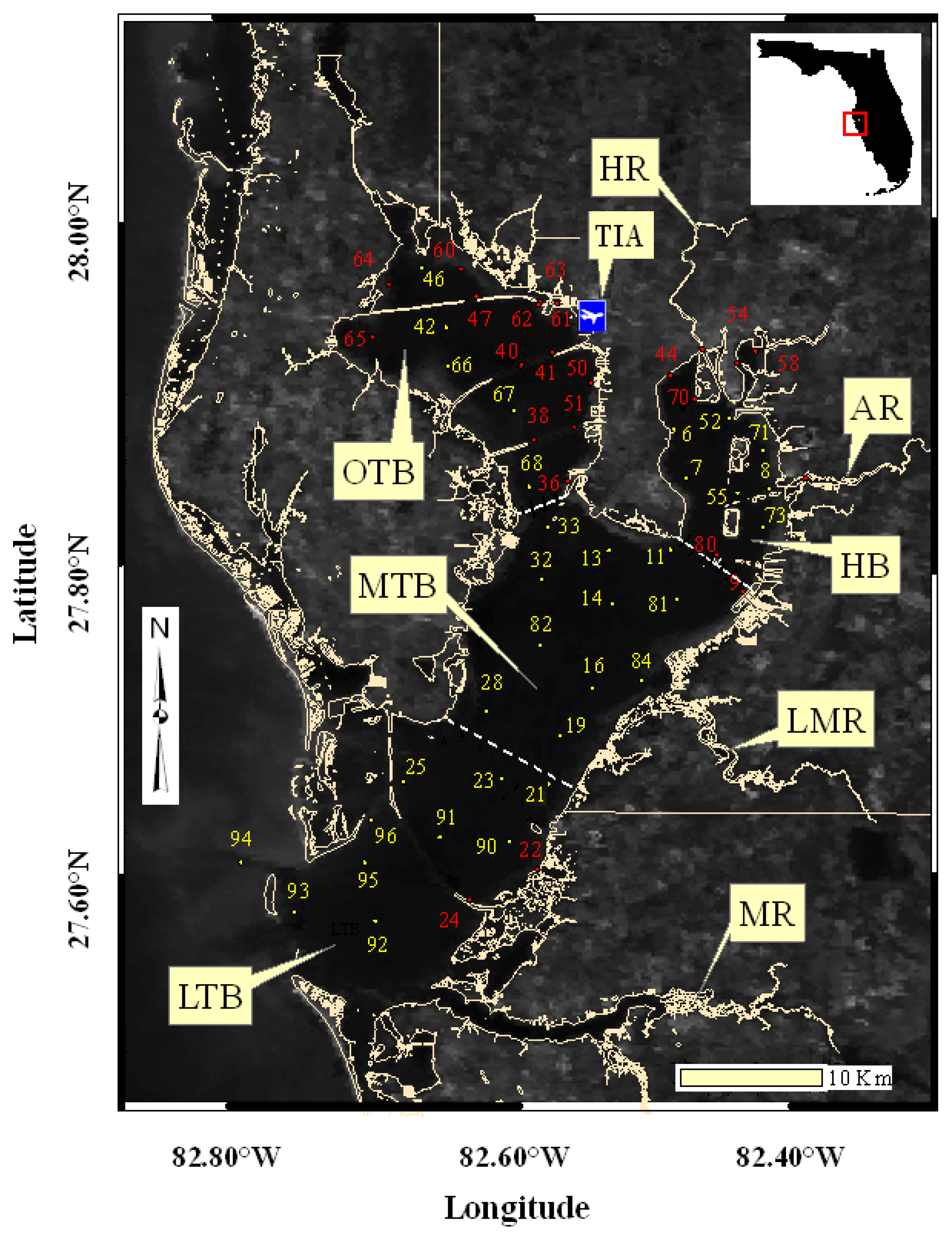
2.1. Study Area
2.2. In situ Measurements

| Depth in meters | R2 | Equation | n |
|---|---|---|---|
| 9.4 | 0.31 | 111.64 × Rrs + 1.5235 | 16 |
| 8.4 | 0.11 | 70.439 × Rrs + 2.257 | 52 |
| 7.4 | 0.19 | 107.97 × Rrs + 1.9461 | 78 |
| 6.4 | 0.17 | 107.07 × Rrs + 2.0427 | 104 |
| 5.4 | 0.17 | 120.26 × Rrs + 2.041 | 144 |
| 4.4 | 0.24 | 141.37 × Rrs + 1.7736 | 187 |
| 3.4 | 0.24 | 139.26 × Rrs + 1.7967 | 232 |
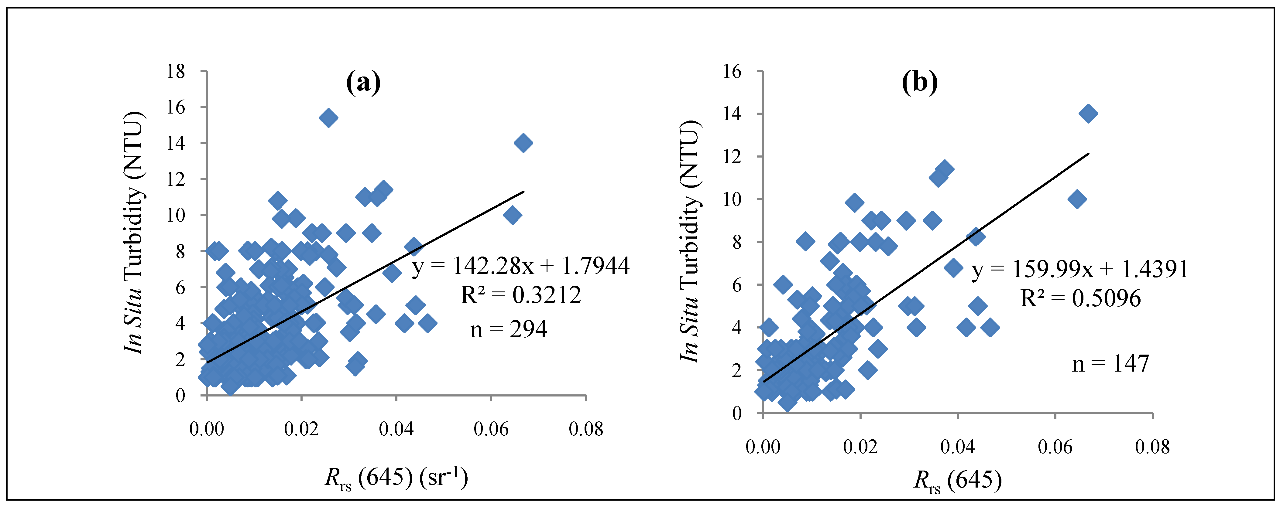
| 2.4 | 0.32 | 142.28 × Rrs + 1.79.44 | 294 |
| 1.4 | 0.23 | 131.33 × Rrs + 1.9265 | 394 |
| 0.4 | 0.20 | 116.53 × Rrs + 2.0798 | 414 |
2.3. Moderate Resolution Imaging Spectroradiometer (MODIS) Data
2.4. MODIS Data Processing
2.5. Variability of Empirical Relationships
2.6. Algorithm Development

3. Results and Discussion
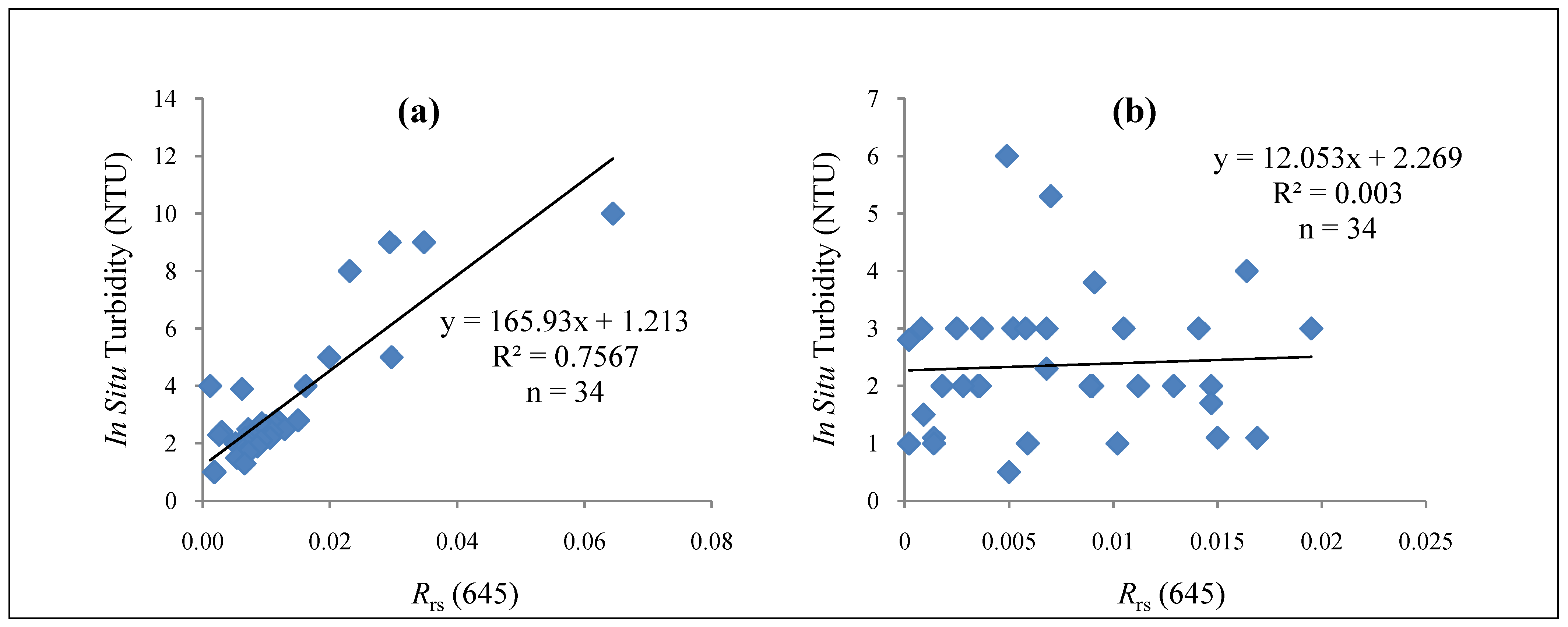
| Average | Average | ||||
|---|---|---|---|---|---|
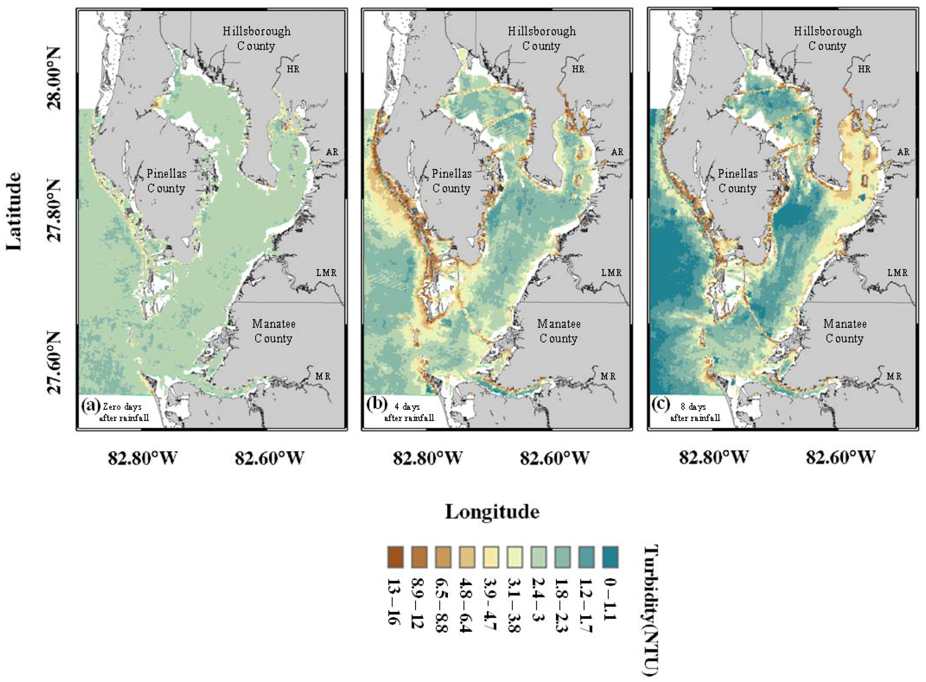
| Number of Days | Turbidity NTU | Turbidity NTU | R2 | Equation | n |
| 8 | 3.2 | 10 | 0.76 | 165.93 × Rrs + 1.213 | 34 |
| 7 | 3.7 | 8.2 | 0.60 | 142.86 × Rrs + 1.88 | 26 |
| 6 | 4.3 | 11 | 0.33 | 164.5 × Rrs + 1.9602 | 27 |
| 5 | 5.8 | 14 | 0.57 | 168.38 × Rrs + 3.7513 | 27 |
| 4 | 2.8 | 8 | 0.30 | 153.91 × Rrs + 1.3496 | 19 |
| 3 | 3.3 | 11 | 0.18 | 105.99 × Rrs + 1.7543 | 62 |
| 2 | 3.5 | 8 | 0.32 | 154.27 × Rrs + 1.5501 | 27 |
| 1 | 3.5 | 15.4 | 0.38 | 138.7 × Rrs + 1.6969 | 38 |
| 0 | 2.4 | 6 | 0.00 | 12.053 × Rrs + 2.269 | 34 |

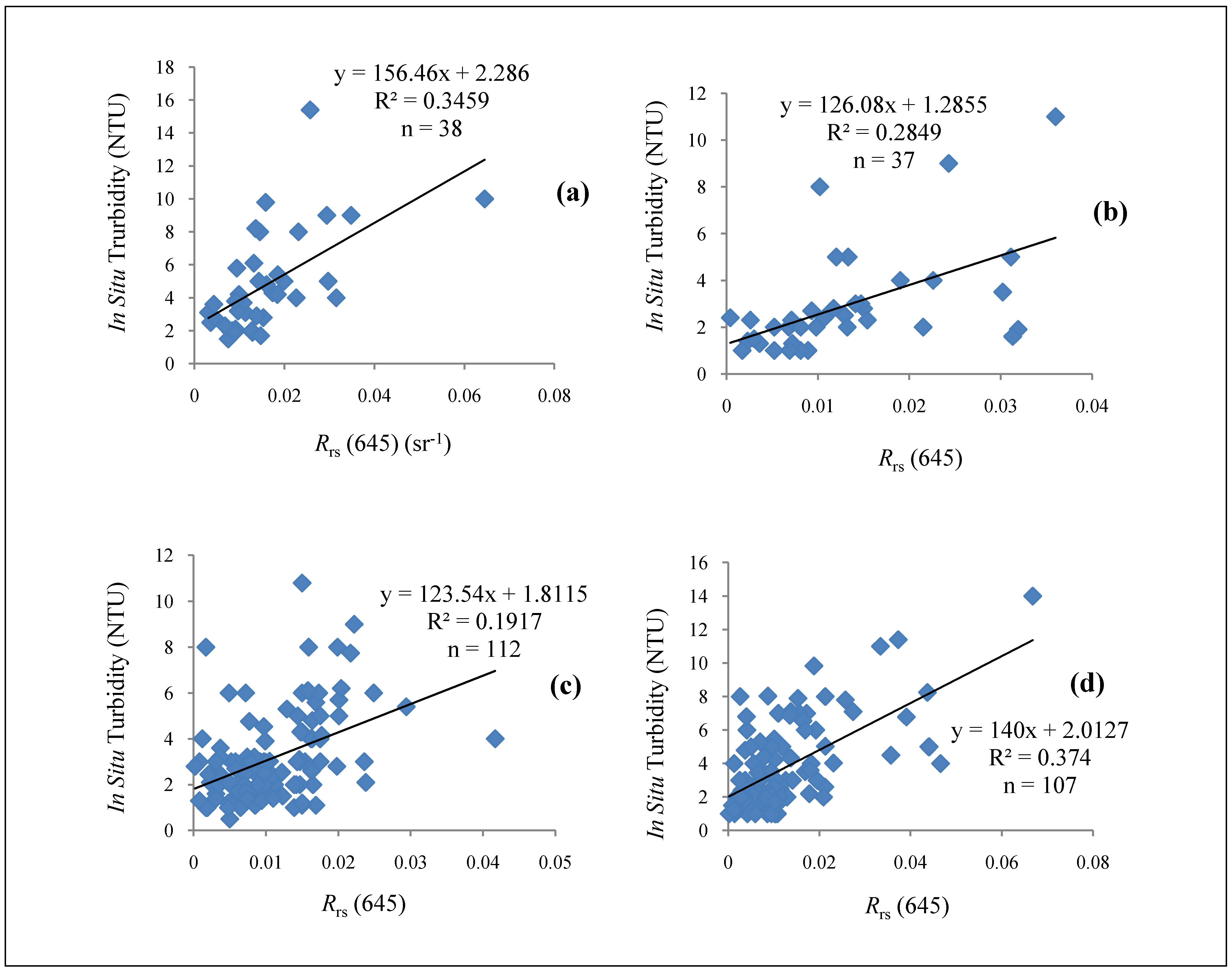
| Sub-Regions | Average Turbidity (NTU) | SD-Turbidity (NTU) | Average Bottom Depth (m) | SD-Bottom Depth (m) | Average Color (Pt-Co Units) | SD-Color (Pt-Co Units) | n |
|---|---|---|---|---|---|---|---|
| HB | 4.8 | 3.0 | 3.8 | 1.0 | 10.0 | 5.4 | 38 |
| OTB | 2.9 | 2.2 | 3.5 | 1.0 | 8.7 | 3.7 | 37 |
| MTB | 3.2 | 1.9 | 6.1 | 2.0 | 8.3 | 4.5 | 112 |
| LTB | 3.8 | 2.6 | 6.4 | 2.4 | 4.7 | 2.3 | 107 |

4. Conclusions
Acknowledgments
References
- Lee, S.; Ni-Meister, W. Monitoring coastal estuary water clarity using Landsat multispectral data. Middle States Geogr. 2006, 39, 43–51. [Google Scholar]
- Doxaran, D.; Froidefond, J.-M.; Castaing, P. Remote-sensing reflectance of turbid sediment-dominated water. Reduction of sediment type variations and changing illumination conditions effects by use of reflectance ratios. Appl. Opt. 2003, 42, 2623–2634. [Google Scholar] [CrossRef] [PubMed]
- Woodruff, D.L.; Stumff, R.O.; Scope, J.A. Remote estimation of water clarity in optically complex estuarine waters. Remote Sens. Environ. 1999, 68, 41–52. [Google Scholar] [CrossRef]
- Lahet, F.; Ouillon, S.; Forget, P. A Three-component model of ocean color and its application in the Ebro River mouth area. Remote Sens. Environ. 2000, 72, 181–190. [Google Scholar] [CrossRef]
- Moran, M.A. Distribution of terrestrially derived dissolved organic matter on the southeastern U. S. continental shelf. Limnol. Oceanogr. 1991, 36, 1134–1149. [Google Scholar] [CrossRef]
- Moran, M.A.; Hodson, R.H. Dissolved humic substances of vascular plant origin in a coastal marine environment. Limnol. Oceanogr. 1994, 39, 762–771. [Google Scholar] [CrossRef]
- Li, R.; Li, J. Satellite remote sensing technology for lake water clarity monitoring: An overview. Environ. Inf. Arch. 2004, 2, 893–901. [Google Scholar]
- Chen, Z.; Hu, C.; Muller-Karger, F. Monitoring turbidity in Tampa Bay using MODID/Aqua 250-m imagery. Remote Sens. Environ. 2007, 109, 207–220. [Google Scholar] [CrossRef]
- Rodríguez-Guzmán, V.; Gilbes-Santaella, F. Using MODIS 250 m imagery to estimate Total Suspended Sediment in a tropical open bay. Int. J. Syst. Appl. Eng. Devel. 2009, 3, 36–44. [Google Scholar]
- Doxaran, D.; Froidefond, J.-M.; Castaing, P.; Babin, M. Dynamics of the turbidity maximum zone in a macrotidal estuary (the Gironde, France): Observations from field and MODIS satellite data. Estuar. Coast. Shelf Sci. 2009, 81, 321–332. [Google Scholar] [CrossRef]
- Whitlock, C.H.; Poole, L.R.; Usry, J.W.; Houghton, W.M.; Witte, W.G.; Morris, W.D.; Gurganus, E.A. Comparison of reflectance with backscatter and absorption parameters for turbid waters. Appl. Opt. 1981, 20, 517–522. [Google Scholar] [CrossRef] [PubMed]
- Wong, M.S.; Nichol, J.E.; Lee, K.H.; Emerson, N. Modelling water quality using Terra/MODIS 500 m satellite images. In Proceedings of XXIst ISPRS Congress, Beijing, China, July 3–11, 2008; Volume XXXVII, pp. 679–684.
- National Oceanographic and Athmospheric Administration (NOAA). Tampa International Airport Station 2010. 9 April 2010. Available online: http://www.ncdc.noaa.gov/oa/mpp/index.html (accessed on August 19, 2010). [Google Scholar]
- Tampa Bay Estuary Program (TBEP). Charting the Course: The Comprehensive Conservation and Management Plan for Tampa Bay; TBEP: St. Petersburg, FL, USA, 2006. [Google Scholar]
- Lewis, R.R.; Whitman, R.L. A new geographic description of the boundaries and subdivisions of Tampa Bay, Florida. In Proceedings of the 1st Tampa Bay Area Scientific Information Symposium, Minneapolis, MN, USA, May 3–6, 1982; pp. 10–17.
- US Bureau of the Census. Annual Estimates of the Population of Metropolitan and Micropolitan Statistical Areas: April 1, 2000 to July 1, 2006; US Bureau of the Census: Washington, DC, USA, 2007. Available online: http://www.census.gov/popest/metro/CBSA-est2006-annual.html (accessed on September 2, 2010).
- Johansson, J.O.R. Historical overview of Tampa Bay water quality and seagrass: Issues and trends. In Proceedings of the Tampa Bay Estuary Program Symposium, St. Petersburg, FL, USA, August 22–24, 2000; pp. 1–10.
- Garrity, R.D.; McCann, N.; Murdoch, J. A review of the environmental impacts of municipal services in Tampa. In Proceedings of the 1st Tampa Bay Area Scientific Symposium (BASIS), Minneapolis, MN, USA, May 3–6, 1982.
- Water Atlas. 2010. Available online: http://www.wateratlas.usf.edu (accessed on August 19, 2010).
- Lehner, S.; Anders, I.; Gayer, G. High resolution of suspended particulate matter concentration in the German Bight. Earsel eProc. 2004, 3, 118–126. [Google Scholar]
- Stumpf, R.P; Pennock, J. Calibration of a general optical equation for remote sensing of suspended sediments in a moderately turbid estuary. J. Geophys. Res. 1989, 94, 14363–14371. [Google Scholar] [CrossRef]
- Koponen, S.; Pulliainen, J.; Kallio, K.; Vepsäläinen, J.; Hallikainen, M. Use of MODIS data for monitoring turbidity in Finnish Lakes. In Proceedings of the IEEE Geoscience and Remote Sensing Symposium (IGARSS’01), Sydney, Australia, July 9–13, 2001; pp. 2184–2186.
- Doxaran, D.; Froidefond, J.-M.; Lavander, S.; Castaing, P. Spectral signature of highly turbid waters appliocation with SPOT data to quantify suspended particulate matter concentrations. Remote Sens. Environ. 2002, 81, 149–161. [Google Scholar] [CrossRef]
- Vermote, E.F.; El Saleoql, N.; Justice, C.O.; Kaufman, Y.J.; Privette, J.L.; Remer, L.; Roger, J.C.; Tanré, D. Atmospheric correction of visible to middle-infrared EOS-MODIS data over land surfaces: background, operational algorithm and validation. J. Geophs. Res. 1997, 102, 17131–17141. [Google Scholar] [CrossRef]
- Doxaran, D.; Cherukuru, N.; Lavander, S. Surface reflection effects on upwelling radiance field measurements in turbid waters. J. Opt. A: Pure Appl. Opt. 2004, 6, 690–697. [Google Scholar] [CrossRef]
- US Geological Survey (USGS). Land Processes Distributed Active Archive Center (LP DAAC). 2010. Available online: https://lpdaac.usgs.gov/lpdaac/get_data/data_pool (accessed on January 4, 2010). [Google Scholar]
- Amin, A.R.M.; Abdullah, K. Discrimination of sediment and atmospheric contribution from turbid water for 0.66 μm channels. In Proceedings of the Map Asia 2010 & International Society for Gerontechnology 2010, Kuala Lumpur, Malaysia, July 26–28, 2010.
- D’Sa, E.J.; Hu, C.; Muller, F.E.; Carder, K.L. Estimation of colored dissolved organic matter and salinity fields in case 2 waters using Sea WiFS: Examples from Florida Bay and Florida Shelf. Indian Acad. Sci. Earth Planet Sci. 2002, 111, 197–207. [Google Scholar]
- Hu, C.; Carder, K.L.; Muller, F.E. Atmospheric Correction of SeaWiFS imagery over turbid coastal waters: A practical method. Remote Sens. Environ. 2001, 74, 195–206. [Google Scholar] [CrossRef]
- Fennessy, M.J.; Dyer, K.R.; Huntley, D.A. Size and settling velocity distributions of flocs in the Tamar estuary during a tidal cycle. Neth. J. Aquat. Ecol. 1994, 28, 275–282. [Google Scholar] [CrossRef]
- Eisma, D.; Li, A. Changes in suspended-matter floc size during the tidal cycle in the Dollar Estuary. Neth. J. Sea Res. 1993, 31, 107–117. [Google Scholar] [CrossRef]
- Schoellhamer, D.H. Sediemnt resuspension mechanisms in Old Tampa Bay, Florida. Estuar. Coast. Shelf Sci. 1995, 40, 603–620. [Google Scholar] [CrossRef]
- Eisma, D. Flocculation and de-flocculation of suspended matter in Estuaries. Neth. J. Sea Res. 1986, 20, 183–199. [Google Scholar] [CrossRef]
- Xian, G.; Crane, M. Assessments of urban growth in the Tampa Bay watershed using remote sensing data. Remote Sens. Environ. 2005, 97, 203–215. [Google Scholar] [CrossRef]
- Paerl, H.W. Coastal Eutrophication and Harmful Algal Blooms: Importance of Atmospheric Deposition and Groundwater as “New” Nitrogen and Other Nutrient Sources. Limnol Oceanogr 1997, 42, 1154–1165. [Google Scholar] [CrossRef]
- Peierls, B.L.; Paerl, H.W. Bioavailability of atmospheric organic nitrogen deposition to coastal phytoplankton. Limnol. Oceanogr. 1997, 42, 1819–1823. [Google Scholar] [CrossRef]
© 2010 by the authors; licensee MDPI, Basel, Switzerland. This article is an open access article distributed under the terms and conditions of the Creative Commons Attribution license (http://creativecommons.org/licenses/by/3.0/).
Share and Cite
Moreno-Madrinan, M.J.; Al-Hamdan, M.Z.; Rickman, D.L.; Muller-Karger, F.E. Using the Surface Reflectance MODIS Terra Product to Estimate Turbidity in Tampa Bay, Florida. Remote Sens. 2010, 2, 2713-2728. https://doi.org/10.3390/rs2122713
Moreno-Madrinan MJ, Al-Hamdan MZ, Rickman DL, Muller-Karger FE. Using the Surface Reflectance MODIS Terra Product to Estimate Turbidity in Tampa Bay, Florida. Remote Sensing. 2010; 2(12):2713-2728. https://doi.org/10.3390/rs2122713
Chicago/Turabian StyleMoreno-Madrinan, Max J., Mohammad Z. Al-Hamdan, Douglas L. Rickman, and Frank E. Muller-Karger. 2010. "Using the Surface Reflectance MODIS Terra Product to Estimate Turbidity in Tampa Bay, Florida" Remote Sensing 2, no. 12: 2713-2728. https://doi.org/10.3390/rs2122713
APA StyleMoreno-Madrinan, M. J., Al-Hamdan, M. Z., Rickman, D. L., & Muller-Karger, F. E. (2010). Using the Surface Reflectance MODIS Terra Product to Estimate Turbidity in Tampa Bay, Florida. Remote Sensing, 2(12), 2713-2728. https://doi.org/10.3390/rs2122713