Application of Vegetation Indices for Agricultural Crop Yield Prediction Using Neural Network Techniques

Abstract
:1. Introduction
2. Methods, and Materials
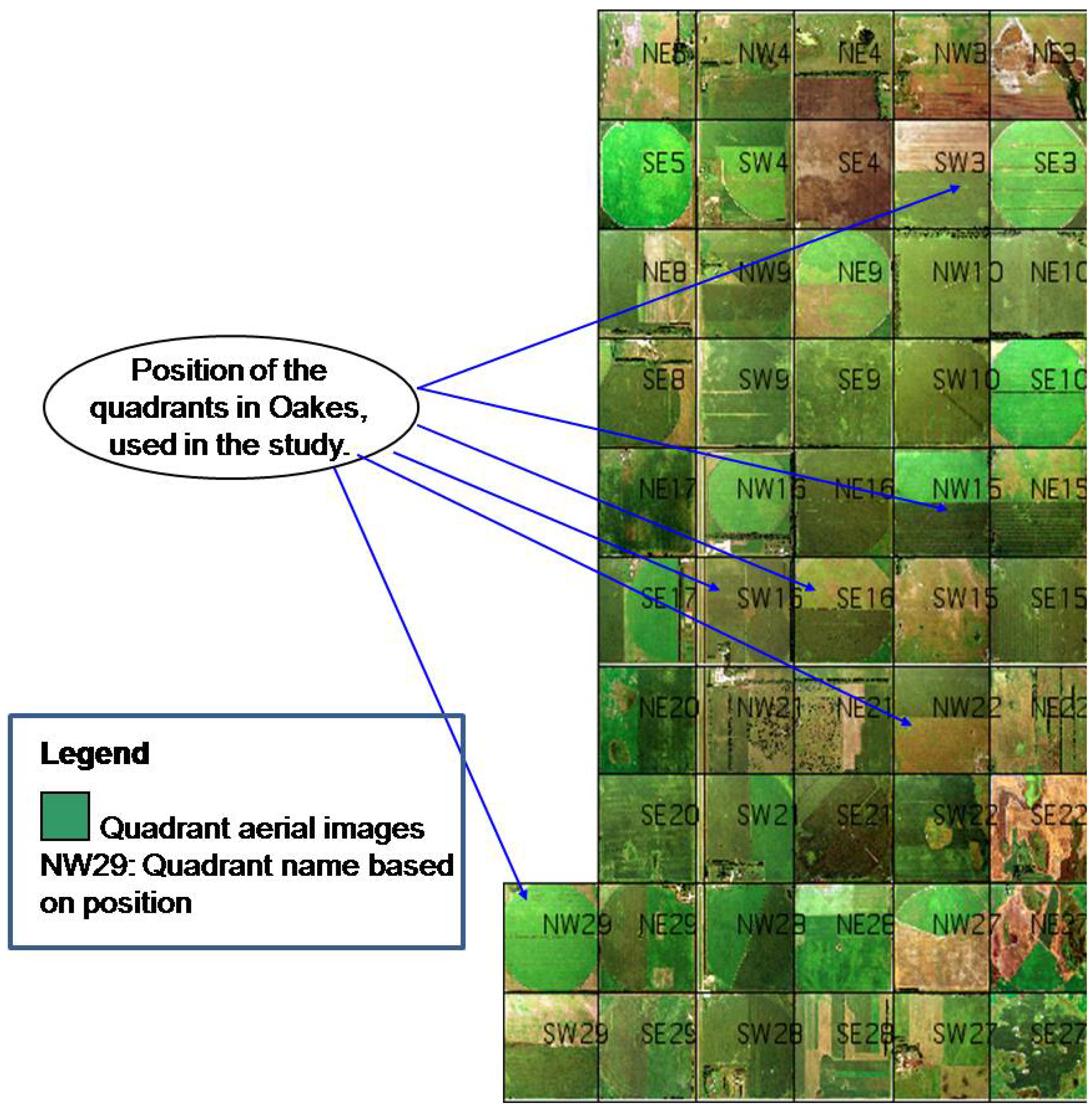
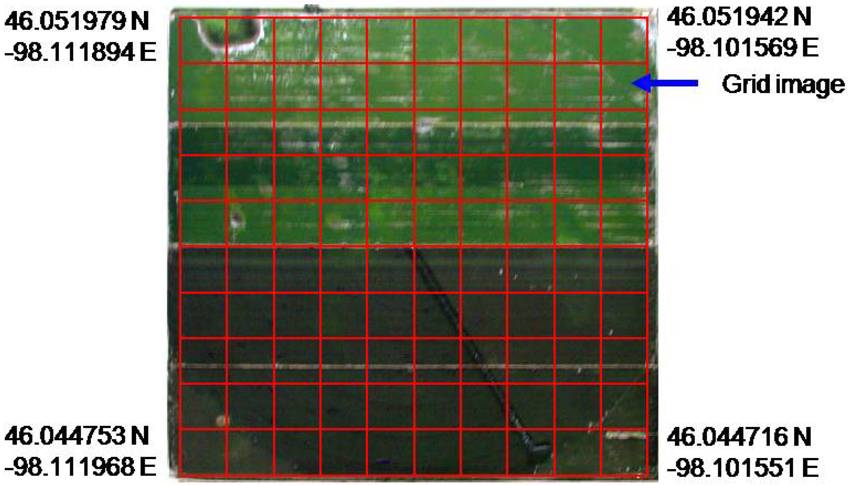
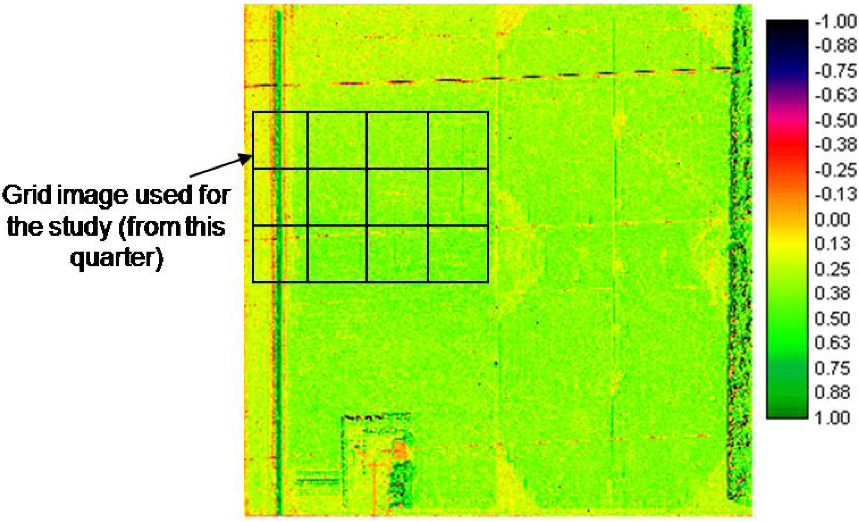
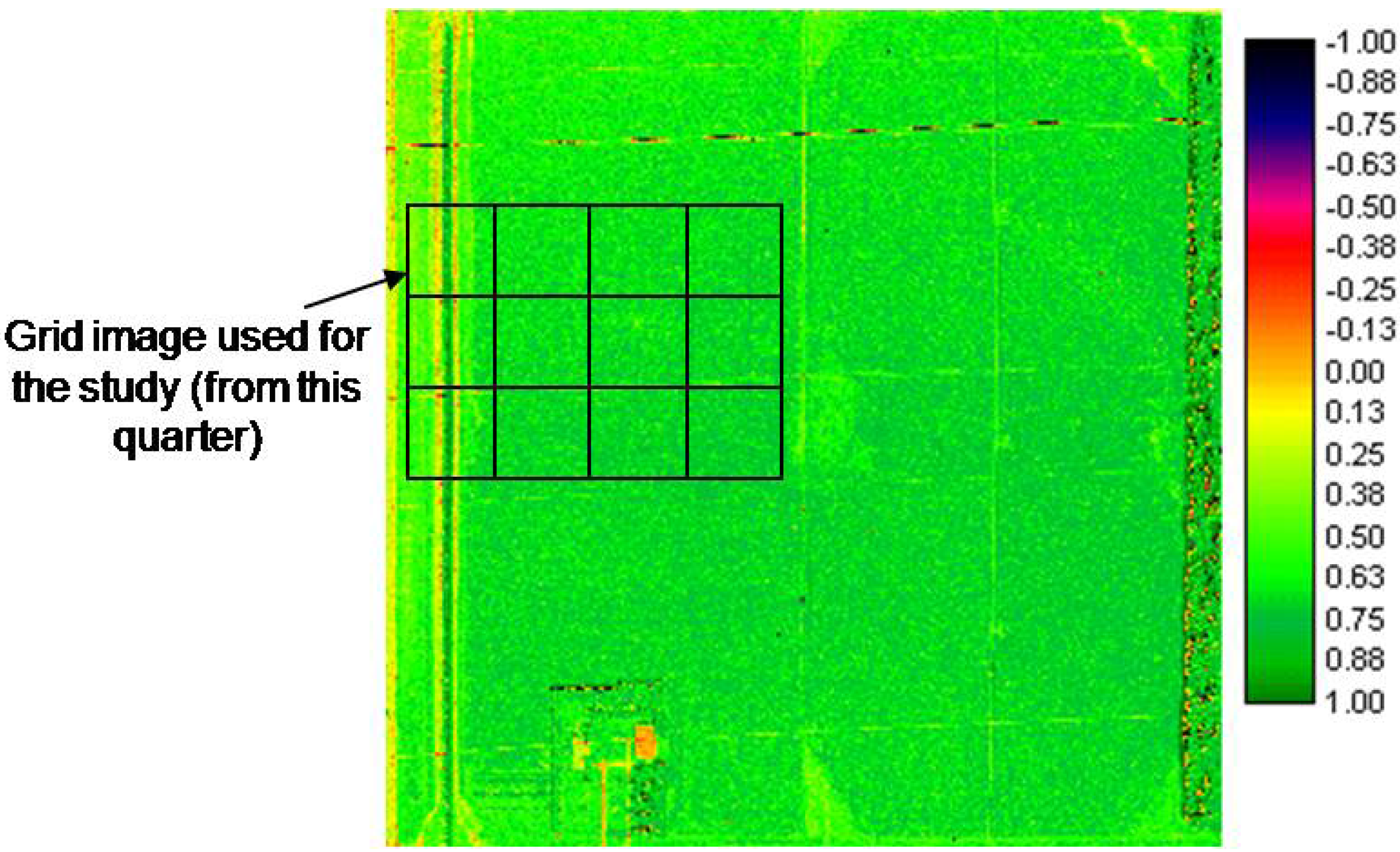
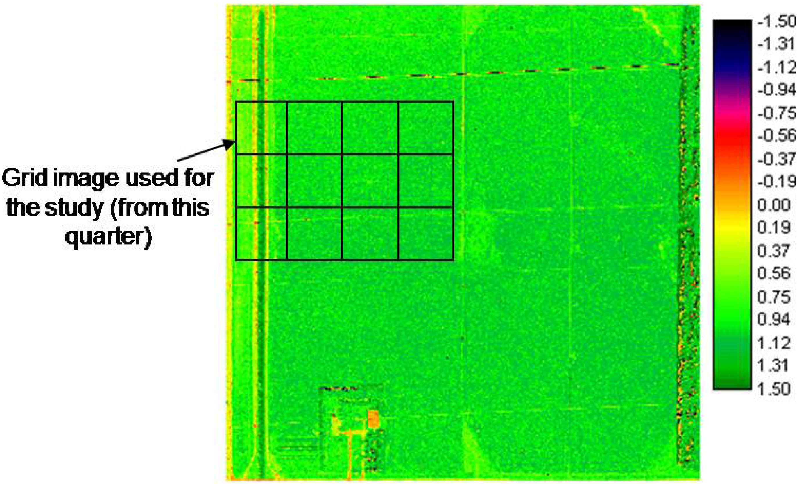
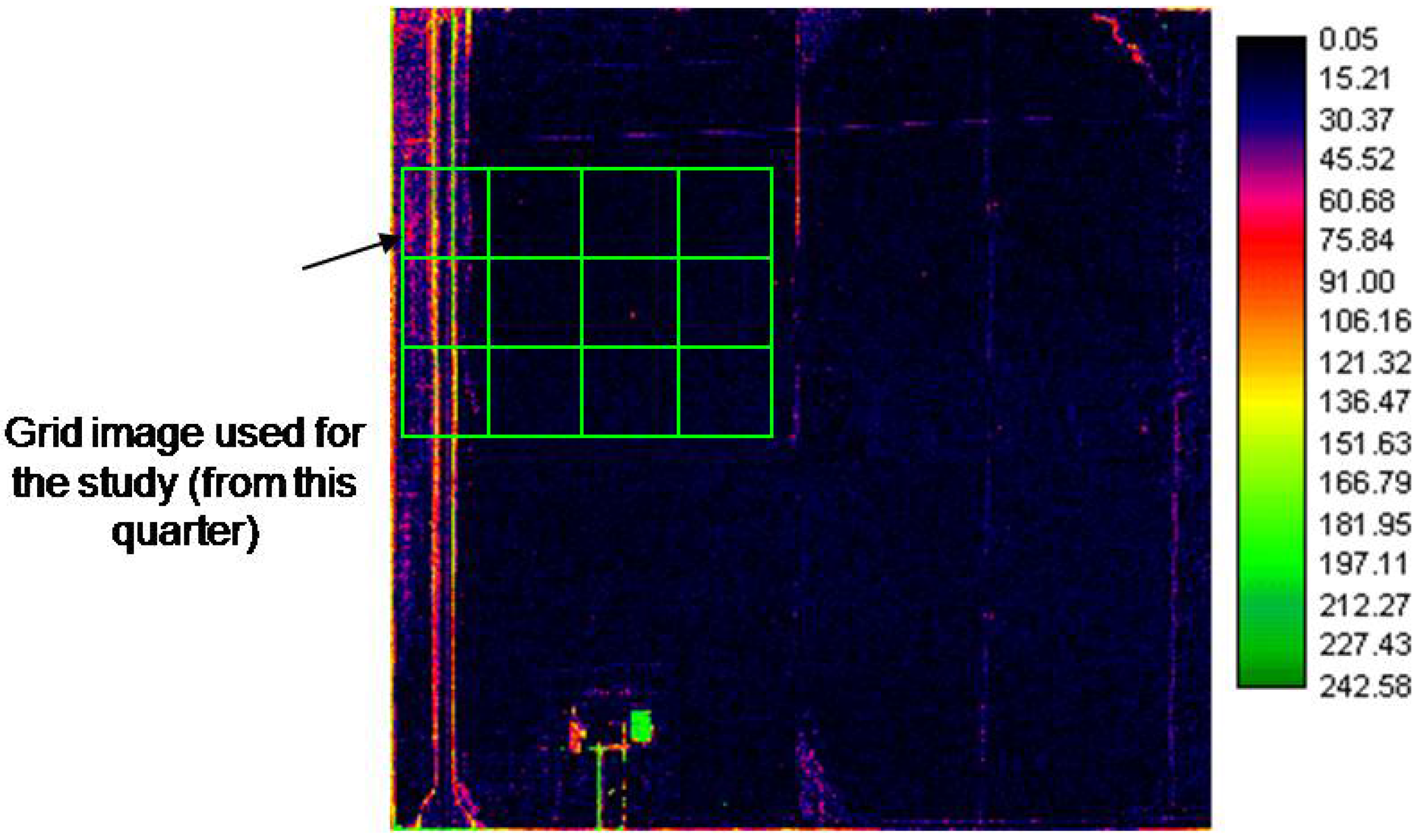
2.1. Study Area and Aerial Images Acquisition


| Year | Training data | Testing data | Remarks | ||
| Number of observations | Data from quadrants | Number of observations | Data from quadrants | ||
| 1998 | 100 | 29NW* | 31 | 16SW, 03SW, and 15NW | Training and test quarters are totally different |
| 1999 | 80 | 15NW, SW03 and 22NW | 21 | 16SW and 16SE | Training and test data generated by random selection from a combination of various quadrants |
| 2001 | 100 | 22NW | 30 | 29NW | Model trained and tested on individual quarter information |
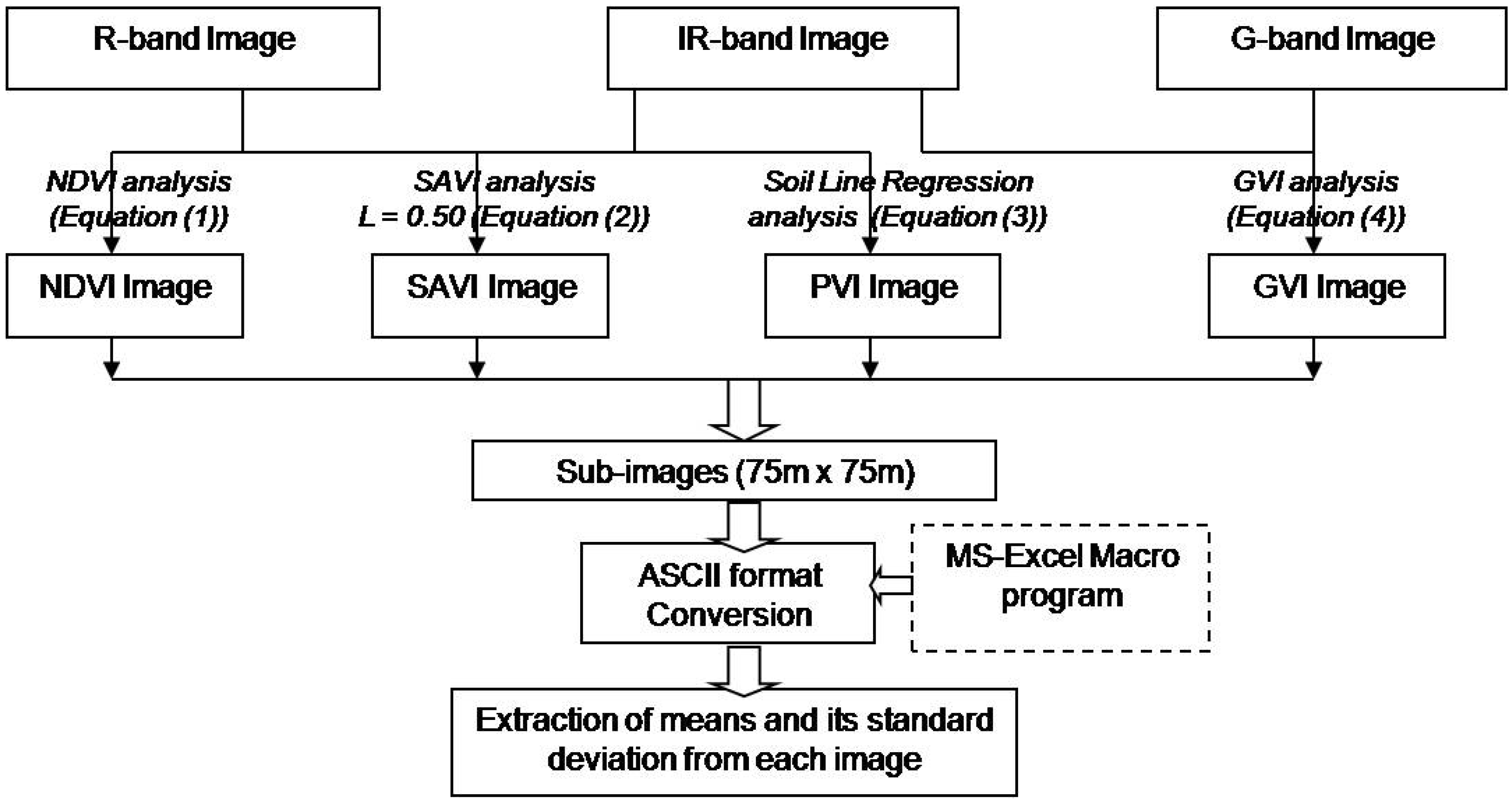
2.2. Extraction of Vegetation Indices


2.3. Yield Data Collection
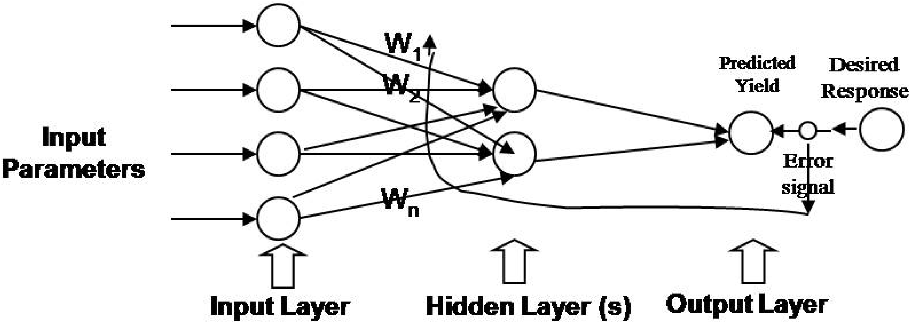
2.4. Neural Network Development
2.4.1. Input-output architecture of the NN model
2.4.2. Data preprocessing/mining of input parameters
2.4.3. Processing of output parameters
| Optimized net architecture and network parameters | Testing prediction accuracy (%) | Actual-Predicted output linear-fit parameters | ||||||||||||||||||
|---|---|---|---|---|---|---|---|---|---|---|---|---|---|---|---|---|---|---|---|---|
| Net arch.f | μa | ηb | epochs | Max. | Min. | Avg. | ac | βd | r-sqe | SEP (t/ha) | ||||||||||
| GVI 98 | 2-1-1 | 0.1 | 0.1 | 5,000 | 57.58 | 9.69 | 24.26 | 136.1 | 0.72 | 0.49 | 1.65 | |||||||||
| NDVI 98 | 2-1-1 | 0.1 | 0.1 | 5,000 | 42.10 | 10.76 | 19.36 | 128.4 | 1.23 | 0.16 | 1.98 | |||||||||
| PVI 98 | 2-1-1 | 0.1 | 0.1 | 5,000 | 99.38 | 25.81 | 83.50 | 68.5 | 0.56 | 0.69 | 1.82 | |||||||||
| SAVI 98 | 2-1-1 | 0.1 | 0.1 | 5,000 | 41.87 | 10.67 | 19.24 | 128.7 | 1.23 | 0.16 | 1.98 | |||||||||
| GVI 99 | 2-1-1 | 0.1 | 0.5 | 5,000 | 99.99 | 66.77 | 93.86 | −326.4 | 2.76 | 0.53 | 0.68 | |||||||||
| NDVI 99 | 2-1-1 | 0.1 | 0.1 | 5,000 | 99.74 | 70.14 | 91.36 | −111.4 | 1.59 | 0.38 | 0.62 | |||||||||
| PVI 99 | 2-1-1 | 0.1 | 0.1 | 5,000 | 99.35 | 64.49 | 93.03 | −186.8 | 1.98 | 0.25 | 0.75 | |||||||||
| SAVI 99 | 2-1-1 | 0.1 | 0.1 | 5,000 | 99.68 | 70.20 | 95.37 | −105.6 | 1.56 | 0.53 | 0.61 | |||||||||
| GVI 01 | 2-1-1 | 0.1 | 0.9 | 10,000 | 99.78 | 77.61 | 94.85 | −1520.9 | 9.14 | 0.30 | 0.61 | |||||||||
| NDVI 01 | 2-1-1 | 0.5 | 0.5 | 50,000 | 99.79 | 81.53 | 95.04 | 693.7 | −2.82 | 0.22 | 0.68 | |||||||||
| PVI 01 | 2-1-1 | 0.1 | 0.1 | 50,000 | 99.97 | 79.34 | 96.04 | −64.8 | 1.35 | 0.09 | 0.60 | |||||||||
| SAVI 01 | 2-1-1 | 0.5 | 0.5 | 50,000 | 99.79 | 81.54 | 95.04 | 690.5 | −2.80 | −0.22 | 0.68 | |||||||||
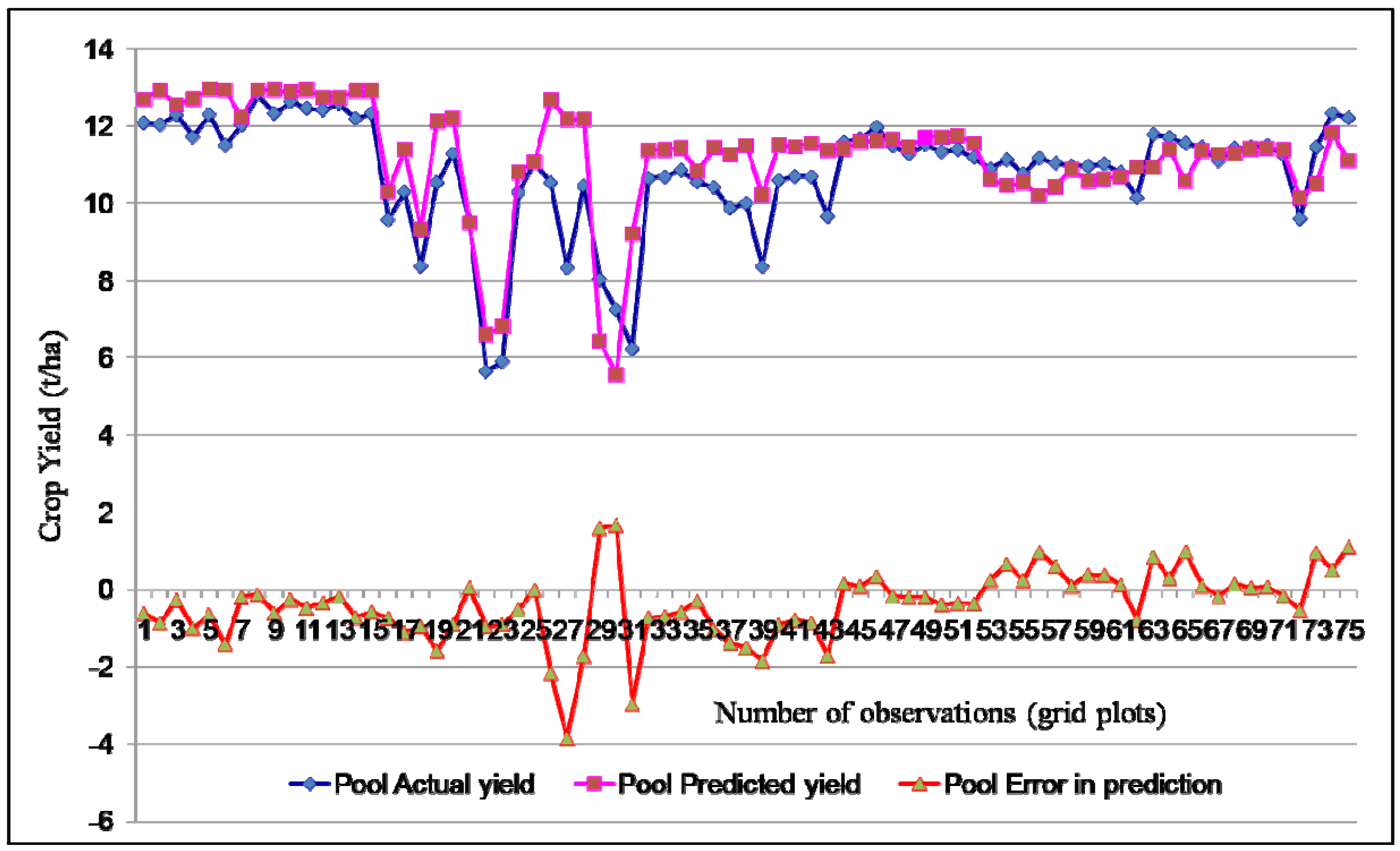
| GVI (Pool)h | 2-1-1 | 0.1 | 0.5 | 5,000 | 99.55 | 69.63 | 91.81 | −23.9 | 5.25 | 0.37 | 0.80 | |||||||||
| NDVI (Pool) | 2-1-1 | 0.5 | 0.5 | 10,000 | 98.44 | 77.54 | 89.11 | 245.6 | −4.77 | 0.31 | 0.77 | |||||||||
| PVI (Pool) | 2-1-1 | 0.1 | 0.9 | 5,000 | 99.87 | 79.58 | 94.27 | −54.8 | 0.95 | 0.45 | 0.55 | |||||||||
| SAVI (Pool) | 2-1-1 | 0.1 | 0.1 | 50,000 | 98.59 | 71.34 | 92.11 | 350.8 | −2.80 | 0.32 | 0.64 | |||||||||
2.4.4. Neural network model development and evaluation

3. Results and Discussion
3.1. Best Date Image Selection for the Study
3.2. VI image Analyses and Soil Line Information for PVI Analysis


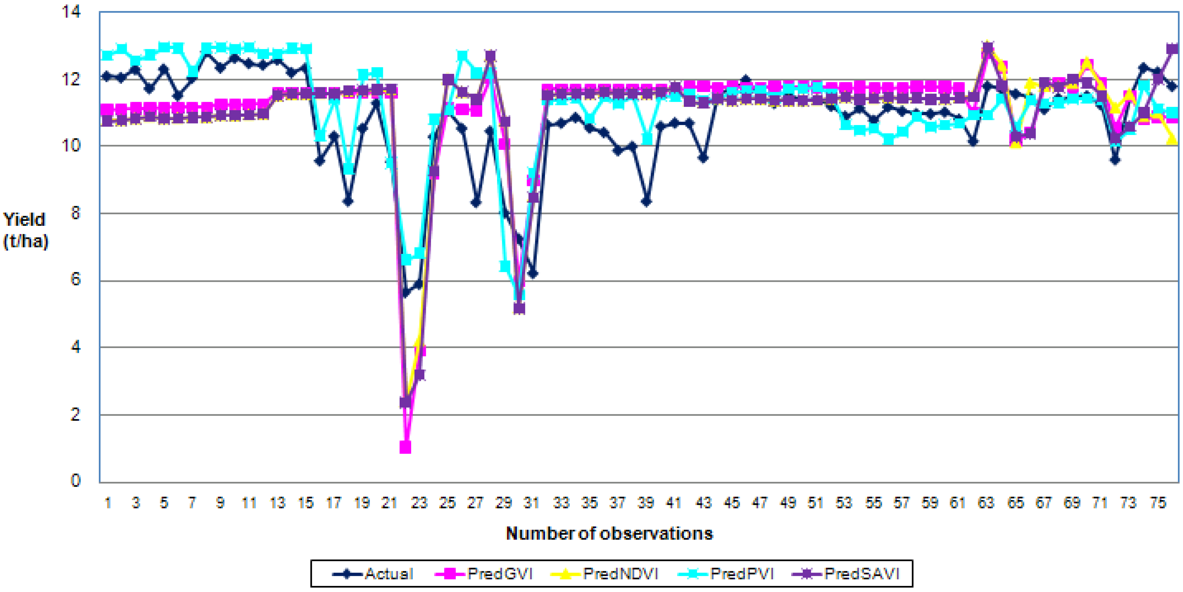
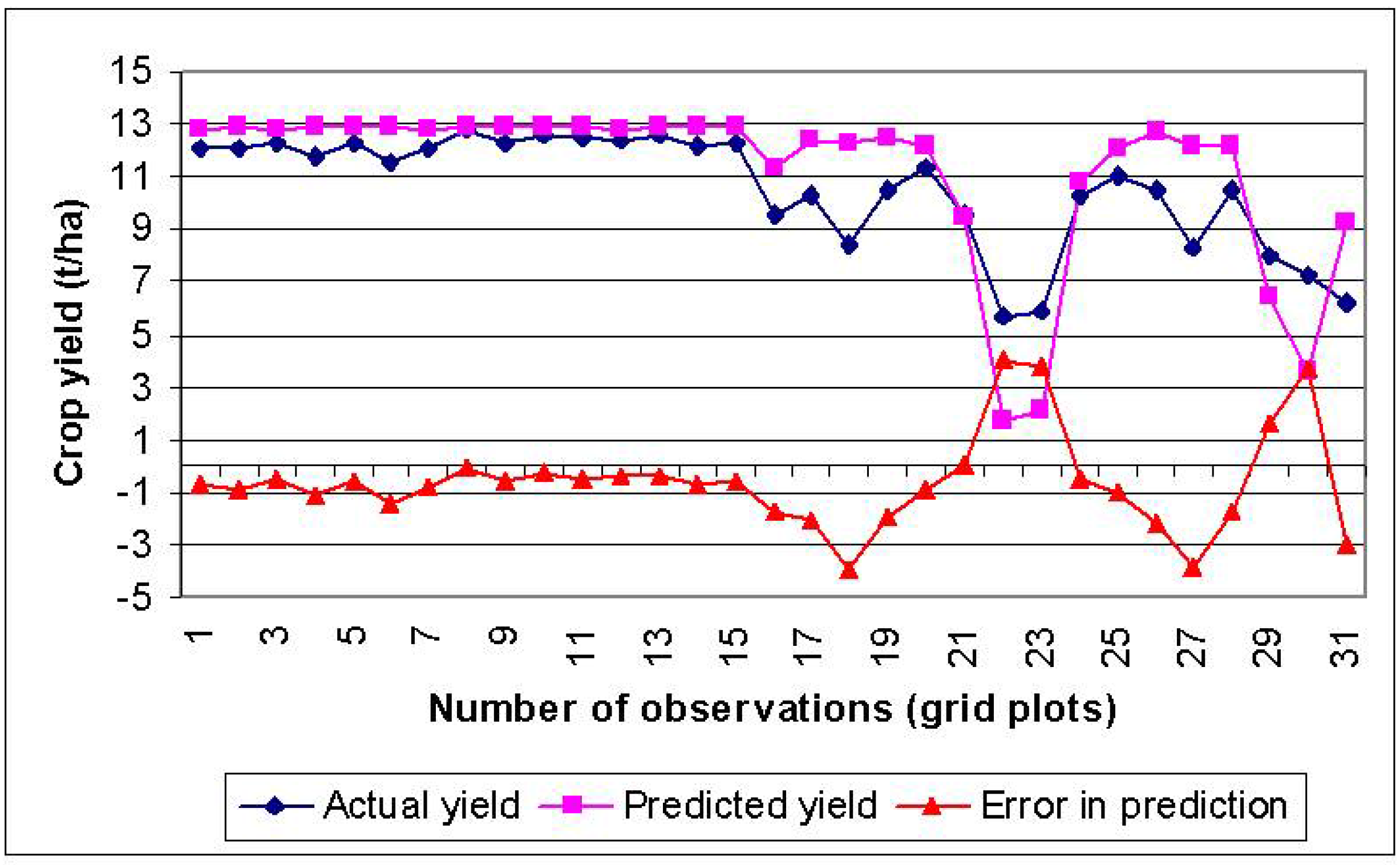
3.3. Performance Evaluation of VI-BPNN Models
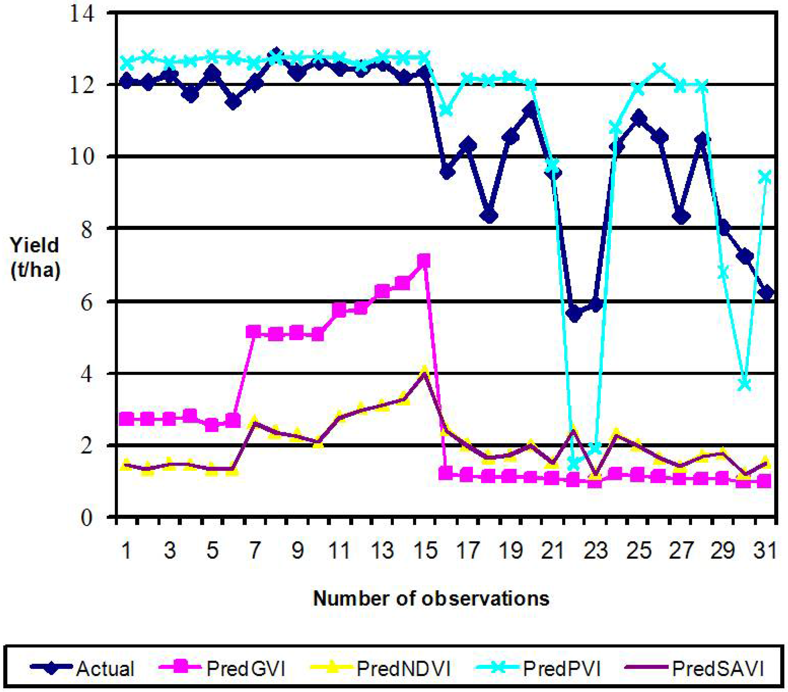
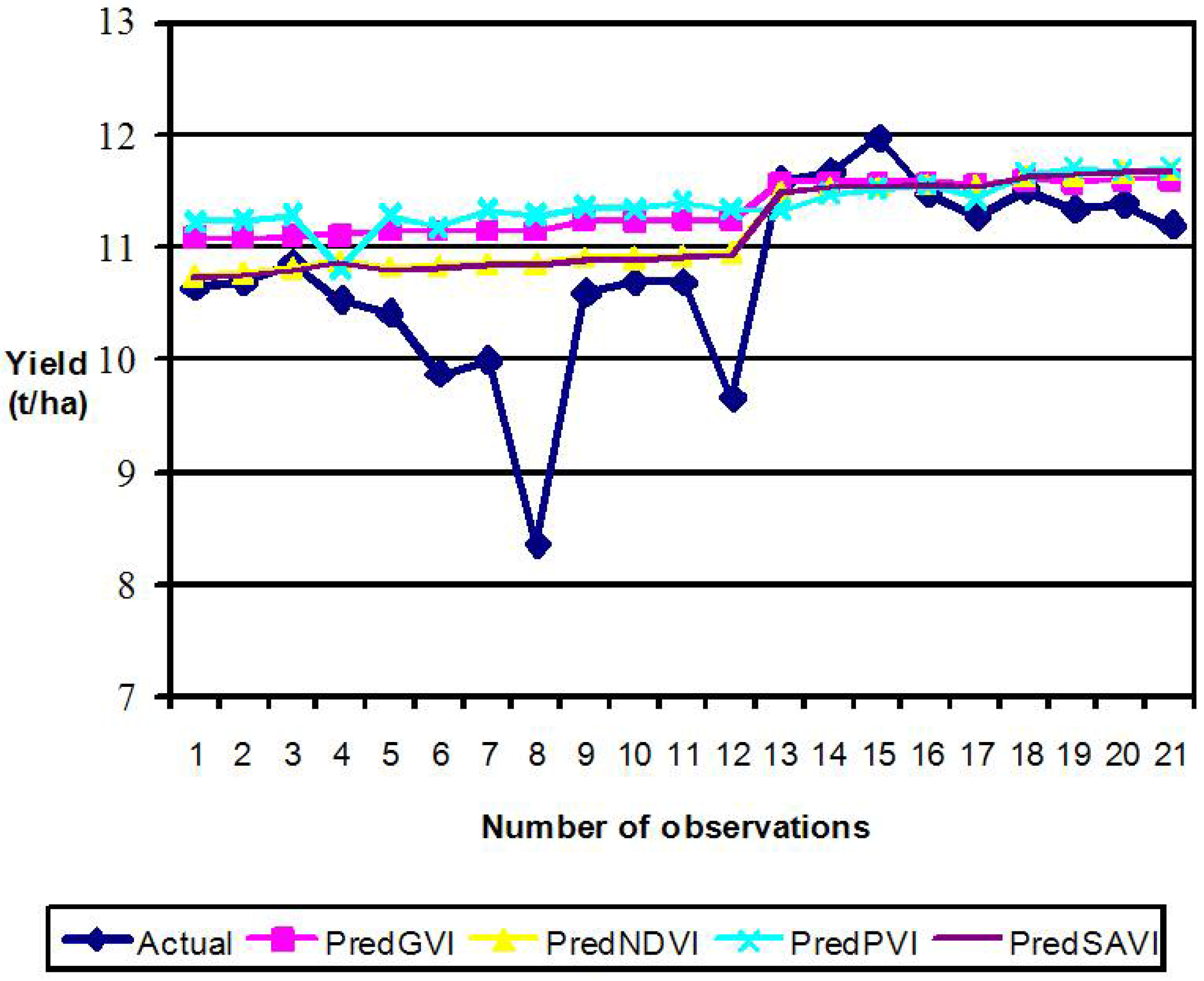
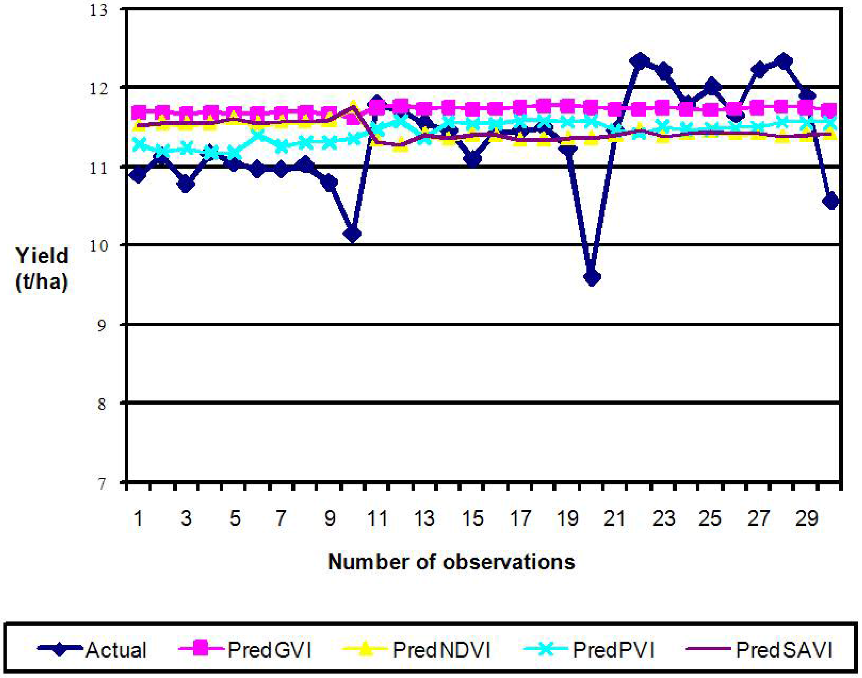
3.4. Individual VI Models


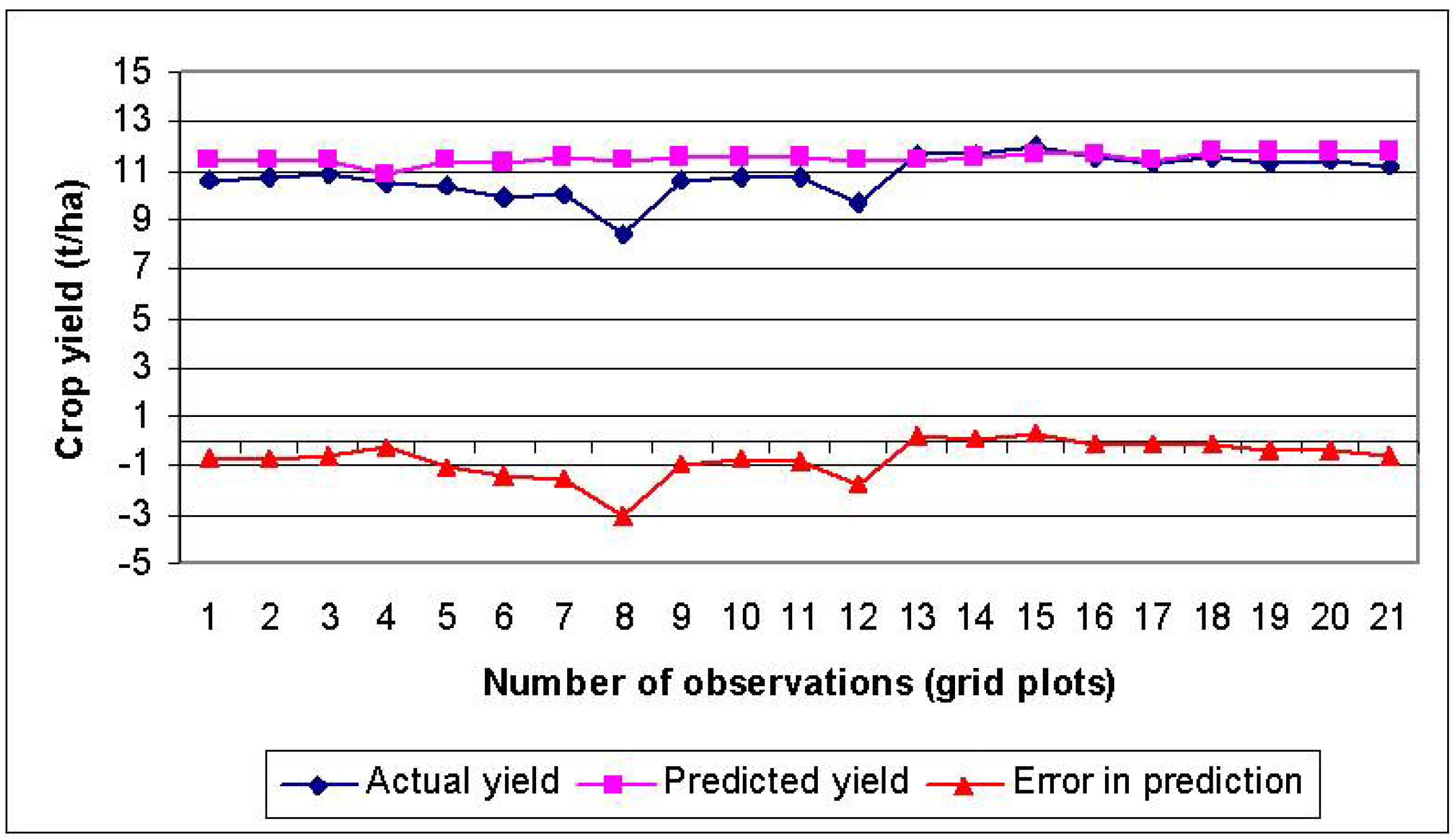
3.5. Performance Evaluation of Neural Networks with log10-Transformed Datasets (PVI)
3.6. Transformed BPNN PVI Models
| Model | Optimal Net | Testing Models | Testing Results | |||||||
| Optimal model parameters | Linear fit equation | Accuracy (%) | ||||||||
| Learning rate | Momentum term | r-sqa | ab | βc | SEPd (t/ha) | Min. | Max. | Avg. | ||
| Transformede PVI 98 | 2-1-1 | 0.1 | 0.1 | 0.69 | 0.64 | 0.37 | 0.15 | 29.78 | 99.75 | 90.00 |
| Transformed PVI 99 | 2-1-1 | 0.1 | 0.1 | 0.20 | −1.0 | 1.94 | 0.03 | 85.44 | 99.90 | 96.91 |
| Transformed PVI 01 | 2-1-1 | 0.1 | 0.1 | 0.21 | 0.79 | 0.26 | 0.03 | 92.24 | 99.83 | 97.79 |
| Transformed PVI (Pool)f | 2-1-1 | 0.1 | 0.9 | 0.72 | 0.55 | 0.35 | 0.05 | 69.78 | 98.97 | 93.05 |


4. Conclusions
Acknowledgment
References and Notes
- Taylor, J.C.; Wood, G.A.; Thomas, G. Mapping yield potential with remote sensing. Precis. Agric. 1997, 1, 713–720. [Google Scholar]
- Magri, A. Soil test, aerial image and yield data as inputs for site-specific fertility and hybrid management under maize. Precis. Agric. 2005, 6, 87–110. [Google Scholar] [CrossRef]
- Baez-Gonzalez, A.D.; Kiniry, J.R.; Maas, S.J.; Tiscareno, M.L.; Macias, J.C.; Mendoza, J.L.; Richardson, C.W.; Salinas, J.G.; Manjarrez, J.R. Large-area maize yield forecasting using leaf area index based yield model. Agron. J. 2005, 97, 418–425. [Google Scholar] [CrossRef]
- Lobell, D.B.; Ortiz-Monasterio, J.I.; Asner, G.P.; Naylor, R.L.; Falcon, W.P. Combining field surveys, remote sensing, and regression trees to understand yield variations in an irrigated wheat landscape. Agron. J. 2005, 97, 241–249. [Google Scholar]
- Yang, P.; Tan, G.X.; Zha, Y.; Shibasaki, R. Integrating remotely sensed data with an ecosystem model to estimate crop yield in north China. In Proceedings of XXth ISPRS Congress Proceedings Commission VII, WG VII/2, Istanbul, Turkey, 2004; pp. 150–156.
- Doraiswamy, P.C.; Moulin, S.; Cook, P.W.; Stern, A. Crop yield assessment from remote sensing. Photogramm. Eng. Remote Sens. 2003, 69, 665–674. [Google Scholar] [CrossRef]
- Tan, G.; Shibasaki, R. Global estimation of crop productivity and the impacts of global warming by GIS and EPIC integration. Ecol. Model. 2003, 168, 357–370. [Google Scholar] [CrossRef]
- Baez-Gonzalez, A.D.; Chen, P.; Tiscareno-Lopez, M.; Srinivasan, R. Using satellite and field data with crop growth modeling to monitor and estimate corn yield in Mexico. Crop Science 2002, 42, 1943–1949. [Google Scholar] [CrossRef]
- Plant, R.E.; Munk, D.S.; Roberts, B.R.; Vargas, R.L.; Rains, D.W.; Travis, R.L.; Hutmacher, R.B. Relationship between remotely sensed reflectance data and cotton growth and yield. Trans. ASAE 2000, 43, 535–546. [Google Scholar] [CrossRef]
- Sun, J. Dynamic monitoring and yield estimation of crops by mainly using the remote sensing technique in China. Photogramm. Eng. Remote Sens. 2000, 66, 645–650. [Google Scholar]
- Lillesand, T.M.; Keifer, R.W. Remote Sensing and Image Interpretation, 3rd ed.; John Willey and Sons: New York, NY, USA, 1994; p. 750. [Google Scholar]
- GopalaPillai, S.; Tian, L. In-field variability detection and yield prediction in corn using digital aerial imaging. Trans. ASAE 1999, 42, 1911–1920. [Google Scholar] [CrossRef]
- Senay, G.B.; Ward, A.D.; Lyon, J.G.; Fausey, N.R.; Nokes, S.E. Manipulation of high spatial resolution aircraft remote sensing data for use in site specific farming. Trans. ASAE 1998, 41, 489–495. [Google Scholar] [CrossRef]
- Thiam, S. Chapter on vegetation indices. In Guide to GIS and Image Processing; Volume 2; Idrisi Production: Clarke University, Worcester, MA, USA, 1999; pp. 107–122. [Google Scholar]
- Yang, C.; Anderson, G.L. Mapping grain sorghum yield variability using airborne digital videography. Precis. Agric. 2000, 2, 7–23. [Google Scholar] [CrossRef]
- Funk, C.; Budde, M. Phenologically-tuned MODIS NDVI-based production anomaly estimates for Zimbabwe. Remote Sens. Environ. 2009, 113, 115–125. [Google Scholar] [CrossRef]
- Rouse, J.W.; Haas, R.H.; Schell, J.A.; Deering, D.W. Monitoring vegetation systems in the Great Plains with ERTS. In Proceedings of Third ERTS Symposium, Greenbelt, MD, December 1974; NASA SP-351-1. pp. 309–317.
- Kriegler, F.J.; Malila, W.A.; Nalepka, R.F.; Richardson, W. Preprocessing transformations and their effects on multi-spectral recognition. In Proceedings of the Sixth International Symposium on Remote Sensing of Environment, University of Michigan, Ann Arbor, MI, USA, 1969; pp. 97–131.
- Lecain, D.R.; Morgan, J.A.; Schuman, G.E.; Reeder, J.D.; Hart, R.H. Carbon exchange rates in grazed and ungrazed pastures of Wyoming. J. Range Manage. 2000, 53, 199–206. [Google Scholar] [CrossRef]
- Todd, S.W.; Hoffer, R.M. Responses of spectral indices to variations in vegetation cover and soil background. Photogramm. Eng. Remote Sens. 1998, 64, 915–921. [Google Scholar]
- Bouman, B.A.M. Crop modeling and remote sensing for yield prediction. J. Agr. Sci. 1995, 43, 143–161. [Google Scholar]
- Huete, A.R.; Jackson, R.D. Soil and atmosphere influences on the spectra of partial canopies. Remote Sens. Environ. 1988, 25, 89–105. [Google Scholar] [CrossRef]
- Miura, T.; Huete, A.R.; Yoshioka, H. Evaluation of sensor calibration uncertainties on vegetation indices for MODIS. IEEE Trans. Geosci. Remote Sens. 2000, 38, 1399–1409. [Google Scholar] [CrossRef]
- Jayaraman, V.; Srivastava, S.K.; Raju, D.K.; Rao, U.R. Total solution approach using IRS-1C and IRS-P3 data. IEEE Trans. Geosci. Remote Sens. 2000, 38, 587–604. [Google Scholar] [CrossRef]
- Lamb, D.W.; Weedon, M.M.; Rew, L.J. Evaluating the accuracy of mapping weeds in seedling crops using airborne digital imaging: Avena spp. in seedling triticale. Weed Res. 1999, 39, 481–492. [Google Scholar] [CrossRef]
- Huete, A.R. A soil adjusted vegetation index (SAVI). Remote Sens. Environ. 1988, 25, 295–309. [Google Scholar] [CrossRef]
- Casanova, D.; Epema, G.F.; Goudriaan, J. Monitoring rice reflectance at field level for estimating biomass and LAI. Field Crop Res. 1998, 55, 83–92. [Google Scholar] [CrossRef]
- Elvidge, C.D.; Chen, Z.K. Comparison of broad-band and narrow-band red and near-infrared vegetation indices. Remote Sens. Environ. 1995, 54, 38–48. [Google Scholar] [CrossRef]
- Borge, N.H.; Leblanc, E. Comparing prediction power and stability of broadband and hyper spectral vegetation indices for estimation of green leaf area index and canopy chlorophyll density. Remote Sens. Environ. 2001, 76, 156–172. [Google Scholar] [CrossRef]
- Saltz, D.; Schmidt, H.; Rowen, M.; Karnieli, A.; Ward, D. Assessing grazing impacts by remote sensing in hyper-arid environments. J. Range Manage. 1999, 52, 500–507. [Google Scholar] [CrossRef]
- Mandal, U.K.; Victor, U.S.; Srivastava, N.N.; Sharma, K.L.; Ramesh, V.; Vanaja, M.; Korwar, G.R.; Ramakrishna, Y.S. Estimating yield of Sorghum using root zone water balance model and spectral characteristics of crop in dryland Alfisol. Agr. Water Manage. 2007, 87, 315–327. [Google Scholar] [CrossRef]
- Black, C.A. Soil Fertility Evaluation and Control; CRC Press: Boca Raton, FL, USA, 1993; pp. 92–103. [Google Scholar]
- Haykin, S. Neural Networks A Comprehensive Foundation, 2nd ed.; Prentice Hall Inc.: Upper Saddle River, NJ, USA, 1999; pp. 156–255. [Google Scholar]
- Lacroix, R.; Salehi, F.; Yang, X.Z.; Wade, K.M. Effects of data preprocessing on the performance of artificial neural networks for diary yield prediction and cow culling classification. Trans. ASAE 1997, 40, 839–846. [Google Scholar] [CrossRef]
- Zhuang, X.; Engel, B. Classification of multi-spectral remote sensing data using neural network vs. statistical methods. In ASAE Paper No. 90-7552; St. Joseph, MI, USA, 1990. [Google Scholar]
- Ranaweera, D.K.; Hubele, N.F.; Papalexopoulos, A.D. Application of radial basis function neural network model for short-term load forecasting. IEEE Proc.-Gener. Transm. Distrib. 1995, 142, 45–50. [Google Scholar] [CrossRef]
- Moshou, D.; Ramon, H.; Baerdemaeker, J.D. A weed species spectral detector based on neural networks. Precis. Agric. 2002, 3, 209–223. [Google Scholar] [CrossRef]
- Richardson, A.J.; Weigand, C.L. Distinguishing vegetation from background information. Photogramm.Eng. Remote Sens. 1977, 43, 1541–1552. [Google Scholar]
- Han, J.; Kamber, M. Data Mining: Concepts and Techniques; Morgan Kaufmann Publishers: San Francisco, CA, USA, 2001; p. 550. [Google Scholar]
- Sarle, W.S. Available online: ftp://ftp.sas.com/pub/neural/FAQ3.html (accessed on 15 July 2009).
- Jhang, Q.; Panigrahi, S.; Panda, S.S.; Borhan, M.S. Techniques for yield prediction from corn aerial images—a neural network approaching. Agr. Biosyst. Eng. 2002, 3, 18–28. [Google Scholar]
- Kramer, R. Chemometric Technique for Quantitative Analysis; Marcel Dekker Inc.: New York, NY, USA, 1998; pp. 120–121. [Google Scholar]
- Panda, S.S. Data mining Application in Production Management of Crop (Paper 1) . Ph.D. Dissertation, North Dakota State University, Fargo, ND, USA, 2002. [Google Scholar]
- Neural Ware. Reference Guide of Neural Ware; Neural Ware: Carnegie, PA, USA, 2008. [Google Scholar]
© 2010 by the authors; licensee Molecular Diversity Preservation International, Basel, Switzerland. This article is an open-access article distributed under the terms and conditions of the Creative Commons Attribution license (http://creativecommons.org/licenses/by/3.0/).
Share and Cite
Panda, S.S.; Ames, D.P.; Panigrahi, S. Application of Vegetation Indices for Agricultural Crop Yield Prediction Using Neural Network Techniques. Remote Sens. 2010, 2, 673-696. https://doi.org/10.3390/rs2030673
Panda SS, Ames DP, Panigrahi S. Application of Vegetation Indices for Agricultural Crop Yield Prediction Using Neural Network Techniques. Remote Sensing. 2010; 2(3):673-696. https://doi.org/10.3390/rs2030673
Chicago/Turabian StylePanda, Sudhanshu Sekhar, Daniel P. Ames, and Suranjan Panigrahi. 2010. "Application of Vegetation Indices for Agricultural Crop Yield Prediction Using Neural Network Techniques" Remote Sensing 2, no. 3: 673-696. https://doi.org/10.3390/rs2030673
APA StylePanda, S. S., Ames, D. P., & Panigrahi, S. (2010). Application of Vegetation Indices for Agricultural Crop Yield Prediction Using Neural Network Techniques. Remote Sensing, 2(3), 673-696. https://doi.org/10.3390/rs2030673