Forecasting Areas Vulnerable to Forest Conversion in the Tam Dao National Park Region, Vietnam

Abstract
:1. Introduction
2. Methods
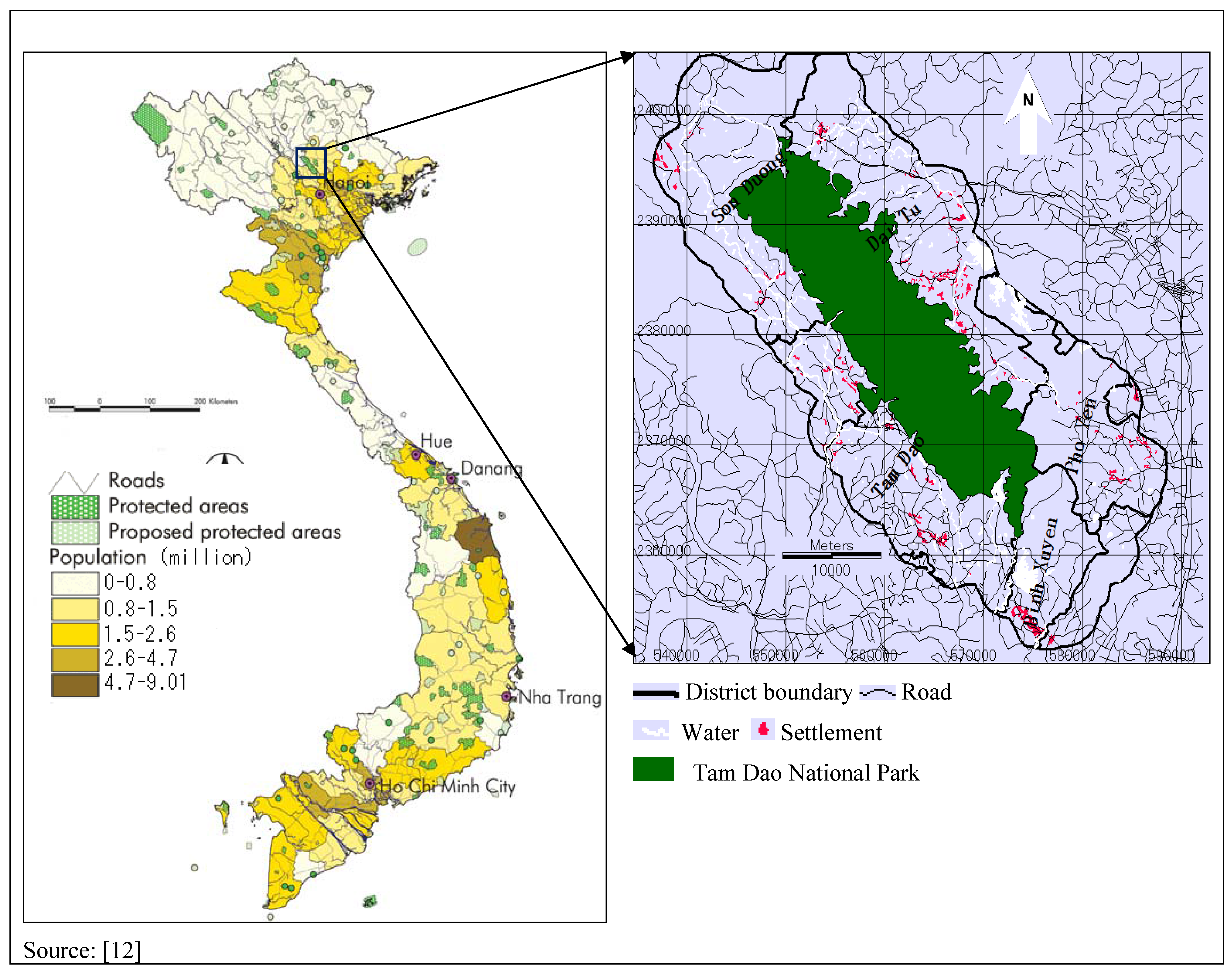
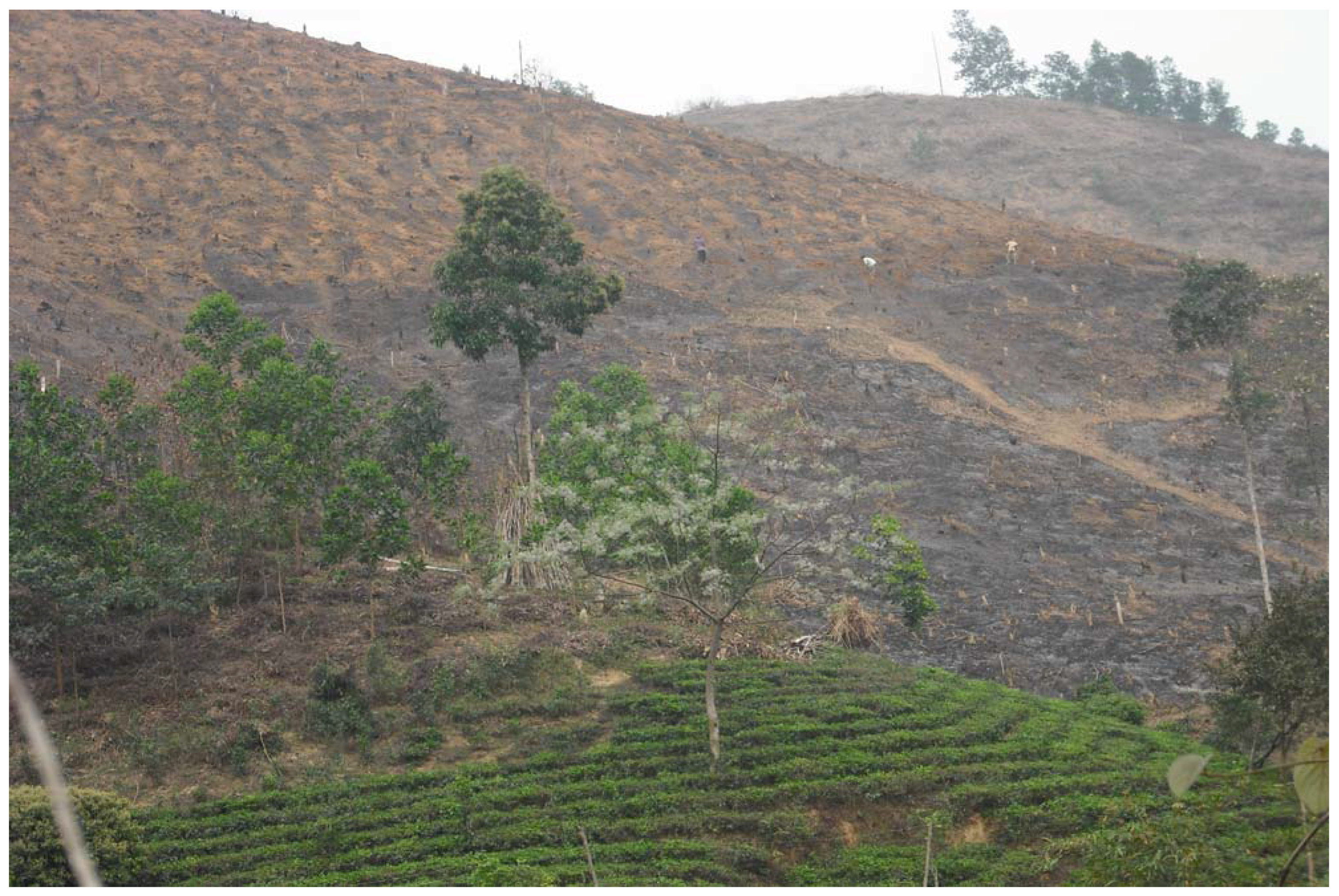
2.1. Study Area
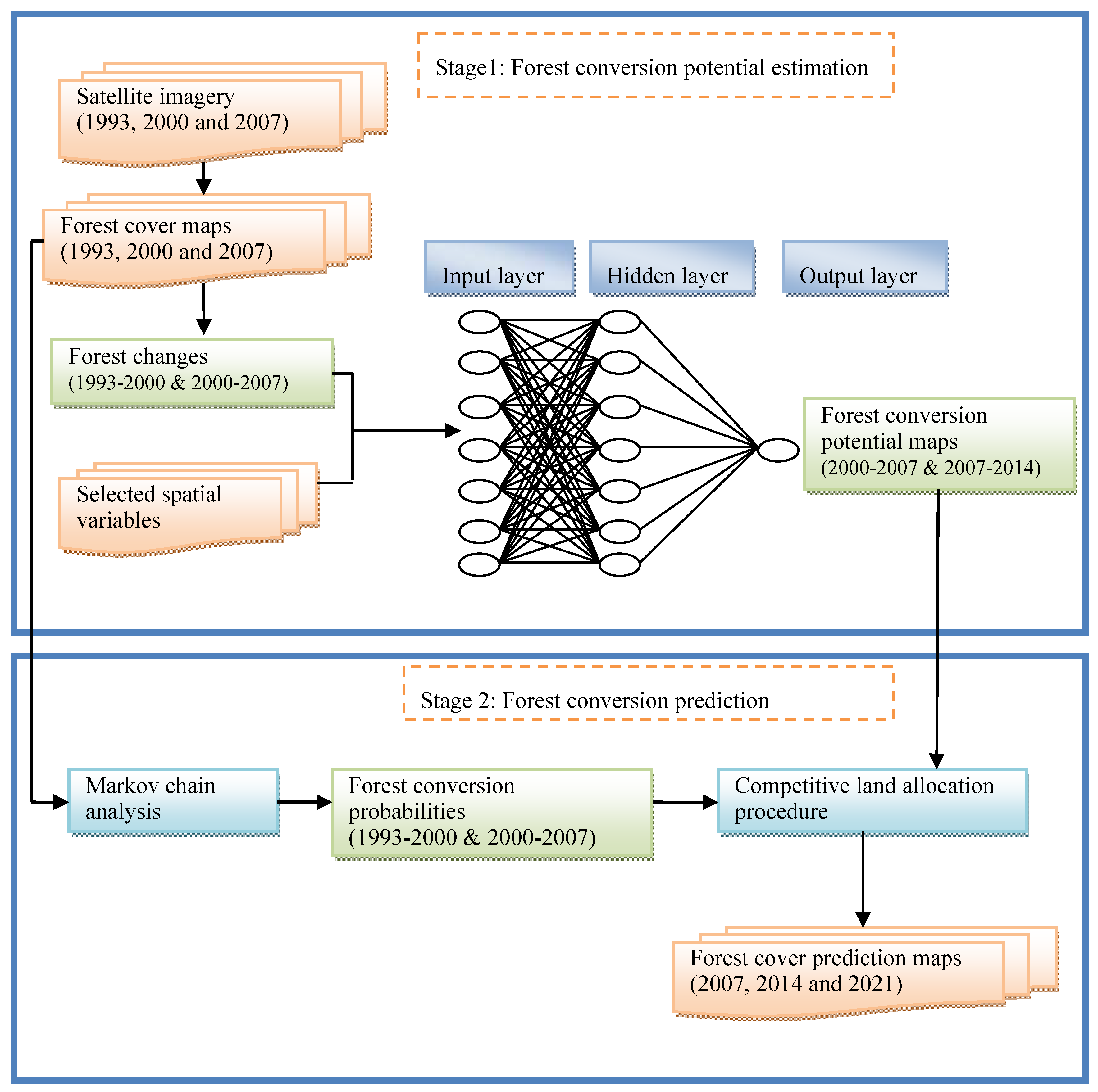
2.2. Implementation of the Multi-Layer Perceptron Neural Network and the Markov Model

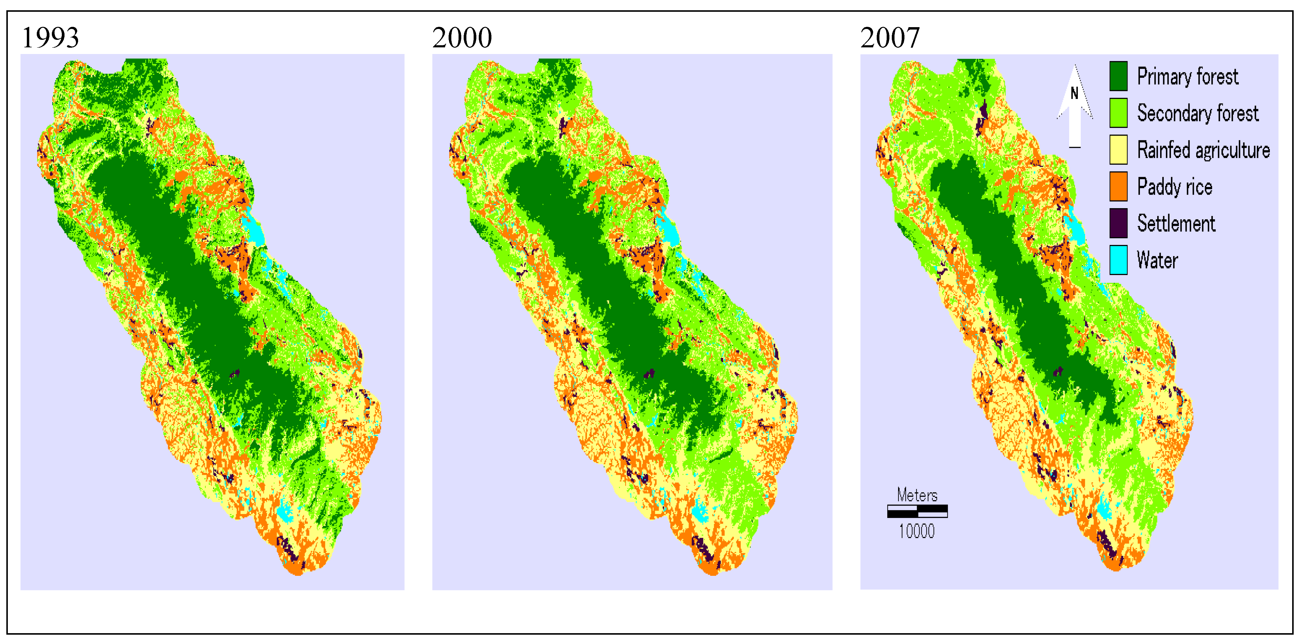
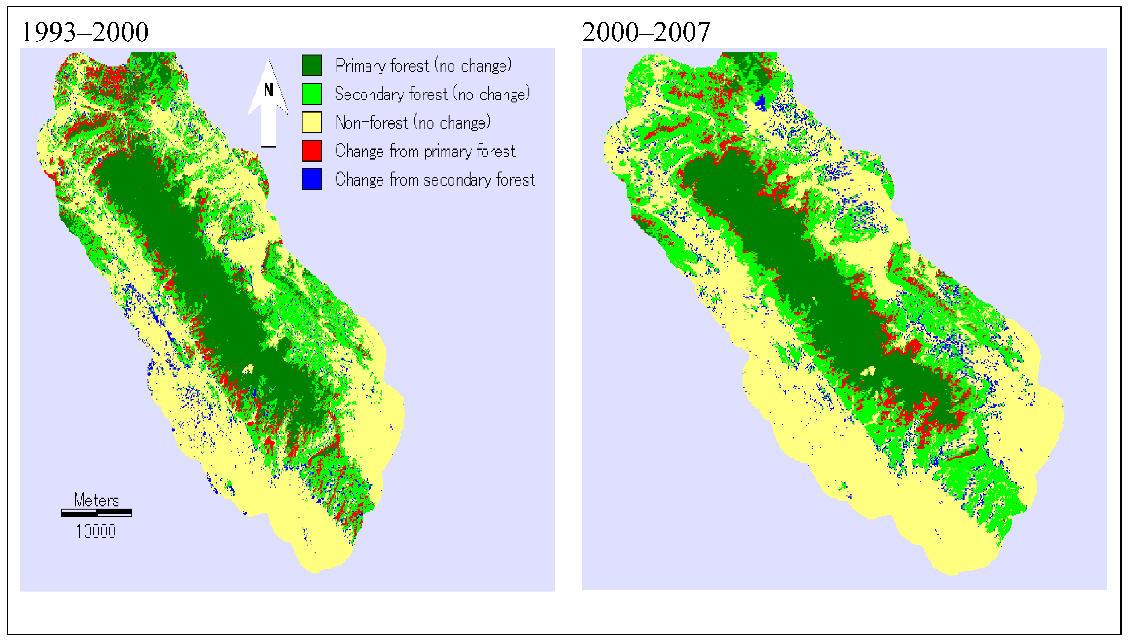
2.2.1. Observed Changes in Forest Cover Using Remotely Sensed Data
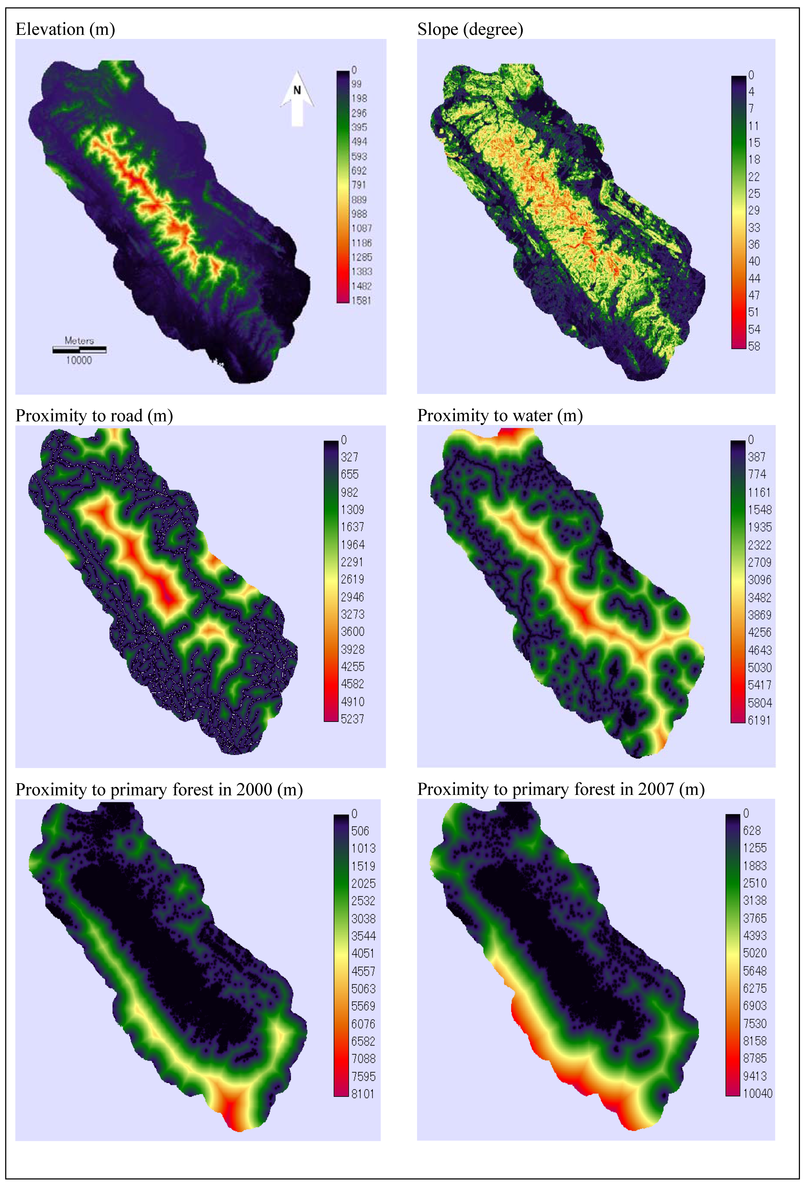
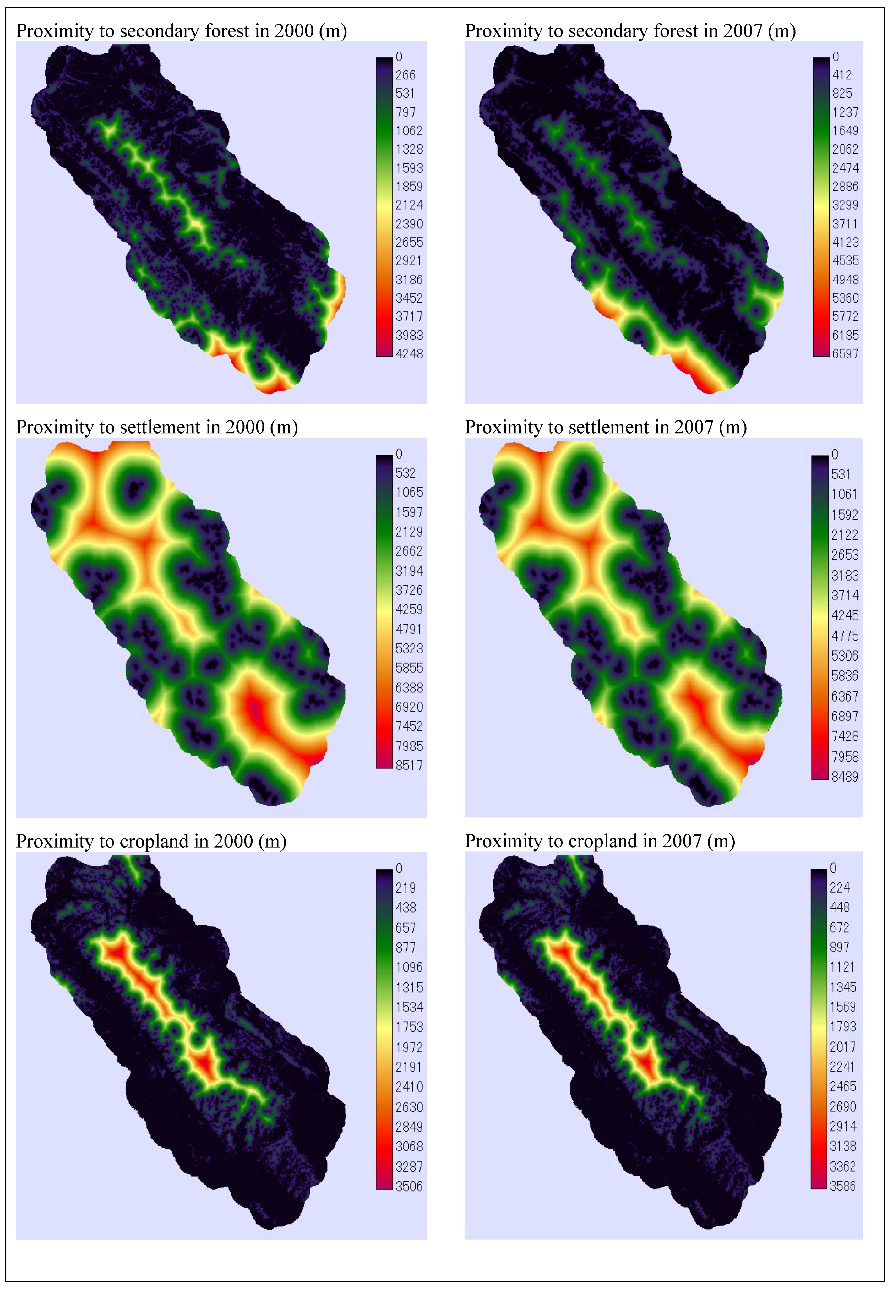
2.2.2. Selection of Spatial Variables

| Spatial variable | Mean | S.D. | Min. | Max. |
|---|---|---|---|---|
| Elevation (m) | 86 | 194 | 0 | 1,581 |
| Slope (degree) | 6.2 | 11.5 | 0 | 58 |
| Proximity to road (m) | 403 | 802 | 0 | 5,237 |
| Proximity to water (m) | 616 | 1,050 | 0 | 6,191 |
| Proximity to primary forest in 2000 (m) | 477 | 1,038 | 0 | 8,101 |
| Proximity to primary forest in 2007 (m) | 770 | 1,673 | 0 | 10,040 |
| Proximity to secondary forest in 2000 (m) | 146 | 406 | 0 | 4,248 |
| Proximity to secondary forest in 2007 (m) | 246 | 696 | 0 | 6,598 |
| Proximity to settlement in 2000 (m) | 1,169 | 1,818 | 0 | 8,517 |
| Proximity to settlement in 2007 (m) | 1,113 | 1,747 | 0 | 8,489 |
| Proximity to cropland in 2000 (m) | 122 | 392 | 0 | 3,506 |
| Proximity to cropland in 2007 (m) | 130 | 288 | 0 | 3,586 |
2.2.3. Forest Conversion Potential Estimation


2.2.4. Prediction of Forest Conversion for Identifying Vulnerable Areas
| 1993–2000 | Cramer’s V | 2000–2007 | Cramer’s V |
|---|---|---|---|
| Conversion from primary forest to secondary forest | |||
| Proximity to settlement in 2000 | 0.3459 | Proximity to settlement in 2007 | 0.3302 |
| Proximity to water | 0.5903 | Proximity to water | 0.6431 |
| Slope | 0.7053 | Slope | 0.6843 |
| Elevation | 0.7161 | Elevation | 0.7680 |
| Proximity to road | 0.8082 | Proximity to road | 0.8582 |
| Proximity to primary forest in 2000 | 0.9132 | Proximity to primary forest in 2007 | 0.9347 |
| Conversion from primary forest to cropland | |||
| Proximity to settlement in 2000 | 0.2911 | Proximity to settlement in 2007 | 0.2525 |
| Proximity to road | 0.3204 | Proximity to road | 0.2750 |
| Elevation | 0.4289 | Elevation | 0.4471 |
| Slope | 0.5014 | Slope | 0.4938 |
| Proximity to water | 0.5700 | Proximity to water | 0.5701 |
| Proximity to cropland in 2000 | 0.6552 | Proximity to cropland in 2007 | 0.6986 |
| Proximity to primary forest in 2000 | 0.8139 | Proximity to primary forest in 2007 | 0.8087 |
| Conversion from secondary forest to cropland | |||
| Proximity to settlement in 2000 | 0.3811 | Proximity to settlement in 2007 | 0.3536 |
| Proximity to road | 0.4101 | Proximity to road | 0.3652 |
| Elevation | 0.5089 | Elevation | 0.5473 |
| Slope | 0.6012 | Slope | 0.5835 |
| Proximity to water | 0.6803 | Proximity to water | 0.6903 |
| Proximity to cropland in 2000 | 0.7554 | Proximity to cropland in 2007 | 0.7961 |
| Proximity to secondary forest in 2000 | 0.8935 | Proximity to secondary forest in 2007 | 0.8743 |
3. Results
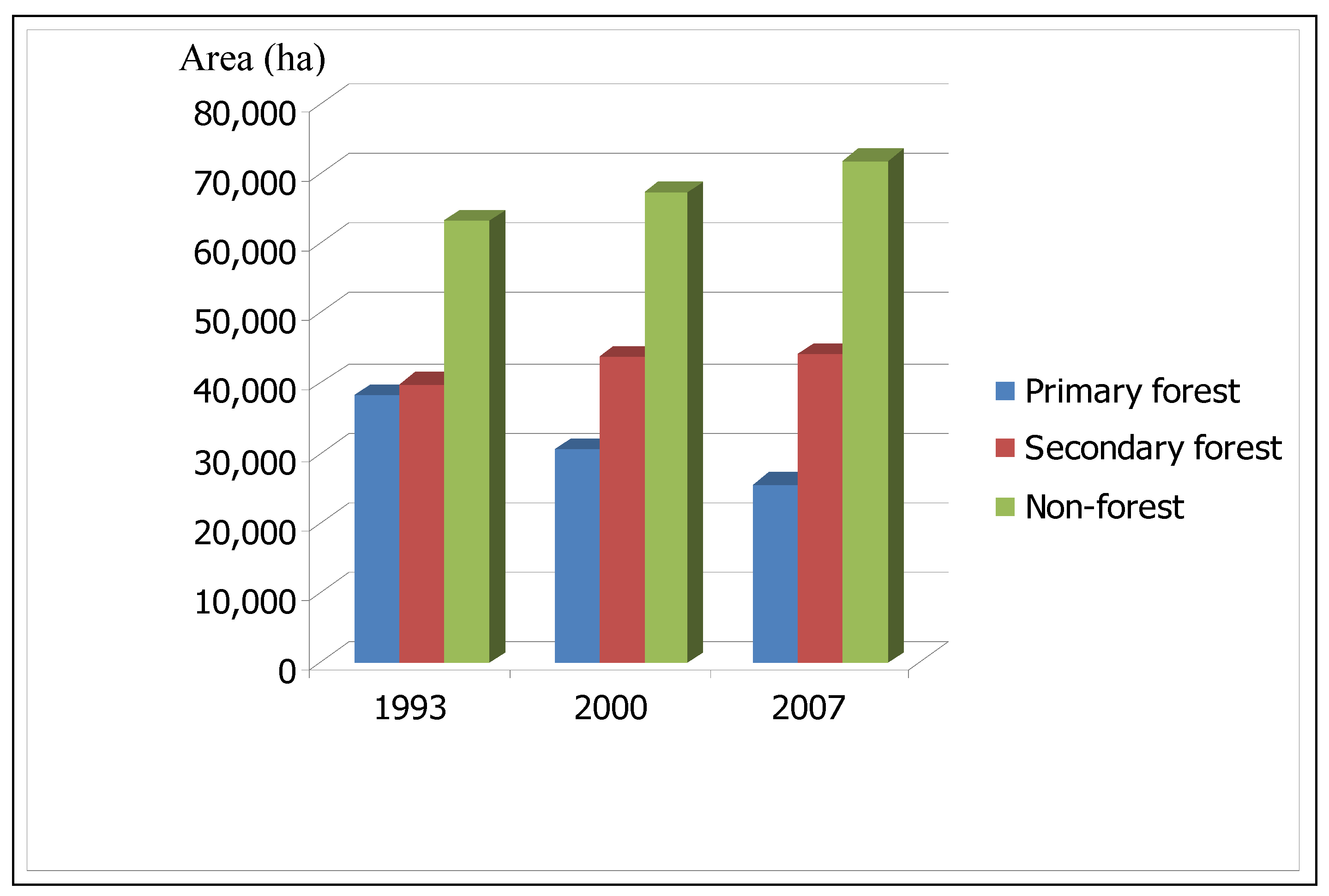
3.1. Observed Changes in Forest Cover


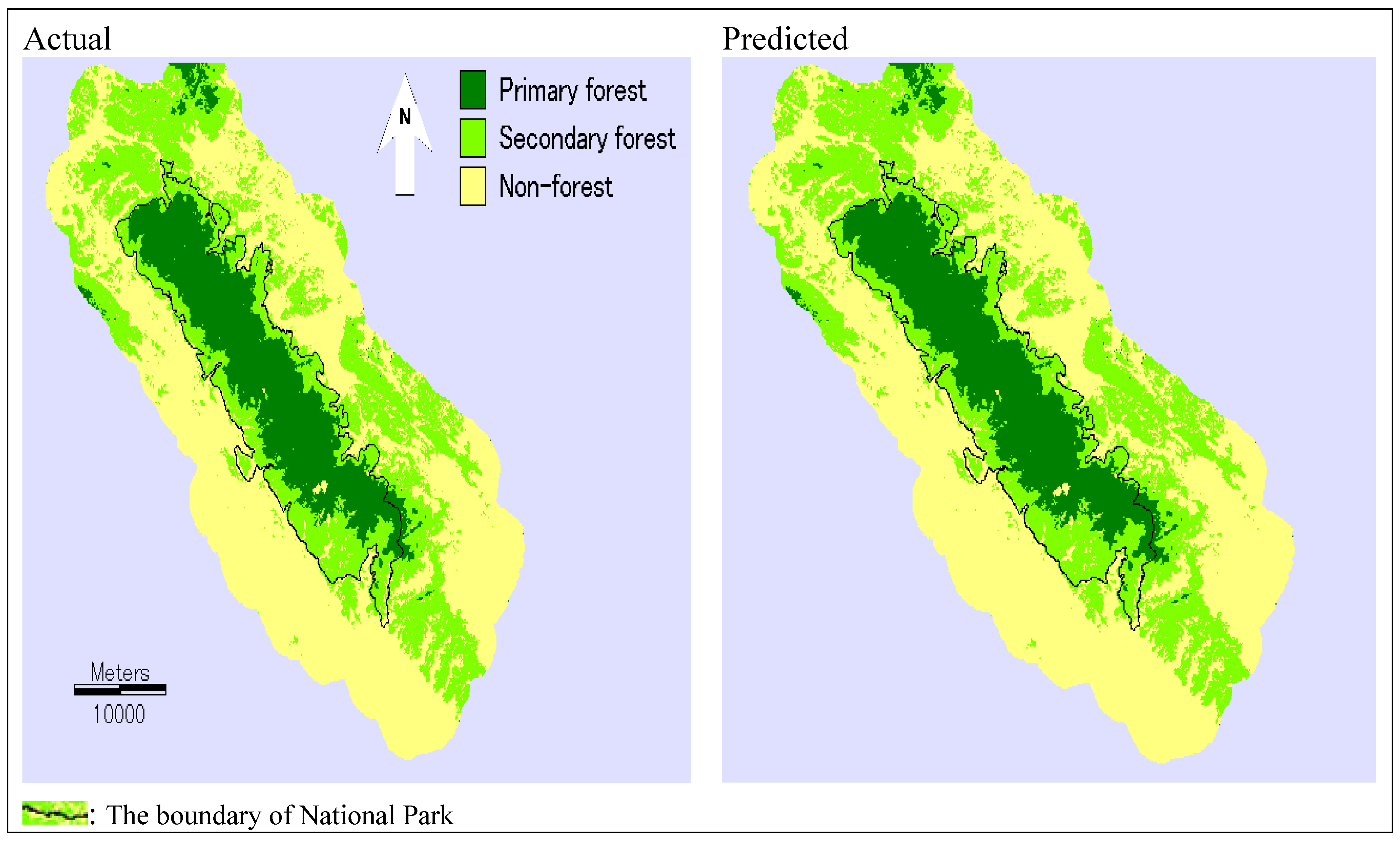
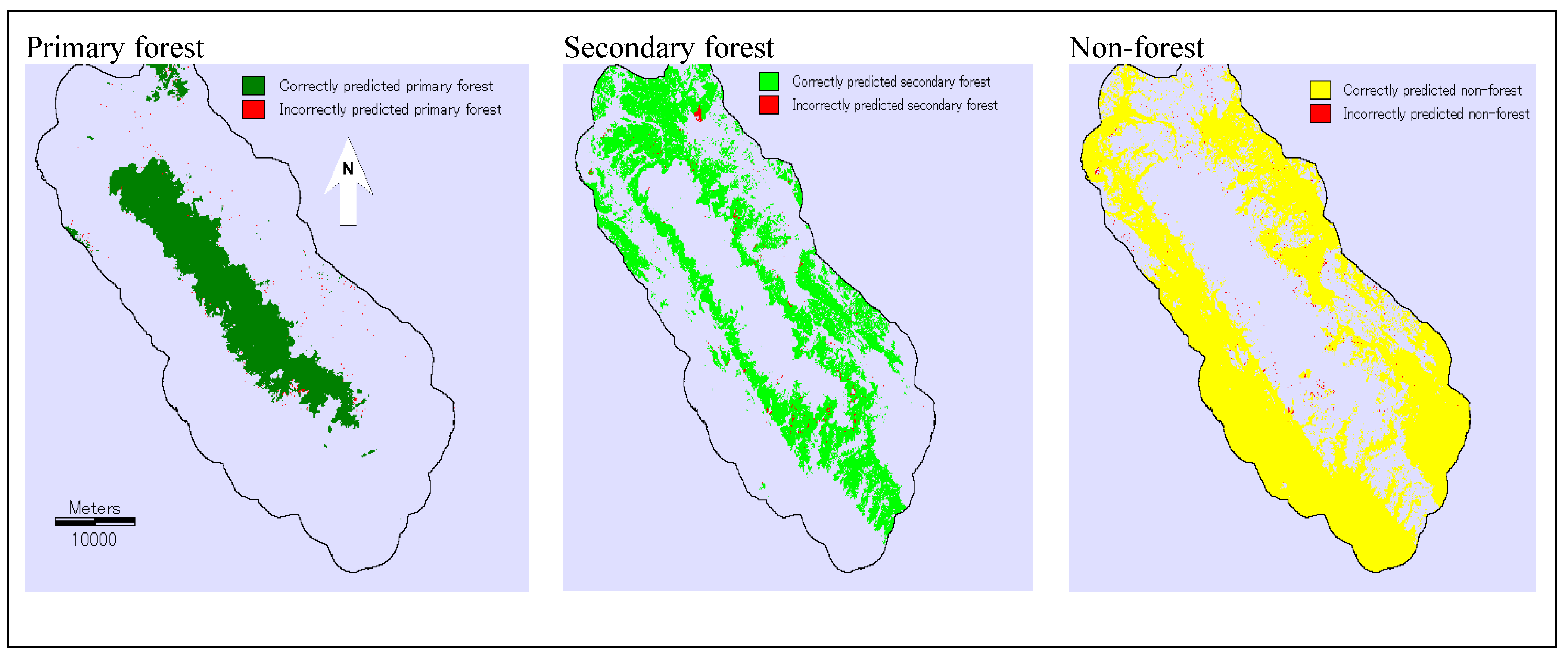
3.2. Model Validation
| Components of agreement and disagreement | The null model | The predicted model |
|---|---|---|
| Agreement due to chance | 33 | 33 |
| Agreement due to quantity | 6 | 7 |
| Agreement due to location | 53 | 56 |
| Disagreement due to location | 3 | 3 |
| Disagreement due to quantity | 5 | 1 |
| Category | Primary forest | Secondary forest | Non-forest |
|---|---|---|---|
| Primary forest | 0.7941 | 0.1959 | 0.0100 |
| Secondary forest | - | 0.9072 | 0.0928 |
| Non-forest | - | - | 1.0000 |
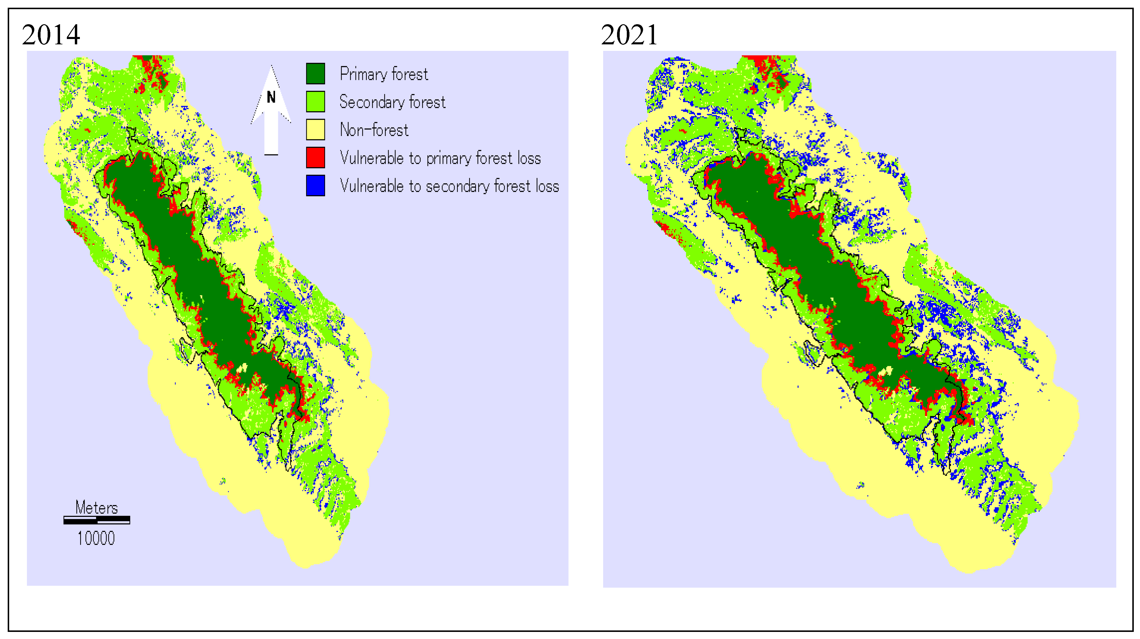
3.3. Areas Vulnerable to Future Forest Conversions
| Category | Primary forest | Secondary forest | Non-forest |
|---|---|---|---|
| Primary forest | 0.8379 | 0.1527 | 0.0094 |
| Secondary forest | - | 0.9026 | 0.0974 |
| Non-forest | - | - | 1.0000 |


| Category | 1993 | 2000 | 2007 (Real) | 2007 (Predicted) | 2014 | 2021 |
|---|---|---|---|---|---|---|
| Primary forest | 27.06 | 21.49 | 18.03 | 16.82 | 15.10 | 12.66 |
| Secondary forest | 28.21 | 30.89 | 31.17 | 32.60 | 30.88 | 30.18 |
| Non-forest | 44.73 | 47.62 | 50.81 | 50.58 | 54.01 | 57.16 |
4. Discussion
5. Conclusions
Acknowledgments
References and Notes
- Vitousek, P.M. Beyond global warming: ecology and global change. Ecology 1994, 75, 1861–1876. [Google Scholar] [CrossRef]
- Walker, R. Theorizing land-cover and land-use change: the case of tropical deforestation. Int. Reg. Sci. Rev. 2004, 27, 247–270. [Google Scholar] [CrossRef]
- Haines-Young, R. Land use and biodiversity relationships. Land Use Policy 2009, 26, 178–186. [Google Scholar] [CrossRef]
- Sala, O.E.; Chapin, F.S., III; Armesto, J.J.; Berlow, E.; Bloomfield, J.; Dirzo, R.; Huber-Sanwald, E.; Huenneke, L.F.; Jackson, R.B.; Kinzig, A.; Leemans, R.; Lodge, D.M.; Mooney, H. A.; Oesterheld, M.; Poff, N.L.; Sykes, M.T.; Walker, B.H.; Walker, M.; Wall, D.H. Global biodiversity scenarios for the year 2100. Science 2000, 287, 1770–1774. [Google Scholar] [CrossRef] [PubMed]
- Myers, N.; Mittermeier, R.A.; Mittermeier, C.G.; da Fonseca, G.A.B.; Kent, J. Biodiversity hotspots for conservation priorities. Nature 2000, 403, 853–858. [Google Scholar] [CrossRef] [PubMed]
- FAO (Food and Agriculture Organization of the United Nations). Global Forest Resources Assessment 2005: Progress toward Sustainable Forest Management; FAO: Rome, Italy, 2006; Available online: http://www.fao.org/DOCREP/008/a0400e/a0400e00.htm (accessed on 25 September 2008).
- Poffenberger, M.; Nguyen, H.P. Stewards of Vietnam’s Upland Forests; Center for Southeast Asia Studies: Berkeley, CA, USA, 1998; pp. 1–18. Available online: http://www.mekonginfo.org/mrc_en/doclib.nsf/0/E5E0A84E9B42A19F80256690003862FB/$FILE/FULLTEXT.html (accessed on 20 September 2008).
- Do Dinh Sam. Shifting Cultivation in Vietnam: Social, Economic and Environmental Values Relative to Alternative Land Use; International Institute for Environment and Development: London, UK, 1994; pp. 3–15. [Google Scholar]
- Meyfroidt, P.; Lambin, F.E. The causes of the reforestation in Vietnam. Land Use Policy 2008, 25, 182–197. [Google Scholar] [CrossRef]
- World Bank. World Development Report 1992: Development and the Environment; Oxford University Press: Madison, NY, USA, 1992; p. 200. Available online: http://econ.worldbank.org/external/default/main?pagePK=64165259&theSitePK=469372&piPK=64165421&menuPK=64166093&entityID=000178830_9810191106175 (accessed on 12 June, 2009).
- ICEM (International Centre for Environmental Management). Vietnam National Report on Protected Areas and Development; ICEM: Indooroopilly, Queensland, Australia, 2003; pp. 19–47. [Google Scholar]
- TDMP (Tam Dao National Park and Buffer Zone Management Project). Rural Household Economics Baseline Survey; Tam Dao National Park: Vietnam; Available online: http://tamdaonp.com.vn/ (accessed on 15 October 2009).
- Linkie, M.; Smith, R.J.; Leader-Williams, N. Mapping and predicting deforestation patterns in the lowlands of Sumatra. Biodivers. Conserv. 2004, 13, 1809–1818. [Google Scholar] [CrossRef]
- Giriraj, A.; Irfan-Ullah, M.; Murthy, M.S.A.; Beierkuhnlein, A. Modelling spatial and temporal forest cover change patterns (1973–2020): A case study from South Western Ghats (India). Sensors 2008, 8, 6132–6153. [Google Scholar] [CrossRef]
- Turner, W.; Spector, S.; Gardiner, N.; Fladeland, M.; Sterling, E.; Steininger, M. Remote sensing for biodiversity science and conservation. Trends Ecol. Evol. 2003, 18, 306–314. [Google Scholar] [CrossRef]
- Lambin, E.F. Modelling and monitoring land-cover change processes in tropical regions. Prog. Phys. Geog. 1997, 21, 375–393. [Google Scholar] [CrossRef]
- Khang, N.D.; Hoe, H.; Duc, H.D.; Thin, N.N.; Tien, D.D.; Lanh, V.L.; Huyen, T.H. Tam Dao National Park; Agricultural Publishing House: Hanoi, Vietnam, 2007; pp. 9–56. (in Vietnamese) [Google Scholar]
- Lambin, E.F. Modelling Deforestation Processes: A Review; TREES Series B: Research Report No. 1; EUR 15744 EN, European Commission: Luxembourg, 1994. [Google Scholar]
- Mas, J.F.; Puig, H.; Palacio, J.L.; Lopez, A.S. Modelling deforestation using GIS and artificial neural networks. Environ. Model. Software 2004, 19, 461–471. [Google Scholar] [CrossRef]
- Eastman, J.R. IDRISI Taiga, Guide to GIS and Remote Processing; Clark University: Worcester, MA, USA, 2009; pp. 234–256. [Google Scholar]
- Lek, S.; Delacoste, M.; Baran, P.; Dimopoulos, I.; Lauga, J.; Aulanier, S. Application of neural networks to modelling non-linear relationships in ecology. Ecol. Model. 1996, 90, 39–52. [Google Scholar] [CrossRef]
- Yuan, H.; Van Der Wiele, C.F.; Khorram, S. An automated artificial neural network system for land use/land cover classification from Landsat TM imagery. Remote Sens. 2009, 1, 243–265. [Google Scholar] [CrossRef]
- Zhou, J.; Civco, D. Using genetic learning neural networks for spatial decision making in GIS. Photogramm. Eng. Remote Sens. 1996, 62, 1287–1295. [Google Scholar]
- Ghazoul, J. Tam Dao Nature Reserve: Results of a Biological Survey; Society for Environmental Exploration, UK and Xuan Mai Forestry College: Hanoi, Vietnam, 1994. [Google Scholar]
- Eastman, J.R.; Jin, W.; Kyem, P.A.K.; Toledano, R. Raster procedures for multi-criteria/multi-objective decisions. Photogramm. Eng. Remote Sens. 1995, 61, 539–547. [Google Scholar]
- Pijanowski, B.C.; Brown, D.G.; Shellito, B.A.; Manik, G.A. Using neural networks and GIS to forescast land use changes: a land transformation model. Comput. Environ. Urban. 2002, 26, 553–575. [Google Scholar] [CrossRef]
- Li, X.; Yeh, A.G.O. Neural-network-based cellular automata for simulating multiple land use changes using GIS. Int. J. Geogr. Inf. Sci. 2002, 16, 323–343. [Google Scholar] [CrossRef]
- Dendoncker, N.; Roundsevell, M.; Bogaert, P. Spatial analysis and modeling of land use distributions in Belgium. Comput. Environ. Urban. 2007, 31, 188–205. [Google Scholar] [CrossRef]
- Ali, J.; Benjaminsen, A.T.; Hammad, A.A.; Dick, B.O. The road to deforestation: An assessment of forest loss and its causes in Basho Valley, Nothern Pakistan. Global Environ. Change 2005, 15, 370–380. [Google Scholar] [CrossRef]
- Cropper, M.; Puri, J.; Griffiths, C. Predicting the location of deforestation: the role of roads and protected areas in North Thailand. Land Econ. 2001, 77, 172–186. [Google Scholar] [CrossRef]
- Wilkie, D.; Shaw, E.; Rotberg, F.; Morelli, G.; Auzel, P. Roads, development, and conservation in the Congo Basin. Conserv. Biol. 2000, 14, 1614–1622. [Google Scholar] [CrossRef]
- Ludeke, A.K.; Maggio, R.C.; Reid, L.M. An analysis of anthropogenic deforestation using logistic regression and GIS. J. Environ. Manag. 1990, 1, 247–259. [Google Scholar] [CrossRef]
- De Koninck, R. Deforestation in Vietnam; International Development Research Center: Ottawa, Canada, 1999; Available online: http://www.idrc.ca/en/ev-9318-201-1-DO_TOPIC.html (accessed on 15 September 2008).
- Sader, S.A.; Joyce, A.T. Deforestation rates and trends in Costa Rica, 1940–1983. Biotropica 1998, 20, 11–19. [Google Scholar] [CrossRef]
- Kanellopoulos, I.; Wilkinson, G.G. Strategies and best practice for neural network image classification. Int. J. Remote Sens. 1997, 18, 711–725. [Google Scholar] [CrossRef]
- Pontius, R.G.; Huffaker, D.; Denman, K. Useful techniques of validation for spatially explicit land change models. Eco.Model. 2004, 179, 445–461. [Google Scholar] [CrossRef]
- Brown, S.; Lugo, A.E. Tropical secondary forests. J. Trop. Ecol. 1990, 6, 1–32. [Google Scholar] [CrossRef]
- Wright, S.J. Tropical forests in a changing environment. Trends Ecol. Evol. 2005, 20, 553–560. [Google Scholar] [CrossRef] [PubMed]
- Bawa, K.S.; Dayanandan, S. Socioeconomic factors and tropical deforestation. Nature 1997, 386, 562–563. [Google Scholar] [CrossRef]
- Merten, B.; Lambin, E.F. Spatial modeling of tropical deforestation in southern Cameroon: spatial disaggregation of diverse deforestation processes. Appl. Geog. 1997, 17, 143–162. [Google Scholar] [CrossRef]
- Geist, H.J.; Lambin, E.F. Proximate causes and underlying driving forces of tropical deforestation. BioScience 2002, 52, 143–150. [Google Scholar] [CrossRef]
- Kuznetsov, A.N. Rapid Botanical Assessment of Tam Dao National Park: Detailed Botanical Survey Final Report; Tam Dao National Park: Tam Dao, Vietnam, 2005. [Google Scholar]
© 2010 by the authors; licensee MDPI, Basel, Switzerland. This article is an open-access article distributed under the terms and conditions of the Creative Commons Attribution license (http://creativecommons.org/licenses/by/3.0/).
Share and Cite
Khoi, D.D.; Murayama, Y. Forecasting Areas Vulnerable to Forest Conversion in the Tam Dao National Park Region, Vietnam. Remote Sens. 2010, 2, 1249-1272. https://doi.org/10.3390/rs2051249
Khoi DD, Murayama Y. Forecasting Areas Vulnerable to Forest Conversion in the Tam Dao National Park Region, Vietnam. Remote Sensing. 2010; 2(5):1249-1272. https://doi.org/10.3390/rs2051249
Chicago/Turabian StyleKhoi, Duong Dang, and Yuji Murayama. 2010. "Forecasting Areas Vulnerable to Forest Conversion in the Tam Dao National Park Region, Vietnam" Remote Sensing 2, no. 5: 1249-1272. https://doi.org/10.3390/rs2051249
APA StyleKhoi, D. D., & Murayama, Y. (2010). Forecasting Areas Vulnerable to Forest Conversion in the Tam Dao National Park Region, Vietnam. Remote Sensing, 2(5), 1249-1272. https://doi.org/10.3390/rs2051249