Description and Performance of an L-Band Radiometer with Digital Beamforming

Abstract

This paper presents the description and performance tests of an L-band microwave radiometer with Digital Beamforming (DBF), developed for the Passive Advanced Unit (PAU) for ocean monitoring project. PAU is an instrument that combines, in a single receiver and without time multiplexing, a microwave radiometer at L-band (PAU-RAD) and a GPS-reflectometer (PAU-GNSS-R). This paper focuses on the PAU‑RAD beamformer’s first results, analyzing the hardware and software required for the developed prototype. Finally, it discusses the first results measured in the Universitat Politècnica de Catalunya (UPC) anechoic chamber.

1. Introduction

The interest of the scientific community in remotely measuring Sea Surface Salinity (SSS) has been increasing in recent years and much effort has been spent in that direction by the European Space Agency (ESA) and the National Aeronautics and Space Administration (NASA) with the MIRAS/SMOS [1] and the AQUARIUS/SAC-D [2] missions, respectively. In principle, a number of radiometer architectures are suitable to be used for SSS retrieval applications, but the radiometric accuracy and sensitivity requirements are very challenging constraints (ΔT_B ~ 0.1 K). In this regard, one of the major concerns of a radiometer design is its radiometric sensitivity that can be improved using low noise devices or even operating in a cool temperature environment. Furthermore, to achieve these tough requirements, several auxiliary techniques can be used depending of the sensor type, not necessarily related to the radiometer design. For ground-based measurements, the radiometric resolution can be improved simply by increasing the integration time as long as needed, due to the stationary nature of the measurements. This, however, is not possible for airborne or spaceborne sensors. In this case, one option is to acquire multi-angular measurements of the same scene, taking advantage of the well-known dependence of the emissivity on the polarization and the incidence angle [3] (Figure 1).

Figure 1. Vertical and horizontal emissivities vs. incidence angle. PAU-RAD antenna boresight pointed at 45° and with the digital beamforming signal processing technique creates beams from 30° to 60° incidence angles in 5° steps. The emissivity curve corresponds to a calm sea with T_sea = 293 K, SSS = 36 psu and at f_GPS‑L1 = 1,575.42 MHz.

Figure 1. Vertical and horizontal emissivities vs. incidence angle. PAU-RAD antenna boresight pointed at 45° and with the digital beamforming signal processing technique creates beams from 30° to 60° incidence angles in 5° steps. The emissivity curve corresponds to a calm sea with T_sea = 293 K, SSS = 36 psu and at f_GPS‑L1 = 1,575.42 MHz.

Knowing this angular and polarization dependence, it is possible to merge these measurements to retrieve geophysical parameters with a reduced standard deviation. This can be done using theoretical or semi-empirical models and minimizing a cost function following a non-linear least-squares estimation algorithm, such as the Levenberg-Marquardt algorithm [4]. If the measurements’ noise is uncorrelated, the standard deviation of the estimated observable is reduced to $\sqrt{N}$, where N is the number of independent measurements. If measurements are not uncorrelated, the standard deviation decreases less rapidly following different trends [5].

Typically, brightness temperature measurements at different incidence angles can be obtained simultaneously using different receivers, or with the same receiver acquiring data at different times [6,7]. Furthermore, multi-angular measurements are inherent in the image formation process in synthetic aperture radiometers such as SMOS/MIRAS [8] or PAU-Synthetic Aperture (PAU-SA) [9]. This paper presents a new option to obtain multi-angular measurements combining an L-band radiometer with the concept of digital beamformer (DBF), which is able to steer multiple and simultaneous beams at different incidence angles without mechanical scan. This work focuses on the design, first results and performance of using digital beamforming techniques applied to an L-band radiometer.

2. PAU-RAD Overview

The Passive Advanced Unit (PAU) for ocean monitoring [10] is an instrument that combines, in a single receiver and without time-multiplexing, an L-band microwave radiometer (PAU-RAD) [11] and a GPS-reflectometer (PAU-GNSS/R) [12,13,14] which, in conjunction with an infra-red radiometer (PAU-IR) [15], simultaneously provide the sea state information and surface temperature needed to accurately retrieve the SSS. Furthermore, PAU-RAD, as it has been designed, is a concept demonstrator ground-based instrument, which is expected to measure multi-angular incidence ocean brightness temperature from a terrain elevation, for instance a cliff. Measurements of the ocean brightness temperature from a cliff have previously been successfully conducted, such as in [14], where the height above sea level was 110 meters.

PAU-RAD is a digital radiometer with DBF and polarization synthesis capabilities. That is, any polarization can be generated by a proper combination of signals collected by the two orthogonal polarizations of the antenna. The DBF consists of a 4 × 4 rectangular array with triangular illumination. A simplified sketch of the PAU-RAD architecture is presented in Figure 2, where:

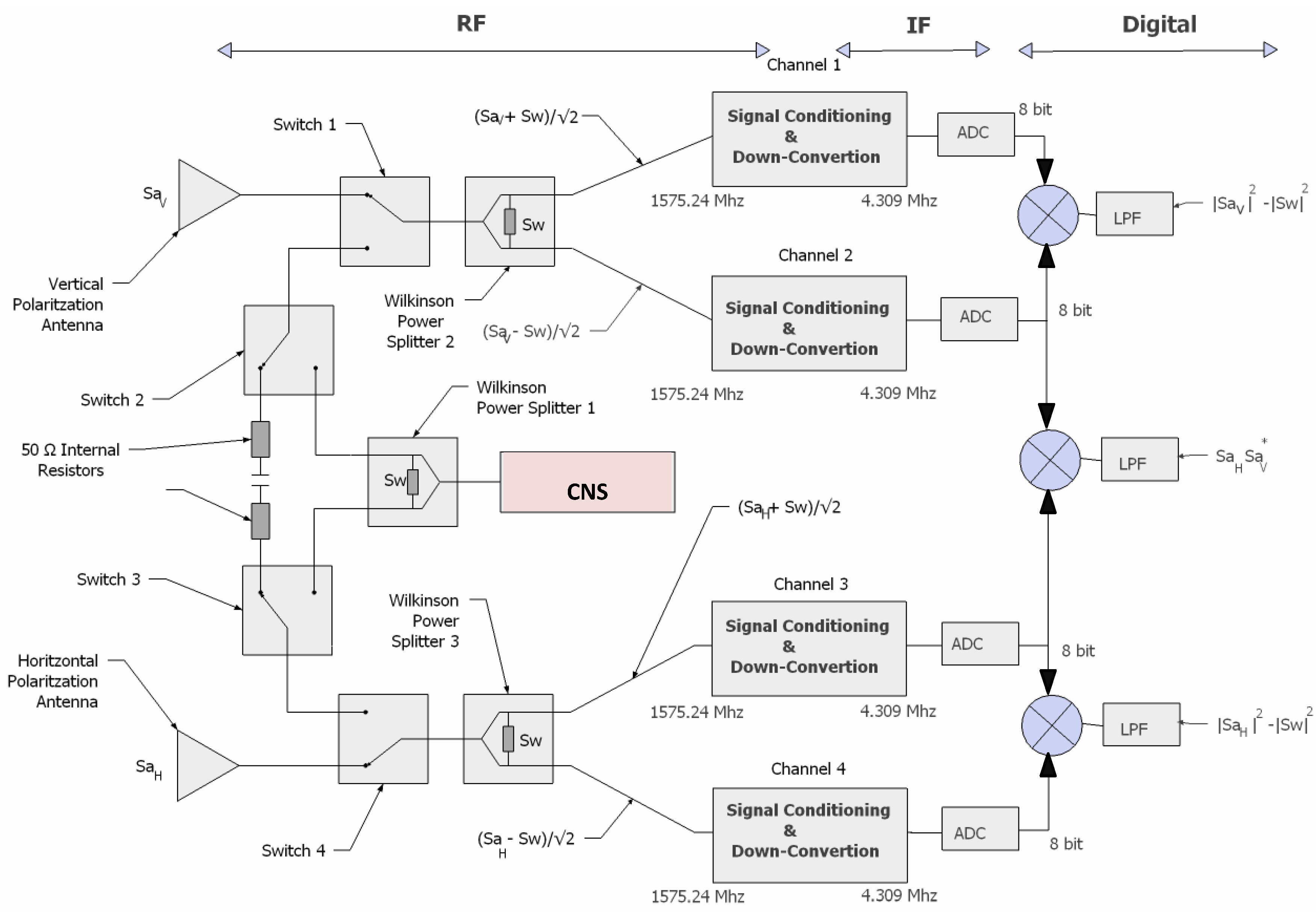
• S_aVH, S_w are the antenna signal, from vertical and horizontal polarization, and the Wilkinson’s signal, respectively;
• CNS stands for Controlled Noise Source; and
• LPF stands for Low Pass Filter.

The PAU-RAD radiometric architecture is based on a new kind of correlation radiometer (Figure 2) equivalent to a Dicke radiometer in terms of radiometric output (α $T_a-T_w$) and to a total power radiometer in terms of radiometric sensitivity ($T_{sys}/\sqrt{B\tau }$) [10], where $T_a$ is the antenna temperature, $T_w$ is the temperature of the Wilkinson’s power splitter, $T_{sys}=(T_a+T_w)/2+T_{REC}$ is the system temperature, $T_{REC}$ is the receiver noise temperature and $B\tau$ is the product of the equivalent noise bandwidth with the integration time.

To clarify the PAU-RAD radiometric concept, Figure 2 shows a simplified model, which uses only a dual-polarization receiver and two channels per polarization (a total of four channels per receiver). The outputs of the PAU-RAD are the complex correlation between the signals at the outputs of a Wilkinson power splitter (upper and lower channels), which are proportional to the antenna temperature minus the Wilkinson’s resistor physical temperature. Since the output is a complex value, it has modulus and phase. The phase of this complex value is the differential phase between both channels and is zero only if the upper and lower channels have exactly the same phase. Otherwise, the resulting phase will be relevant for calibration purposes (Section 3.2). The correlation of the signals from the two orthogonal polarizations is proportional to the third (real part) and fourth (imaginary part) Stokes parameters. The results of PAU-RAD are the four Stokes parameters as it is a full-polarimetric radiometer. The Stokes parameters characterize the polarization status of a surface’s polarized brightness temperature. This polarization relates to different phenomena, such as the incidence angle, the SSS, the sea surface temperature, the sea surface roughness, wind direction and many others. The first and the second Stokes parameters are proportional to the sum and the difference of the brightness temperatures at vertical and horizontal polarizations. It is known that the sea surface salinity can be retrieved from these two parameters [3]. The third and the fourth parameters characterize the complex correlation between these two orthogonal polarizations [16].

Figure 2. PAU-RAD concept explained through a one element sketch. The antenna signal at each polarization is split in two by a Wilkinson power divider. The correlation of the channels of the same polarization is proportional to the antenna temperature minus the Wilkinson’s resistor physical temperature, as in the case of a Dicke radiometer. The correlation of the two channels of different polarizations is a complex value proportional to the third Stokes parameter (real part) and the fourth Stokes parameter (imaginary part).

Figure 2. PAU-RAD concept explained through a one element sketch. The antenna signal at each polarization is split in two by a Wilkinson power divider. The correlation of the channels of the same polarization is proportional to the antenna temperature minus the Wilkinson’s resistor physical temperature, as in the case of a Dicke radiometer. The correlation of the two channels of different polarizations is a complex value proportional to the third Stokes parameter (real part) and the fourth Stokes parameter (imaginary part).

A first analysis, using only one receiver demonstrator, of the PAU-RAD calibration algorithms and their performance was described in [11]. Then, the first results, analysis and digital beamforming antenna diagrams where presented in [17]. This work is the continuation, verification and extension of these preliminary works.

In Section 1, an introductory overview to the PAU concept has been given. Section 2 analyzes the PAU-RAD system. The digital beamforming is discussed in Section 3. Section 4 is devoted to the PAU-RAD instrument, focusing on hardware and software aspects. In Section 5 the first measurements of the beam steered by the DBF are presented. Finally, Section 6 summarizes the main conclusions of this work.

The PAU-RAD Instrument

Each of the 4 × 4 array elements (Figure 2) has a dual-polarization antenna (horizontal and vertical). Each polarization signal (S_aV and S_aH) is divided using a Wilkinson power splitter, followed by a pair of receiving channels (upper and lower ones). After signal conditioning at Radio Frequency (RF), the input signals are down-converted at an Intermediate Frequency (IF) of 4.309 MHz with a 2.2 MHz bandwidth (L1-GPS bandwidth). Once each channel is down-converted to IF, these signals are digitized at 8 bits using band-pass sampling techniques with a sampling frequency of 5.745 MHz. This frequency plan simplifies signal processing operations since the digital frequency is 0.25. Digitized signals are properly low-pass filtered, I/Q demodulated and processed in an ALTERA Field Programmable Gate Array (FPGA), where the full digital radiometer is embedded [11] (described in VHDL-97 digital description language [18]). Finally, after data calibration and through data processing, values proportional to the Stokes parameters can be achieved as follows: The first and the second Stokes parameters are obtained adding and subtracting the results of the same polarization channels correlation (Figure 2). On the other hand, the third and fourth parameters are twice the real and imaginary parts of the correlation of the two orthogonal polarizations.

To achieve the best performance, the L-band radiometer should operate in the 1,400–1,427 MHz “protected” band and the GPS reflectometer at 1,575.42 MHz (GPS-L1 band), where open C/A codes can be used to generate the local replicas of the GPS signal. However, in the PAU instrument demonstrator, the GPS reflectometer and the L-band radiometer share the same front-end: A commercial GPS down-converter (Zarlink GP2015 [19]). As a result, both operate at 1,575.42 MHz. This architecture reduces the required hardware resources, using only one RF-IF front end instead of two or a dual-band one for each receiver [20]. Although sharing the same RF-IF front-end provides a significant hardware reduction, the system has to deal with some incurred handicaps. The first one concerns the bandwidth, the radiometer uses only the 2.2 MHz GPS band, instead of the nearly 27 MHz available at the protected L-band. Obviously, it has an impact on the radiometric resolution, which can only be compensated by increasing the integration time. The second handicap concerns the interference that GPS signals can incur on the radiometric measurements. Although the spread‑spectrum modulation GPS signal is lower than the noise level (−27 dB below the noise level), the impact of the GPS interference on the radiometer measurements has to be quantified [11]. For this purpose, two extreme scenarios are distinguished considering a sea surface reflection coefficient of Γ = 0.7, a height of h = 110 m (the same height as in [14]) and an antenna’s effective area of A_eff = 0.16 m² (D = 17.5 dB, where D stands for antenna directivity) for both cases. The worst situation occurs when the specular reflection point is at the antenna’s boresight. In this case the antenna temperature increases due to the GPS interference is ∆T = 2.3 K (equivalent to ~4.6 psu salinity error in warm water). On the other hand, the best possible scenario occurs when the reflection point comes 90º out of boresight (and the attenuation due to the antenna pattern is ~15 dB), the radiometric measurement contribution is then ∆T ~ 0.03 K (~0.06 psu salinity error in warm water), below the 0.1 psu requirement of the Global Ocean Data Assimilation Experiment (GODAE) for open ocean [21]. Taking into account that the radiometer can create different beams using the DBF processing technique and that the specular reflection points are known and can be tracked, the chances of having a significant interference level are negligible.

3. Digital Beamforming General Considerations

DBF is a signal processing technique used in sensor arrays to steer the direction of the received signal. The technique is well known and widely used in communications systems and the remote sensing framework, even though to the authors’ knowledge this is the first time it is used in microwave radiometry. However, some studies and operative instruments using the related idea of phased array have been carried out [22], especially in the radio-astronomy field. Both concepts, digital beamforming and phased array, are similar, but some substantial differences exist. The phased array is based on the variation of the phase for each individual antenna in such a way the effective radiation pattern of the array is steered to the desired angle. In addition, the phase shifters typically used in phased arrays, introduce losses that degrade the noise figure, and therefore the radiometric resolution. On the other hand, DBF is the result of digital signal processing, which implies absolute reconfigurability. Furthermore, since each antenna signal is digitized, it is possible to obtain more than one beam simultaneously. In theory, a continuous scan can be performed obtaining an infinite number of beams simultaneously, only limited by the hardware requirements. These differences make the DBF more suitable for passive remote sensing applications.

A DBF is a spatial filter. Each antenna’s collected signals are properly weighted and added to get the system output. The system controls digitally the complex weight (phase and amplitude) of each antenna in order to attenuate some directions and reinforce some others, so it creates an interference pattern in the wavefront to steer the beam. The DBF implementation (Equation 1) is straightforward: each antenna’s signal is amplified, down-converted, sampled, weighted with a complex coefficient and, finally, added with the other antenna signals to get the DBF signal:

$$S_{DBF}^p(n,{\phi }_0,{\theta }_0)=\text{}{\displaystyle \sum _{m=1}^M{w}_m·S_{a_m}^p(n),}$$

(1)

where:

• $S_{DBF}^p(n,{\phi }_0,{\theta }_0)$ is the resulting signal of the digital beamforming steered to $({\phi }_0,{\theta }_0)$ at the n instant for the p polarization;
• $(\phi ,\theta )$ are the azimuth and zenith angles of the system;
• M is the total number of antennas distributed over a plane in a linear or planar array distribution;
• $w_m$ is the complex weight applied to the m^th antenna to steer the beam to $({\phi }_0,{\theta }_0)$; and
• $S_{a_m}^p(n)$ is the collected signal of the m^th antenna at the n instant and for the p polarization.

3.1. Calibration Errors that Can Be Handled by the PAU-RAD Array

Although DBF presents several clear advantages, it requires a previous hardware calibration. Signals to be combined by the DBF have to be previously calibrated in phase and amplitude. Thereby, since it is not possible to ensure this by system design, the whole receiver set has to be equalized in phase and amplitude. This point is a key issue to compose the digital array.

In PAU-RAD, analog receivers are driven from an ovenized 10 MHz master clock that is distributed to all receivers to generate their own local oscillator. Hence, it can be assumed that each receiver’s PLL has a fixed, but possibly slowly varying, random phase variable uniformly distributed within [0–2π). Furthermore, each receiver has a nominal 110 dB gain chain. Component tolerances can strongly affect this nominal gain. For this reason, each receiver has a potentiometer that controls the last amplifier stage at IF to manually equalize all receivers’ gain within 110 dB ± 1 dB. Even with this functionality, the gain has to be taken into consideration as a first approximation, a random variable with a normal probability density function with a standard deviation of 1 dB. The residual calibration errors will ultimately determine the quality of the synthesized array factor.

There are some figures of merit to measure the quality of an array. In this study the main beam efficiency (MBE) has been selected because it unifies different parameters (main beamwidth, side lobe levels (SLL), backside lobe, etc.) in a single one. In general, the MBE is defined as the ratio between the collected power by the main beam of the array and the collected total power. Theoretically, the main beam ends in the nulls between the main beam and the first side lobes, but in practice, these nulls are difficult to determine due to noise phase error and the angular resolution of the measurement system. In practice, to compute the edge of the main beam, it is considered that the main beam ends when it reaches the maximum side lobe amplitude level. In any case, this approximation gives a slightly lower MBE value than the real one.

For radiometric applications a high MBE is required (>90%) to ensure that the main contribution of the collected power comes from the main beam. In this case, the PAU-RAD MBE target is >94% to ensure, at least, the same performance as in previous developed radiometers [23].

Figure 3 shows the MBE degradation dependence with the residual calibration error for amplitude and phase, respectively. The determining parameter is the residual phase error, which corrupts the MBE rapidly. This is well known for radiometrics.

Figure 3. Degradation of the MBE vs. the amplitude (left) and phase (right) residual calibration error, obtained using theoretical development and simulations, pointing to the boresight. The considered array has 4 × 4 elements with triangular illumination.

Figure 3. Degradation of the MBE vs. the amplitude (left) and phase (right) residual calibration error, obtained using theoretical development and simulations, pointing to the boresight. The considered array has 4 × 4 elements with triangular illumination.

To fulfill the radiometric requirements, a MBE equal or higher to 0.94 has to be obtained. As shown in Figure 3, this can be fulfilled with a residual standard deviation error of 10º for the phase and 0.25 dB for the amplitude. Despite these residual values, more exigent residual standard deviation errors were selected as a calibration residual error target in order to ensure a high MBE. Actually, a residual standard deviation error of 2° for the phase and 0.1 dB for the amplitude were chosen as targets. These target values (2° and 0.1 dB) were already achieved in a preliminary work in which only one receiver was considered [11]. These are the specifications adopted for the whole hardware calibration performance. It is important to note that the phase and amplitude errors drift with temperature and time, so that hardware calibration needs to be periodically performed, each time the residual errors cross over these specified thresholds.

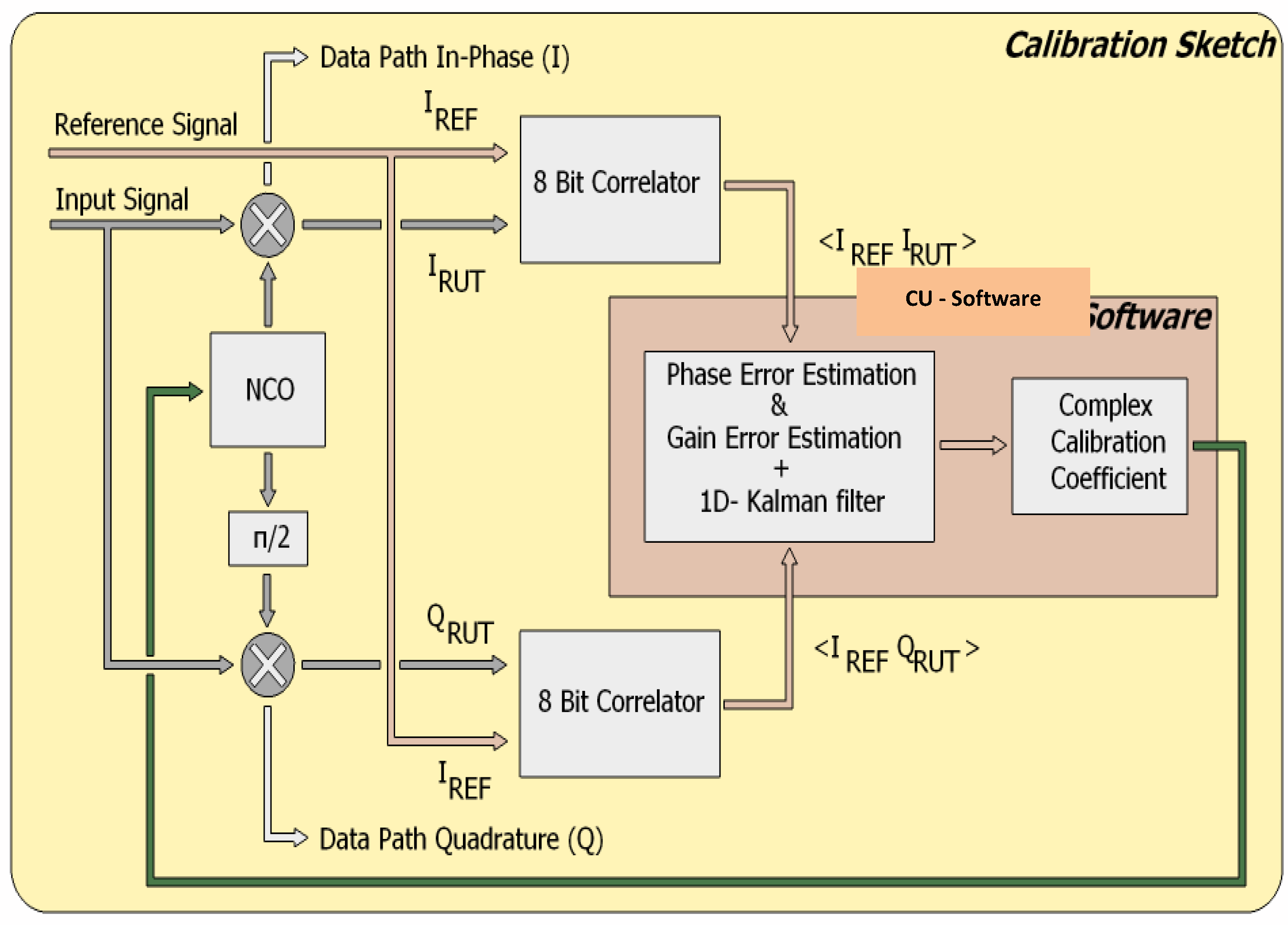
3.2. Amplitude and Phase Errors Estimation

A complex cross-correlation is used to estimate the amplitude and phase errors among receivers. The performance of the DBF requires only a relative calibration, that is having all the amplitudes and phases equalized. It does not require an absolute calibration, i.e., set all the phases to 0° and all the amplitudes to a predetermined value. To implement the relative calibration, a reference receiver is chosen, and the amplitude and phase of the other receivers are adjusted accordingly.

To estimate the errors, all receivers have to be driven by the same input signal, which is injected through a correlated noise input port. A Controlled Noise Source (CNS), capable of driving three different noise power levels using two control bits (Section 4.1), is used to inject this common signal to all receivers. As this error information is derived from the result of a complex correlation, this process is performed by pairs. The reference receiver and Receiver Under Test (RUT) are the names of the current pairs of receivers from which the relative error estimation is obtained. Voltage signals from the pair of receivers that have been considered for the error estimation are shown in Equations (2,3):

$$S_{REF}=A_{REF}(S_{CNS}+S_{W-REF})e^{j{\varphi }_{REF}}+S_{receiver-REF},$$

(2)

$$S_{RUT}=A_{RUT}(S_{CNS}+S_{W-RUT})e^{j{\varphi }_{RUT}}+S_{receiver-RUT},$$

(3)

where:

• S_REF is the output complex signal of the reference receiver;
• S_RUT is the output complex signal of the RUT;
• S_CNS is the common signal coming from the CNS, which is uncorrelated to the other noise terms;
• S_receiver-REF and S_receiver-RUT are the reference and RUT receiver’s noise, which are uncorrelated among them, and to the other terms;
• S_W-REF and S_W-RUT are the Wilkinson power splitters’ noise of the reference and RUT receivers, which are uncorrelated among them and to the other terms;
• A_REF and A_RUT are the reference and RUT amplitudes, respectively; and
• φ_REF and φ_RUT are the reference and RUT phases, respectively.

From Equations (2,3), the RUT’s relative phase and amplitude can be obtained straightforwardly as shown in (4–6).

$$\langle S_{REF}{S}_{REF}^{*}\rangle =2\left\{\langle I_{REF}{I}_{REF}\rangle -j\langle I_{REF}{Q}_{REF}\rangle \right\}=A_{REF}^2(T_{CNS}+T_{W-REF}+T_{receiver-REF}),$$

(4a)

$$\langle S_{RUT}{S}_{RUT}^{*}\rangle =2\left\{\langle I_{RUT}{I}_{RUT}\rangle -j\langle I_{RUT}{Q}_{RUT}\rangle \right\}=A_{RUT}^2(T_{CNS}+T_{W-RUT}+T_{receiver-RUT}),$$

(4b)

$$\langle S_{REF}{S}_{RUT}^{*}\rangle =2\left\{\langle I_{REF}{I}_{RUT}\rangle -j\langle I_{REF}{Q}_{RUT}\rangle \right\}=A_{REF}{A}_{RUT}{e}^{j({\varphi }_{REF}-{\varphi }_{RUT})}·T_{CNS},$$

(4c)

$$A_{Cal-RUT}=\sqrt{\frac{\langle S_{REF}{S}_{REF}^{*}\rangle }{\langle S_{RUT}{S}_{RUT}^{*}\rangle }},$$

(5)

and

$$\text{A}{\varphi }_{Cal-RUT}=\text{atan}\frac{-\langle I_{REF}{Q}_{RUT}\rangle }{\langle I_{REF}{I}_{RUT}\rangle },$$

(6)

where:

• $\langle ·\rangle$ is the expected value operator,
• T_CNS is the noise equivalent temperature of the CNS signal injected at receivers’ input;
• $T_{W-REF}$ and $T_{W-RUT}$ are the physical temperatures of the Wilkinson power splitter of the reference and the RUT receivers;
• $T_{receiver-REF}$ and $T_{receiver-RUT}$ are the receiver’s noise temperatures of the reference and the RUT receivers;
• I_REF, is the real part of the analytic S_REF signal (S_REF= I_REF+j Q_REF);
• I_RUT and Q_RUT, are the real and imaginary parts of the analytic S_RUT signal (S_RUT= I_RUT+j Q_RUT),
• $\text{atan}()$ is the inverse tangent function; and
• A_Cal-RUT and φ_Cal-RUT are the estimated relative amplitude and phase between the reference receiver and the RUT.

However, the implementation of Equations (4–6) is prone to errors induced by:

(a)

the algorithm assumption that $T_{W-REF}=T_{W-RUT}$ and $T_{receiver-REF}=T_{receiver-RUT}$ to compute the amplitude which is not necessarily exactly true;

(b)

correlated noise terms generated by the noise distribution network between the CNS and the receivers’ inputs that may introduce offset terms in Equations (4(a–c)); and

(c)

phase and amplitude unbalances in the noise distribution network.

A differential version of this technique was developed to minimize these effects. The cross‑correlations are computed for two different power inputs T_CNS, which are subtracted before estimating the errors. The procedure results are shown in the following Equations (7–9):

$${\langle S_{REF}{S}_{REF}^{*}\rangle }_{\begin{array}{c}Tmax\\ Tmed\end{array}}=A_{REF}^2·T_{CNS}\begin{array}{c}Tmax\\ Tmed\end{array}+offse{t}_1,$$

(7a)

$${\langle S_{REF}{S}_{RUT}^{*}\rangle }_{\begin{array}{c}Tmax\\ Tmed\end{array}}=A_{REF}·A_{RUT}{e}^{j({\varphi }_{REF}-{\varphi }_{RUT})}·T_{CNS}\begin{array}{c}Tmax\\ Tmed\end{array}+offse{t}_2,$$

(7b)

$$A_{Cal-RUT}=\sqrt{\frac{{\langle S_{REF}·S_{REF}^{*}\rangle }_{T_{max}}-{\langle S_{REF}·S_{REF}^{*}\rangle }_{T_{med}}}{\left|{\langle S_{REF}·S_{RUT}^{*}\rangle }_{T_{max}}-{\langle S_{REF}·S_{RUT}^{*}\rangle }_{T_{med}}\right|}},$$

(8)

and

$${\varphi }_{Cal-RUT}=\text{atan}\frac{{\langle I_{REF}·Q_{RUT}\rangle }_{T_{max}}-{\langle I_{REF}·Q_{RUT}\rangle }_{T_{med}}}{{\langle I_{REF}·I_{RUT}\rangle }_{T_{max}}-{\langle I_{REF}·I_{RUT}\rangle }_{T_{med}}},$$

(9)

where:

• offset₁ and offset₂ include all the terms in Equations 4, different to T_CNS or any other possible offset due to unbalances or correlated noise.

If the values of T_max and T_med are close, the estimated amplitude and phase are very sensitive to estimation errors (finite radiometric resolution). At the limit, when T_max = T_med, the result is not determined. Current values used in the algorithm are T_max = 450 K and T_med = 370 K_.

Assuming that the amplitude and phase errors drift linearly and knowing that the estimated errors are noisy, a one-dimensional Kalman filter is applied to the calibration values [24]. The aim of using this recursive estimator lies in the minimization of the noise impact to fulfill the residual calibration errors requirements. A Kalman filter is an efficient recursive filter that estimates the state of a linear dynamic system from a series of noise measurements. This is a well-known and practiced technique in control engineering; indeed it is used in remote sensing applications especially on radar. The implementation of the Kalman filter and the experimental results has been reported in [11]. Using this technique, the calibration requirements are fulfilled with a residual root mean square (rms) [FS1] error of ~0.09 dB in amplitude and <0.5° in phase. It is important to realize that this really good performance is not the whole system array, it is for one single receiver. More effects have to be considered when the whole array performance is taken into account. The main ones, further detailed in the next sections, are: The whole array has four receivers; the performance of the RF power combining network; and the estimation of the difference between the CNS and the antenna signal path, which is the higher error source.

3.3. PAU-RAD Antenna Array Design Criteria

The PAU-RAD antenna array was defined after a comprehensive study to ensure that the resulting beams would be suitable for radiometric applications [23]. The main requirements related with the antenna are:

(a)

Beamwidth, Δθ_−3dB < 25°;

(b)

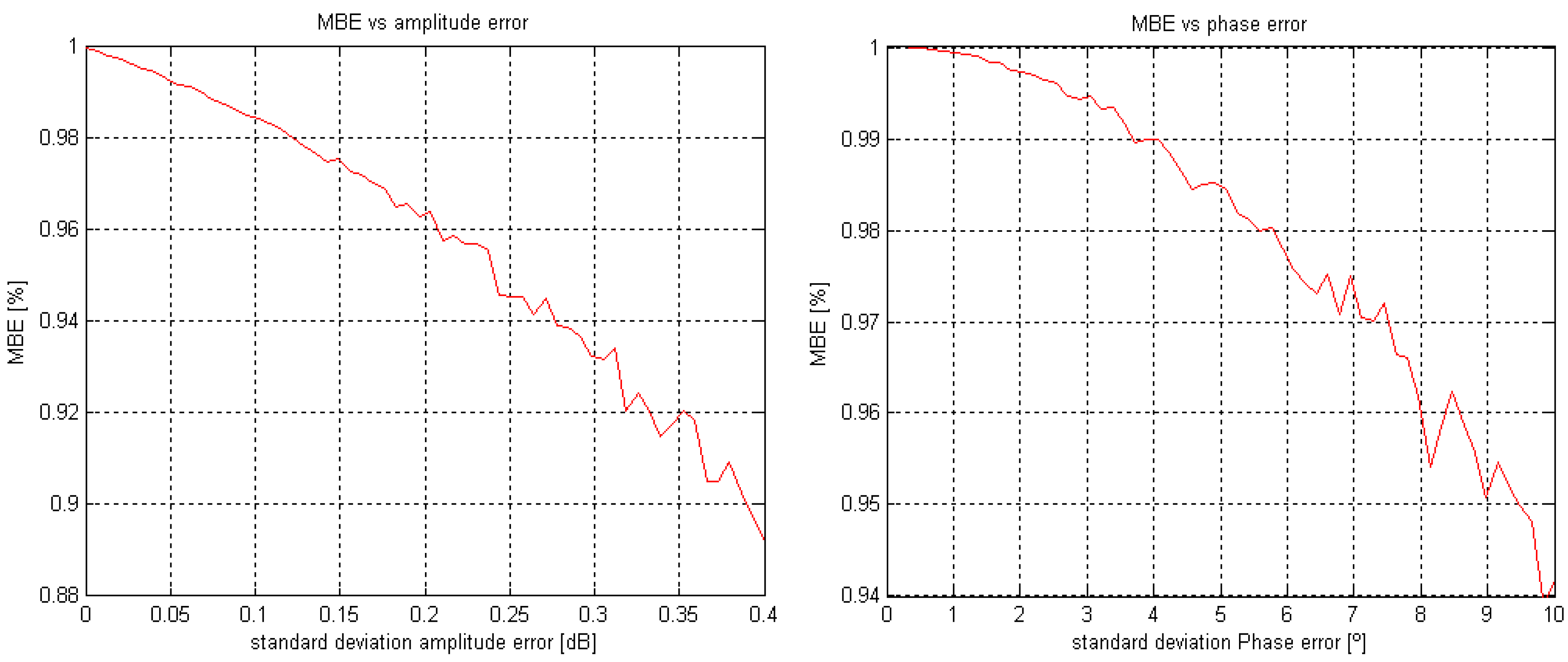
Main Beam Efficiency (MBE) >0.94;

(c)

minimum mutual coupling between the array elements

(d)

cross-pol coupling <−25 dB, and

(e)

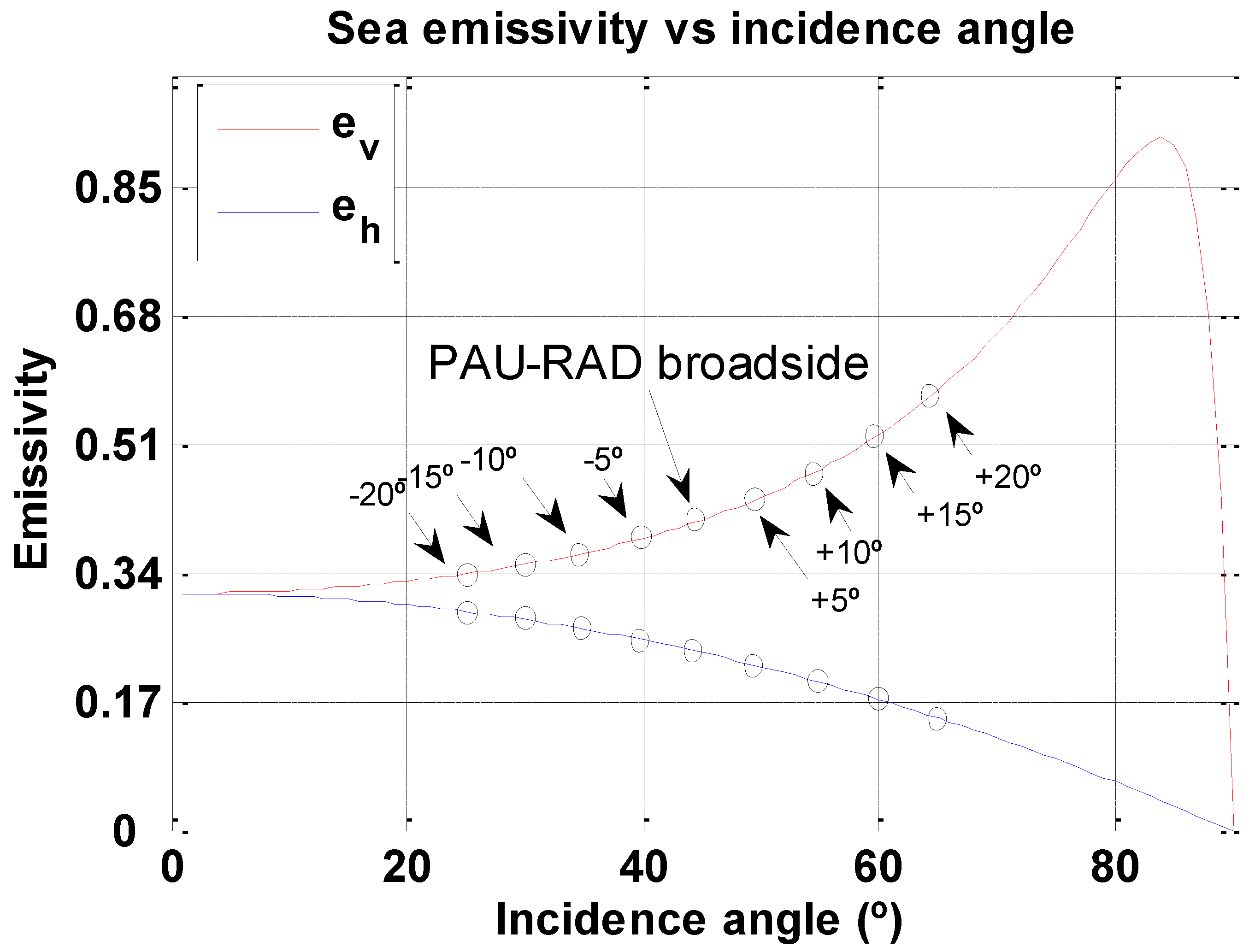
DBF creates the beams in the vertical axis only, with an incidence angle up to ±20° from the array boresight in 5° steps to achieve an angular scan range from 25° to 65° when the antenna is tilted 45° (Figure 1).

A 4 × 4 antenna array with triangular illumination in both directions fulfills these requirements. The orientation of these elementary antennas over the ground plane (Figure 4) takes the antennas feeders into account. For this reason, the elementary antennas have been rotated within adjacent elements to reduce the mutual coupling and the cross-polar component [23,25], and the spacing between array’s elements is 0.63λ (Figure 4).

Figure 4. Polarimetric antenna array for the DBF. Using patch rotated antennas and with a distance between elements of 0.63λ.

Figure 4. Polarimetric antenna array for the DBF. Using patch rotated antennas and with a distance between elements of 0.63λ.

The system requirements specify that it has to be able to steer the beam over the vertical axis direction, so that the antennas are analogically combined in rows (horizontal axis) and the DBF is created in columns (vertical axis).

From here, each antenna is analogically combined with the other three that compose a row (Figure 5) using a RF combiner network with the weights 1:2:2:1 (triangular illumination). Each combiner has its own receiver that down-converts the signal. Finally, the DBF is performed inside the FPGA.

Figure 5. Sketch of the PAU-RAD array antenna configuration. Although the system has digital beamforming capabilities, it has four analog network combiners (with triangular illumination, 1:2:2:1) which compose the horizontal beam and one digital part which performs the digital beam steering on the vertical axis.

Figure 5. Sketch of the PAU-RAD array antenna configuration. Although the system has digital beamforming capabilities, it has four analog network combiners (with triangular illumination, 1:2:2:1) which compose the horizontal beam and one digital part which performs the digital beam steering on the vertical axis.

The above specifications have been set taking into account that PAU-RAD is a ground-based instrument. In this case, the array beamwidth and the beam overlapping do not compromise the geophysical parameters retrieval. In case the system was conceived to be an airborne or spaceborne instrument, some of these parameters have to be improved; for example, the beamwidth would have to be reduced to have an acceptable spatial resolution and non-overlapped beams, which could be achieved with an array larger than 4 × 4.

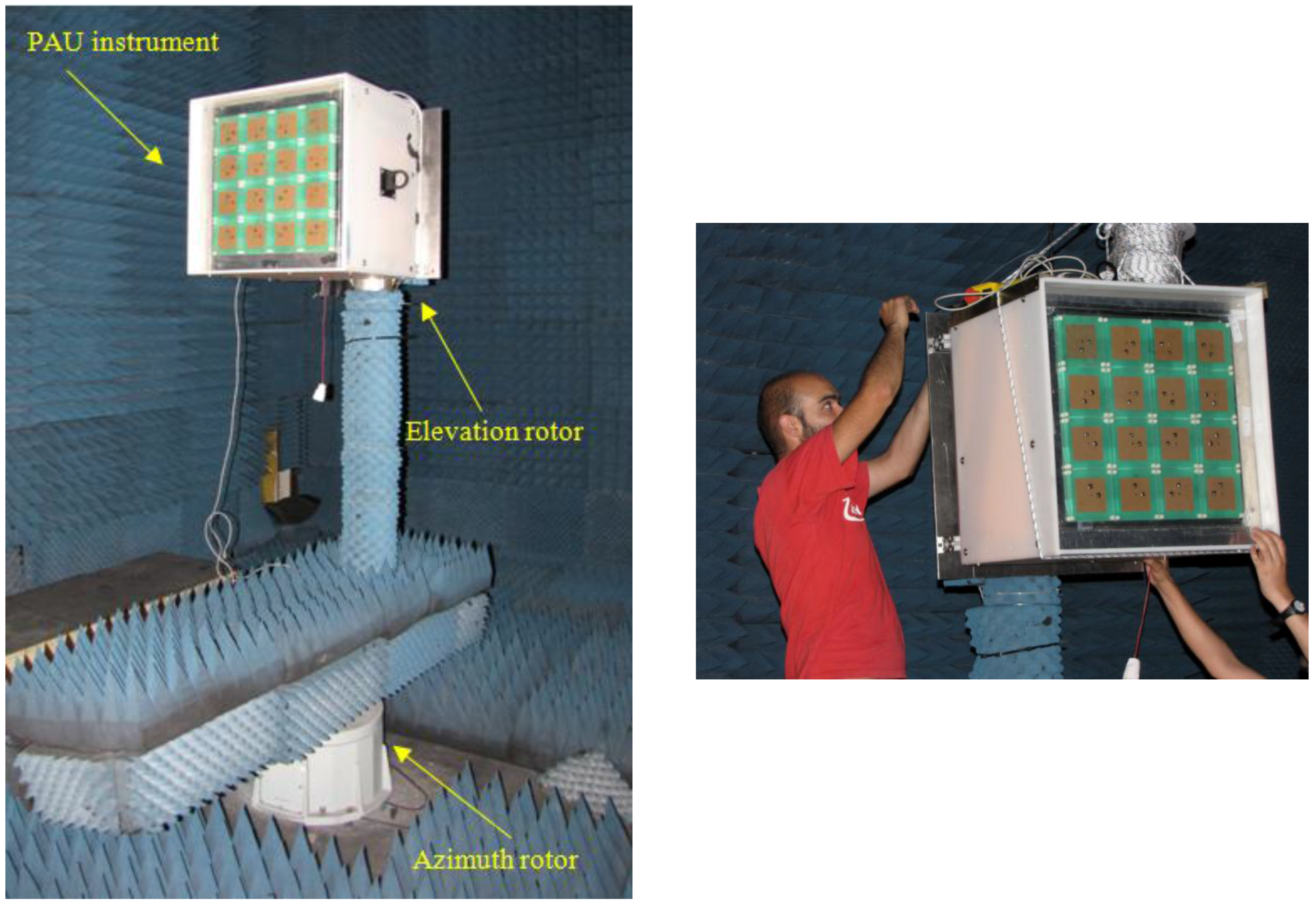
4. PAU-RAD Design, Development and Integration

The PAU instrument (Figure 6 and Figure 7) development has been conducted working in two different packages:

• A hardware package, consisting of the physical instrument and the digital design; and
• a software package, involving all the calibration algorithms, the control unit that manages the digital system, the PC control interface and the data processing algorithms.

Once these two parts are integrated, the instrument is ready to be tested in the anechoic chamber.

Figure 6. Installation of the PAU-RAD instrument on a 110 × 120 × 80 cm structure. On the left side, a frontal perspective with the 4 × 4 element array. On the right side, a back overview with the receivers, the thermal control sub-system and other PAU processors sub‑systems.

Figure 6. Installation of the PAU-RAD instrument on a 110 × 120 × 80 cm structure. On the left side, a frontal perspective with the 4 × 4 element array. On the right side, a back overview with the receivers, the thermal control sub-system and other PAU processors sub‑systems.

Figure 7. PAU sub-systems. (Top left) opened RF-IF dual-polarization receiver with four channels. (Top right) dual-channel ADC sub-system. (Bottom) processor terrace that is placed in the middle of the instrument (Figure 6) and contains the CNS, clock distribution, ADC set, clock reference, clock distribution, and FPGA where the digital hardware and the software algorithms are implemented.

Figure 7. PAU sub-systems. (Top left) opened RF-IF dual-polarization receiver with four channels. (Top right) dual-channel ADC sub-system. (Bottom) processor terrace that is placed in the middle of the instrument (Figure 6) and contains the CNS, clock distribution, ADC set, clock reference, clock distribution, and FPGA where the digital hardware and the software algorithms are implemented.

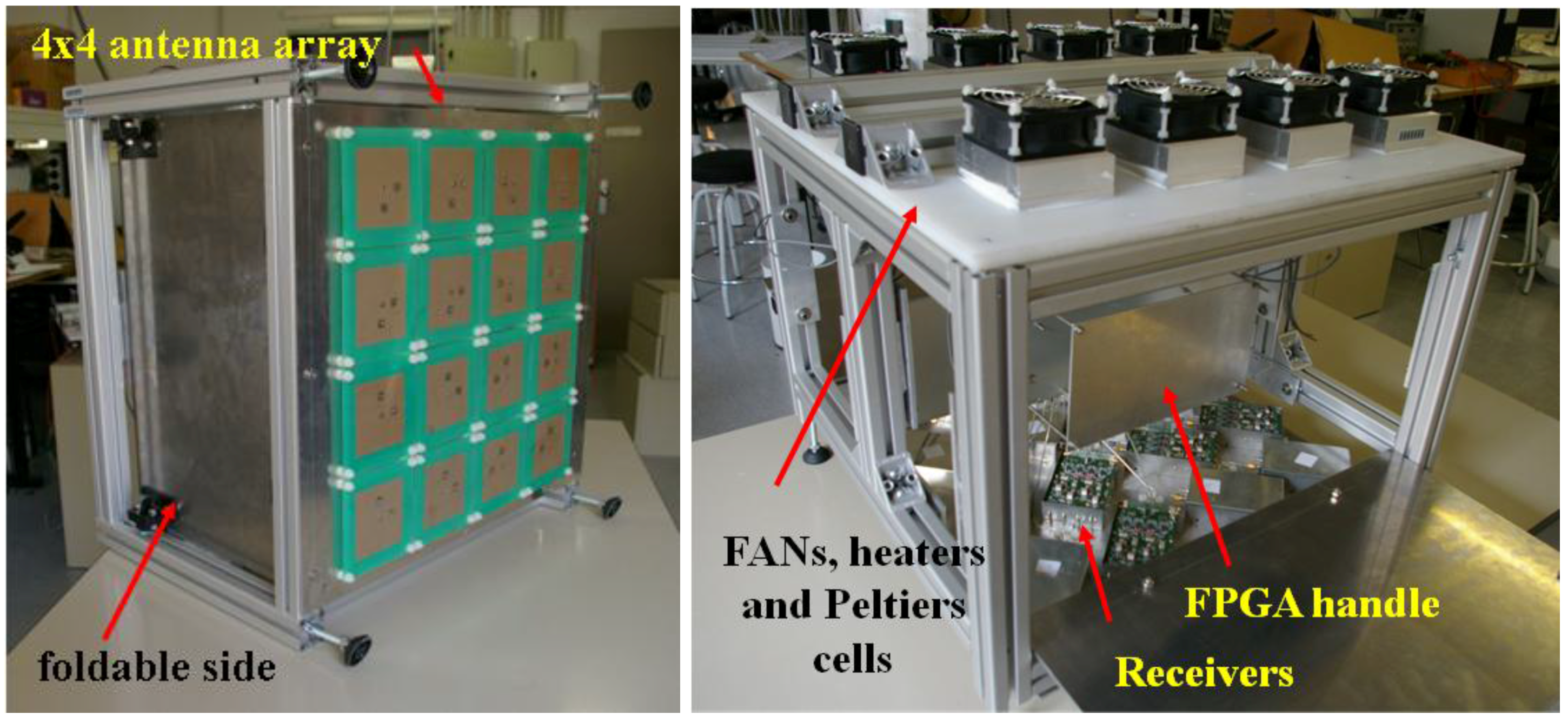
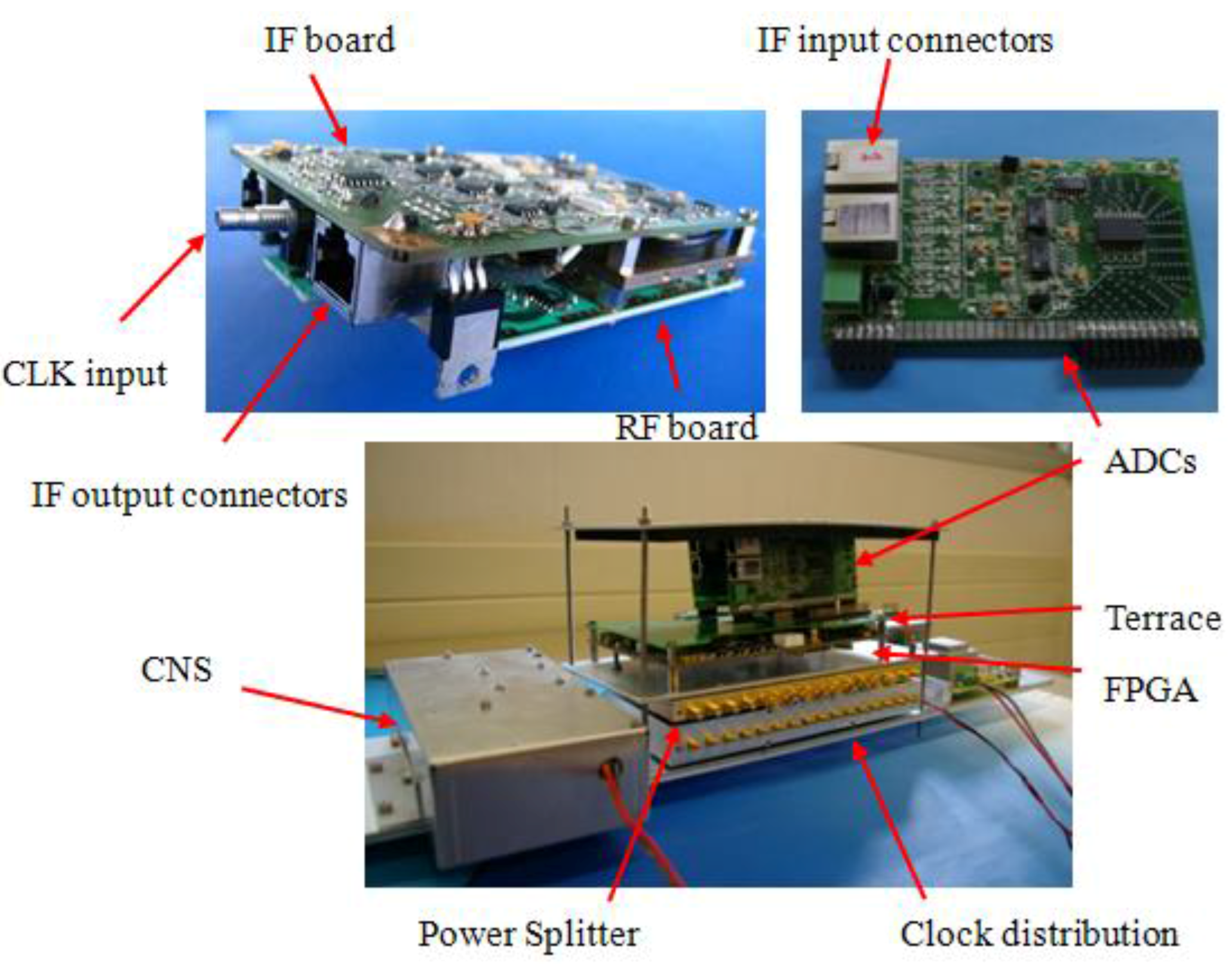
4.1. PAU-RAD Hardware Description

The hardware involves the design of the RF-IF receiver, analog-to-digital converters set [11], digital design and FPGAs, power management and thermal insulation and control. The thermal control part consists of a commercial Proportional Integrative Derivative (PID) control using a 100 Platinum Resistance Thermometer (PT100) sensor, offering an excellent accuracy over a wide temperature range. The control uses an H-bridge to drive enough current to eight 2 A Peltier cells, which are the active part of the control. Each Peltier cell is assembled with fans and heat sinks to ensure an efficient thermal system. PAU-RAD is thermally insulated by using expanded polystyrene foam (EPS) boards, which has a high thermal resistivity [26] of about 28 mK/W. Moreover, internal fans are used to obtain a good temperature homogenization. With this thermal control system, a previously tested demonstrator [11] has achieved an internal temperature variation of ΔT_internal < 0.2 °C.

The radiometer’s core (Figure 8) consists of an analog part, that performs the RF-IF down‑conversion from 1.57542 GHz to 4.039 MHz, and a digital part, that performs the DBF and the correlation radiometer.

The RF-IF receivers (Figure 2) are the most sensitive parts of the analog part and they have been specially designed to avoid channel cross-talk, EMC problems, and to achieve a frequency response of at least 30 dB attenuation in the rejected band (Figure 9).

Figure 8. Analog and digital hardware block diagram. Note that each I/Q down‑conveter has its own Numerical Controlled Oscillator (NCO).

Figure 8. Analog and digital hardware block diagram. Note that each I/Q down‑conveter has its own Numerical Controlled Oscillator (NCO).

Figure 9. Typical frequency response of a RF-IF receiver. The test receiver has been driven with a CW input of −130 dBm at f_GPS-L1 = 1,575.42 MHz. The output is a tone with a −19.52 dBm at f_IF = 4.309 MHz. The rejected-band has a >40 dB of attenuation with respect to the pass-band.

Figure 9. Typical frequency response of a RF-IF receiver. The test receiver has been driven with a CW input of −130 dBm at f_GPS-L1 = 1,575.42 MHz. The output is a tone with a −19.52 dBm at f_IF = 4.309 MHz. The rejected-band has a >40 dB of attenuation with respect to the pass-band.

As discussed in Section 3, the DBF implies strong hardware calibration requirements. The RF front-end was designed with these a priori specifications. Two switches at the RF section of each receiver, allow the selection of the input from three different ports: (a) The antenna signal, for radiometric measurements; (b) the correlated noise signals, for phase and amplitude calibration purposes; and (c) the uncorrelated noise signals, for offset calibration purposes. The antenna signal input is connected directly to the patch antenna, while the uncorrelated noise input is connected to an internal matched load. The most relevant input port is the correlated noise one, which is connected to the CNS (Figure 10) through a 1:16 power splitter for calibration purposes (Section 3.2) for all the system receivers.

Figure 10. Controlled Noise Source (CNS) block diagram. The core of this sub-system is the noise source Noise Com NC346.

Figure 10. Controlled Noise Source (CNS) block diagram. The core of this sub-system is the noise source Noise Com NC346.

The CNS consists of a temperature controlled box with a very stable noise source (NC346, ENR = 17.5 dB at 1.5 GHz, 0.009 dB/K and 0.002 dB/%V), a variable attenuator, and a mechanical switch connected to the variable attenuator and to a matched load. With this hardware configuration (CNS + power splitter) and properly choosing the attenuators, it is possible to have a common signal of 450, 370 or 300 K at the input of each receiver. Receivers’ response is linear within these three values and they are separated enough to ensure a correct performance of the differential calibration (Section 3.2).

Figure 11. ALU–CU-interface PC data flux sketch.

Figure 11. ALU–CU-interface PC data flux sketch.

The digital part, embedded inside the FPGA, has been designed in two parts for simplicity (Figure 11). One part is a self-designed Arithmetic-Logic Unit (ALU), where the DBF and radiometric data process takes place, and a Control Unit (CU), using a NIOS2 from ALTERA [27] (a 32 bit VHDL-embedded microprocessor).

The ALU (Figure 8 and Figure 11) has tree sub-systems:

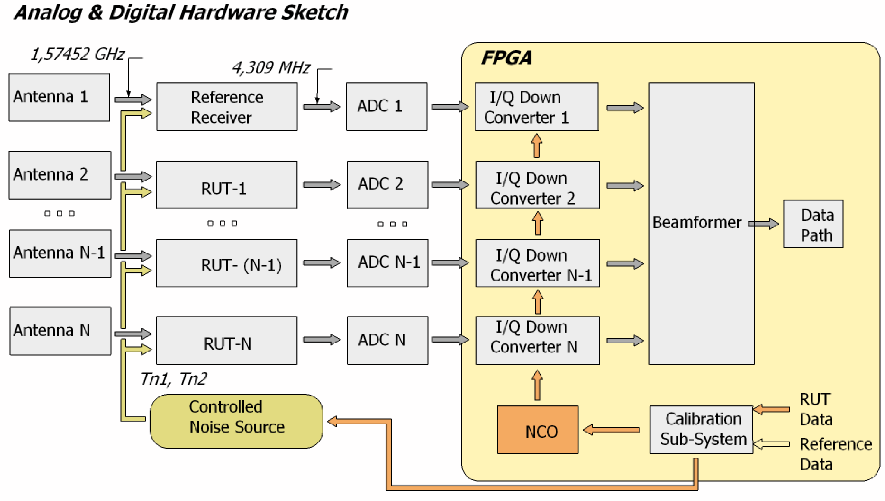
• Correlation radiometer: Once the beam signals are synthesized (one for the upper channel and another for the lower channel), the correlation radiometer part performs the complex correlation between them. The main tasks of this part are the digital down-conversion to the baseband, low-pass filtering the signals, synthesis of the beams, and correlation of the resulting signals to obtain the Stokes parameters.
• Numerically Controlled Oscillators (NCOs): Is a set of oscillators, each channel has its own NCO. In this case, every individual oscillator consists of a simple look-up table accessed periodically and sequentially. The CU updates the NCO’s amplitude and phase according to the requirements. This is a crucial sub-system of the design, since the NCO set not only down‑converts the signals to baseband, but it also calibrates the amplitude and phase errors, and steers the beam for all the receivers. The content of each RUT look-up table is:

  $$Tabl{e}_{RUT}(n)=(A_{Beam}\cdot A_{Cal-RUT}\cdot A_{ph})·\cos \left(2\pi \cdot \Omega \cdot n+({\varphi }_{Beam}-{\varphi }_{Cal-RUT}-{\varphi }_{ph})\right),$$

  (10)

  where:

  • Ω and n are the digital frequency and digital time, respectively;
  • A_Beam and φ_Beam are the modulus and phase of the complex weight, assigned to each RUT to steer the beam in the desired direction;
  • A_Cal-RUT and φ_Cal-RUT are the modulus and phase of the complex weight, assigned to each RUT for hardware calibration purposes; and
  • A_ph and φ_ph are the modulus and phase of the complex weight, to correct any antenna error such as center phase or different path lengths. These values were measured at the UPC anechoic chamber and set as a system parameter.

The sub-system for the hardware error estimation (Figure 12) is an 8 bit complex correlator.

Figure 12. Error estimation and calibration sketch. The ALU performs the complex correlation and the error correction (NCO) and the CU performs the error retrieval and the 1D- Kalman filter.

Figure 12. Error estimation and calibration sketch. The ALU performs the complex correlation and the error correction (NCO) and the CU performs the error retrieval and the 1D- Kalman filter.

The complex correlation between a reference receiver signal and a RUT signal gives information about the amplitude and phase differences among them (Equations (5,6)). Thereafter, this value is sent to the CU, where the mathematical algorithms to derive the amplitude and the phase differences are implemented. This information is used to update the corresponding RUT’s NCO look-up table.

4.2. PAU-RAD Software Description

The software written for PAU-RAD accomplishes the following functions:

• Implements the PAU-RAD finite state machine and the calibration algorithms. This part is running on the CU over a NIOS2 microprocessor, embedded in the FPGA. This software is written in ANSI C language;
• there is a user-friendly control interface on the remote PC side, from where the instrument is operated and the acquired data is stored. This part is written in C# language; and
• the communications channel between the CU and the PC consists of a bidirectional serial communication protocol using a universal asynchronous receiver/transmitter (UART). Over this serial protocol, there is a self-designed application layer, which ensures the communications.

The CU is a finite state machine that changes the system status according to some internal variables (Figure 13). The most important state variables are the integration time for each radiometric sample, and the inter-calibration time between hardware calibrations.

Figure 13. CU finite states machine diagram and interactions.

Figure 13. CU finite states machine diagram and interactions.

The states of the CU can be classified in two sequences: The main sequence that perform the radiometric normal operation, and the validation sequences used for testing. The main sequence states are:

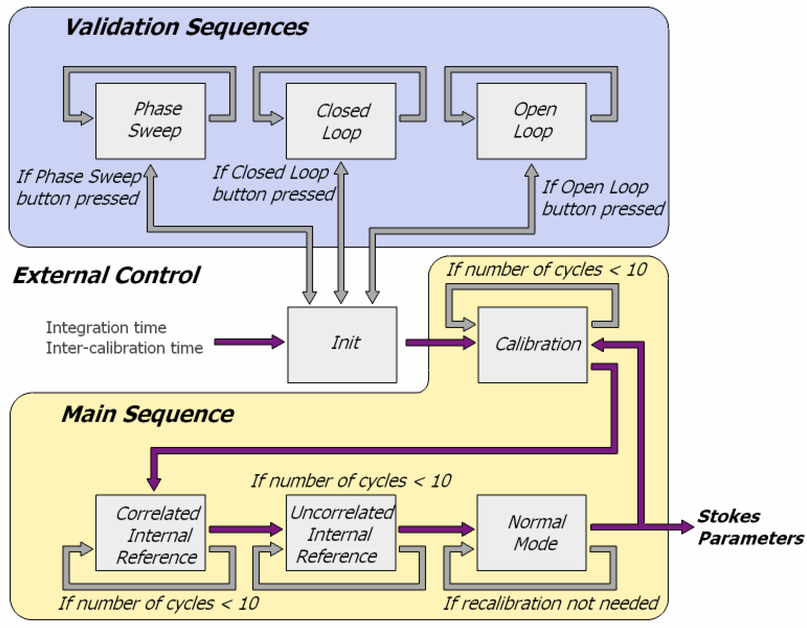
• Init: This is the initialization mode and awaits the PC remote control connection.
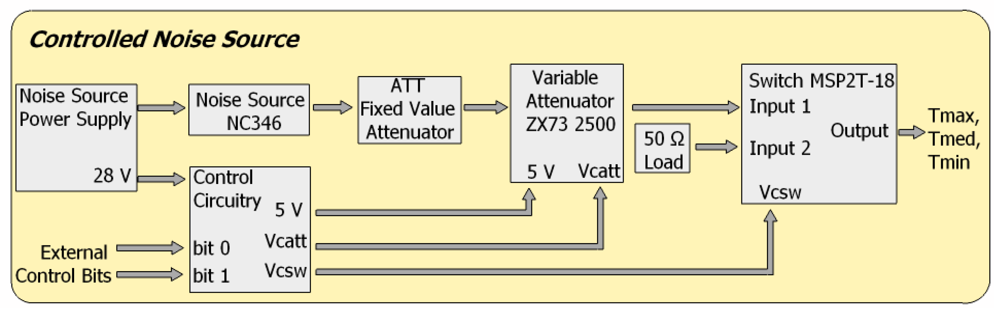
• Calibration: The CU sets the ALU to measure the complex cross-correlations between the reference receiver and, sequentially, the other ones, when the CNS is connected to receivers’ inputs. The input temperature value is selected from the three possible values by the CU with two control bits. The measured amplitude and phase at different time instants are then filtered using a Kalman filter to reduce the noise variance (Section 3.2). Finally, the CU updates RUT’s look-up table following Equation (8) and modifying the NCO amplitude and phase values accordingly. At this time, the relative calibration has been performed and the DBF is ready to operate.
• Correlated Internal Reference: The CU sets the ALU to compute the Stokes parameters from the signals obtained after the DBF, when the CNS is connected to receiver’s inputs. This mode is used to perform the internal radiometric calibration, maximizing the period between external calibrations and is performed for each synthesized beam.
• Uncorrelated Internal Reference: The CU sets the ALU to compute the Stokes parameters from the signal obtained after the DBF, when the matched loads are connected to receivers’ inputs. This mode is used to compute the offsets of the Stokes parameters and it is performed for each synthesized beam.
• Normal mode: The CU sets the ALU to compute the Stokes parameters (radiometric observables) from the signals obtained after the DBF, when the antennas are connected to the receiver’s inputs. The system stays in this mode since the receiver phase and gain drifts degrade the beam. This loop is shown in Figure 12 labeled as if calibration not needed. This period is established empirically and depends on the required performance and application. Moreover, it determines the tradeoff between calibration and measurement time.

The validation sequences states are:

• Phase Sweep: The CU sets the ALU to measure the complex cross-correlations between the reference receiver and a RUT. The goal of this sequence is to sweep the phase of each NCO from 0 to 2π. As described in [28] this test helps to determine amplitude unbalances between I and Q branches, quadrature and phase errors, and offset errors. In PAU-RAD, since signals are sampled at IF and I/Q demodulation and low-pass filtering is performed digitally, there are only offset errors; therefore only information related to the RUT’s complex offset is obtained.
• Open Loop: Same as previous, but with all RUTs and keeping the NCO constant to evaluate RUTs’ temporal drifts.
• Closed Loop: same as previous, but updating the RUTs’ NCO to track calibration errors.

The control interface has the total control of the instrument. The communications between the control interface and the CU is bidirectional. Some of the most relevant applications consist of the possibility to change the integration time, the inter-calibration period, the current CU status, the steering angle of the synthesized beam, among others. Furthermore, the interface has a real-time display to present the information sent by the CU. The most relevant information is displayed with regard to the system status, the current radiometric acquisitions, and RUTs calibration information. The graphical interface helps in understanding the system’s operation and detecting hardware or software errors. All the received data is collected, time stamped and stored for further processing.

5. DBF Performance

In order to test the PAU-RAD performance, the instrument was mounted in an azimuth antenna rotor (Figure 14) at UPC anechoic chamber [29]. After thermal stabilization, the antenna array was illuminated with a noise signal at GPS-L1 frequency transmitted by a corrugated horn.

The tests performed are grouped in three categories:

• Evaluation of the hardware calibration goodness, measuring its impact on the DBF and correction of the array phase center [30] (the point from which the electromagnetic radiation spreads spherically outward, with the phase of the signal being equal at any point on the sphere);
• DBF stability; and
• quality of the beams.

Figure 14. UPC anechoic chamber [29] set up for measuring the PAU-RAD instrument.

Figure 14. UPC anechoic chamber [29] set up for measuring the PAU-RAD instrument.

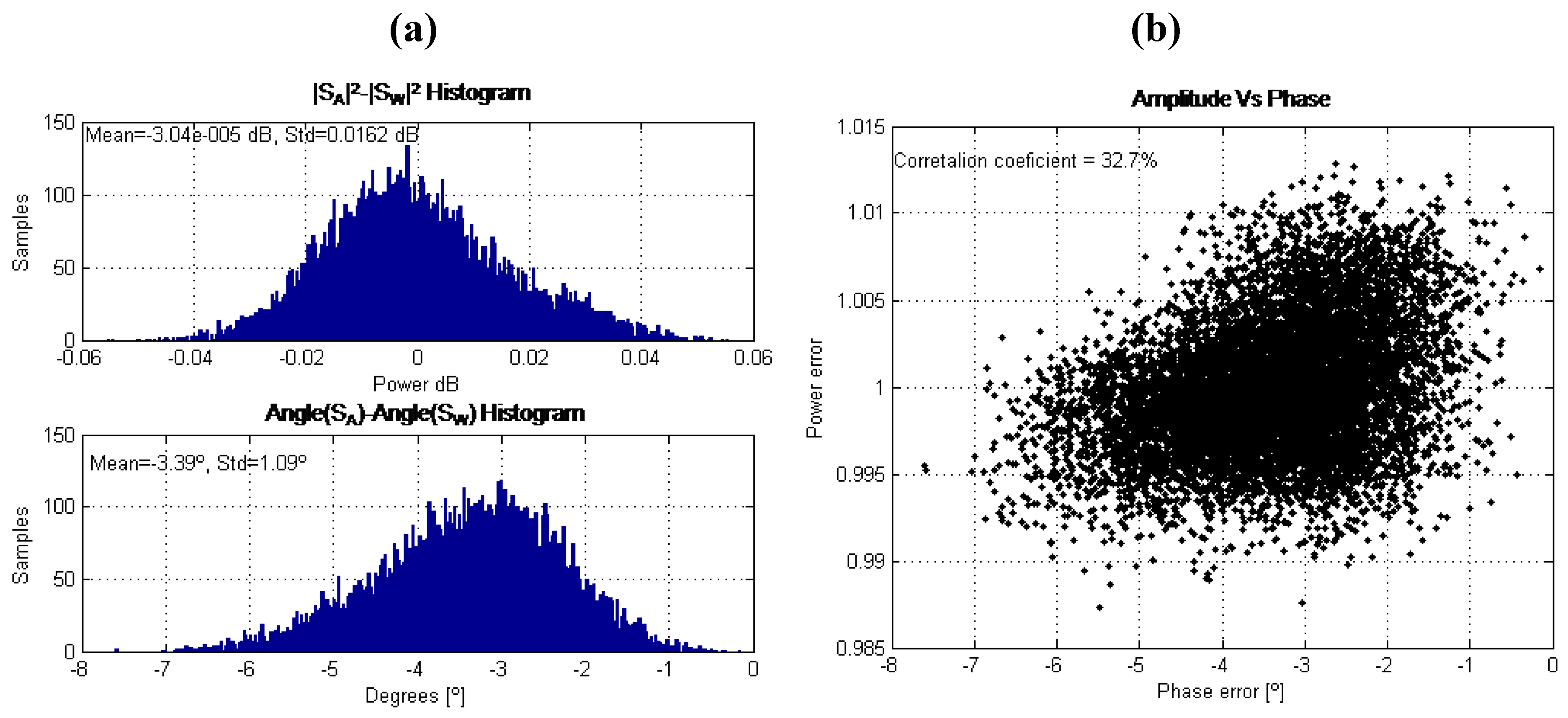
5.1. Evaluation of the Calibration Goodness and Correction of the Phase Center

Receivers have different paths for the signals coming from the CNS and from the antenna (Figure 8). Moreover, this difference changes among receivers, and it has to be empirically measured and further compensated on the calibration algorithms. Furthermore, the correction of the array phase center is still another effect that has to be measured and further compensated on the calibration algorithms. This was the aim of the first test performed in the anechoic chamber. Once the phase and amplitude of the analog receivers have been calibrated, the system was set to measure antenna signal cross-correlations in order to estimate the phase and amplitude error between the CNS and the antenna signal path. Slight corrections among receivers (<4° and <0.2 dB) were required, and it was efficiently solved by adding these measured divergences to the weighting calibration coefficients (A_ph and φ_ph in Equation 9). A miss estimation of these parameters can introduce an offset on the direction of the steered beams and, a loss of performance as well.

5.2. DBF Stability

Once the feasibility of the calibration approach and the DBF performance are checked, the instrument stability is analyzed. For this purpose, the synthesized beam was steered to 0° and radiometric data was acquired during 30 minutes with an integration time of 100 ms.

Figure 15 shows the results of this test. Figure 15(a) shows the amplitude and phase histograms of the synthesized beam; its fluctuations are related to the drifts or error of the unitary receivers. The amplitude’s standard deviation is 0.016 dB and the phase’s standard deviation is 1.09°, well below calibration requirements. Although the standard deviation is well below that of the calibration requirement there is a phase offset (−3.39°) due to the residual error of the CNS-antenna path and phase center calibration.

Figure 15. PAU-RAD DBF results. (a) Synthesized beam stability (fluctuations due to unitary receivers); the standard deviation of the amplitude is 0.0162 dB and of the phase is 1.09°. (b) Synthesized beam correlation between the amplitude and phase error, the plot shows that there is some correlation (32.7%). The data set consists of 30 minutes of data with the beam steering at 0º with no azimuth scan; each sample has an integration time of 100 ms.

Figure 15. PAU-RAD DBF results. (a) Synthesized beam stability (fluctuations due to unitary receivers); the standard deviation of the amplitude is 0.0162 dB and of the phase is 1.09°. (b) Synthesized beam correlation between the amplitude and phase error, the plot shows that there is some correlation (32.7%). The data set consists of 30 minutes of data with the beam steering at 0º with no azimuth scan; each sample has an integration time of 100 ms.

Figure 15(b) shows the scatter plot of the amplitude and phase errors of the beam. The correlation coefficient is low (32.7%), but not zero. This result brings up the question of the dependence between these two parameters, based on their relationship in the NCO originating from the round-off errors due to the finite number of bits.

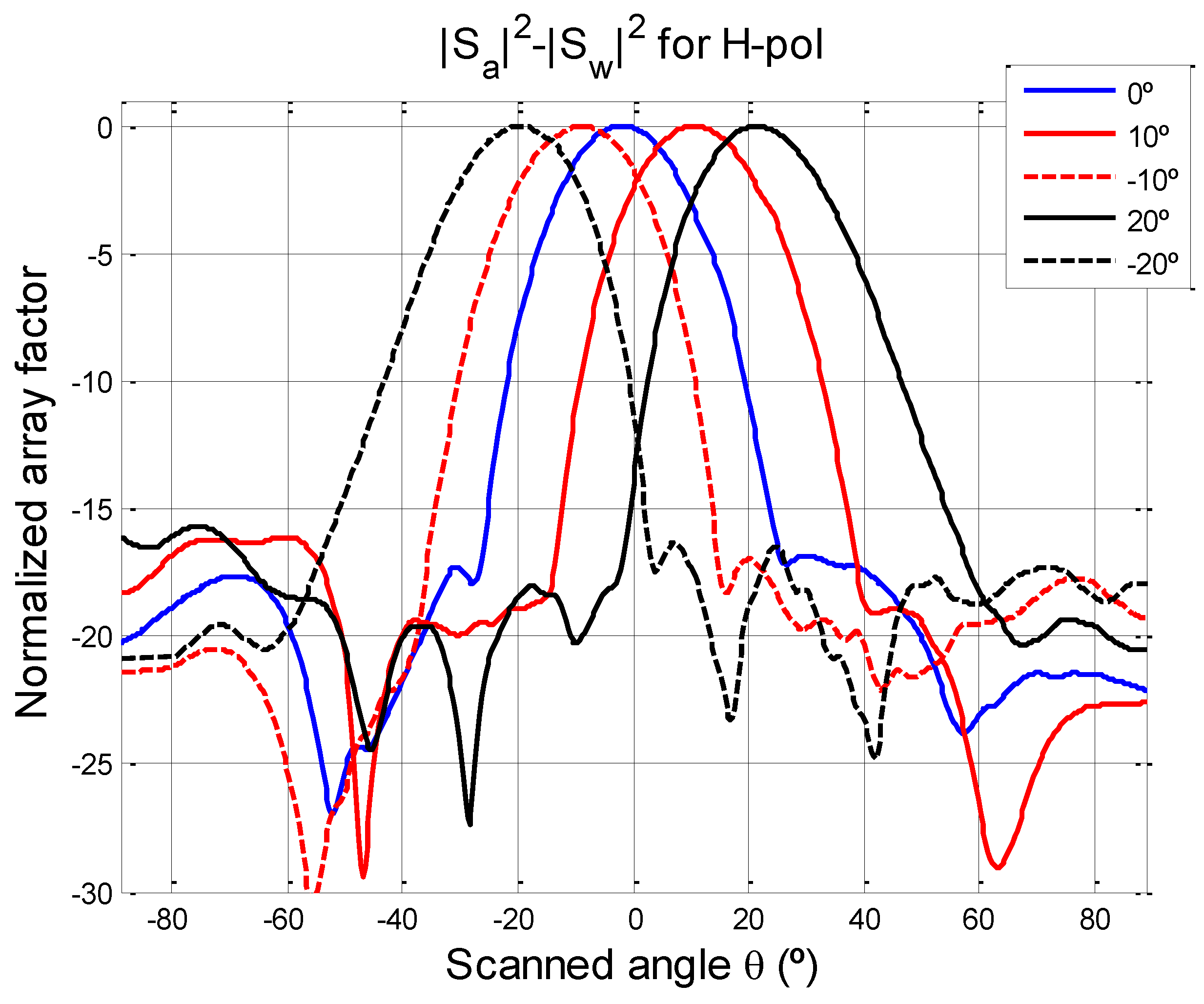
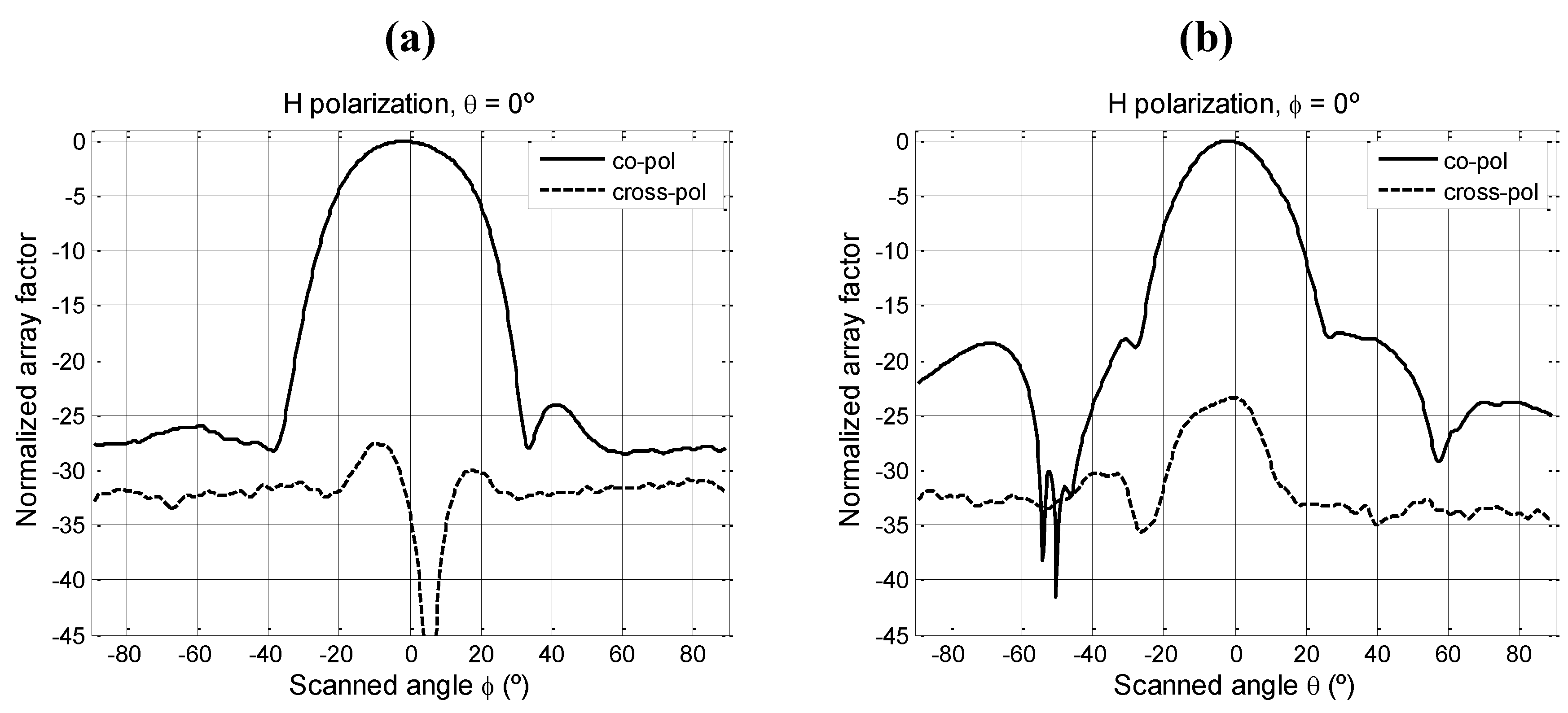
5.3. Beam Synthesis Performance and Steering Tests

The aim of the final test was to study the performance of the beams. As the system is fully polarimetric, the DBF has to be characterized for the four Stoke’s parameters. As the antennas of the system have only two polarizations, vertical and horizontal, the third and fourth parameters are measured by cross-correlating these inputs. The beams of the third and fourth parameters are identical among them because they are the real and imaginary parts, respectively, of the cross-correlation of the horizontal and vertical beams. Then the analysis is focused in the horizontal (H) and vertical (V) polarizations, and the cross-correlation (VH).

To compute the MBE and the beamwidth of beams synthesized in different directions, the whole pattern was measured by scanning across the azimuth angle (φ) range and the elevation angle (θ) range.

The synthesized beam was steered from −20° to +20° in 5° steps, in total nine different beams. For the sake of clarity only five of these normalized DBF results are presented in Figure 16, these beams correspond to the horizontal polarization scanning across the θ angle. Synthesized beams in Figure 16 shows a side lobe level (SLL) [FS2] of −17 dB, in the best case, the 0º steering beam, and a −16 dB in the worse case, for the ±20° angle. Furthermore, in some beams there is a misalignment of ±2° due to the residual calibration error, which does not impact the instrument’s performance.

Figure 16. PAU-RAD DBF results. Measured normalized array factors in dB for multiple beams (H-pol and scanning the θ domain range).

Figure 16. PAU-RAD DBF results. Measured normalized array factors in dB for multiple beams (H-pol and scanning the θ domain range).

Table 1 and Table 2 summarize the results in terms of MBE and beamwidth for the V, H and VH beams. For all the possible steering angles the MBE is better than 91% and the best result is for 0^o where the MBE reaches a value of 95.6% for HV, 94.8% for H and 93.4% for the V polarization. On the other hand, the worst results were, as expected, when the angle of steering is high (±20°). Note that the design specification was to have a MBE higher than 94%, which has been achieved for the 0° steering beam and was almost fulfilled for all steerable beams.

Table 1. MBE for the synthesized beams.

Polarization Beam steering	H	V	HV
−20°	92.5%	91.8%	94.2%
−15°	93.2%	92.6%	95.0%
−10°	93.2%	92.7%	95.1%
−5°	93.3%	92.9%	95.2%
0°	94.8%	93.4%	95.6%
5°	92.9%	92.5%	95.0%
10°	92.8%	91.9%	95.0%
15°	92.7%	91.7%	94.2%
20°	92.3%	91.2%	93.8%

Table 1. MBE for the synthesized beams.

Polarization Beam steering	H	V	HV
−20°	92.5%	91.8%	94.2%
−15°	93.2%	92.6%	95.0%
−10°	93.2%	92.7%	95.1%
−5°	93.3%	92.9%	95.2%
0°	94.8%	93.4%	95.6%
5°	92.9%	92.5%	95.0%
10°	92.8%	91.9%	95.0%
15°	92.7%	91.7%	94.2%
20°	92.3%	91.2%	93.8%

The other design parameter was the beamwidth. In this case the best performance was again for the 0^o steering angle when the Δθ_−3dB = 22.8° for H, Δθ_−3dB = 22.4° for V and Δθ_−3dB = 23.33° for HV. Again, the worst results were for the largest steering angles when the beamwidth values reach the maximum of Δθ_−3dB = 25.5°. TZhe beamwidth requirements were therefore fulfilled in almost all cases. In addition, Table I shows that the HV beams showed the best performance in terms of MBE, but the largest beamwidth. This is due to the way this beam is created from the cross-correlation of the H and V beams.

Table 2. Δθ_−3dB for the synthesized beams.

Polarization Beam steering	H	V	HV
−20°	24.6°	24.2°	24.8°
−15°	25.0°	24.8°	25.5°
−10°	24.1°	24.0°	24.6°
−5°	23.7°	23.1°	24.2°
0°	22.8°	22.4°	23.3°
5°	23.7°	23.3°	24.2°
10°	24.6°	24.2°	24.8°
15°	23.8°	23.5°	24.2°
20°	24.2°	24.1°	24.6°

Table 2. Δθ_−3dB for the synthesized beams.

Polarization Beam steering	H	V	HV
−20°	24.6°	24.2°	24.8°
−15°	25.0°	24.8°	25.5°
−10°	24.1°	24.0°	24.6°
−5°	23.7°	23.1°	24.2°
0°	22.8°	22.4°	23.3°
5°	23.7°	23.3°	24.2°
10°	24.6°	24.2°	24.8°
15°	23.8°	23.5°	24.2°
20°	24.2°	24.1°	24.6°

Once the steering capabilities and excellent performance of the instrument had been demonstrated, Figure 17, Figure 18 and Figure 19 analyze the polarimetric nature of the beams. For brevity purposes only the 0° steering angle has been shown.

Figure 17(a) shows the DBF results in dB for the 0° steered beam and H polarization for the polar and cross-polar beams scanning on the non-steerable domain (φ). In this case the SLL is −25 dB and the cross-polar level is −30 dB, which fulfills another design requirement (<25 dB). Figure 16b shows the steerable beam which is slightly worse than the previous one but still has a good performance. The SLL is −17.5 dB and the cross-polar level is −25 dB.

Figure 17. PAU-RAD DBF results in dB for the 0° steered beam and H polarization, (a) polar and cross-polar beams scanning on the φ domain (non-steerable), (b) polar and cross-polar beams scanning on the θ domain (steerable).

Figure 17. PAU-RAD DBF results in dB for the 0° steered beam and H polarization, (a) polar and cross-polar beams scanning on the φ domain (non-steerable), (b) polar and cross-polar beams scanning on the θ domain (steerable).

Figure 18(a) shows the DBF results in dB for the 0º steered beam and V polarization for the polar and cross-polar beams scanning on the non-steerable domain (φ). In this case, the SLL is −20 dB and the cross-polar level is −27 dB. Figure 18(b) shows the steerable beam which is again slightly worse than the previous one but still has a good performance. The SLL is −17.5 dB and the cross-polar level is −27 dB.

Figure 18. PAU-RAD DBF results in dB for the 0° steered beam and V polarization, (a) polar and cross-polar beams scanning on the φ domain (non-steerable), (b) polar and cross-polar beams scanning on the θ domain (steerable).

Figure 18. PAU-RAD DBF results in dB for the 0° steered beam and V polarization, (a) polar and cross-polar beams scanning on the φ domain (non-steerable), (b) polar and cross-polar beams scanning on the θ domain (steerable).

Figure 19 shows the θ = 0° and φ = 0° cuts of the HV polarization. This case is different from the two previous cases, because the third Stokes parameter is collected through the real part of this antenna pattern product and the fourth one from the imaginary part. So that, amplitude and phase of the cross-correlation beam have to be presented to show the instrument performance in this full polarimetric mode. Figure 19(a,c) shows the modulus in dB of the DBF results for the 0° steered beam and HV polarization for the φ and θ domains, respectively. In both cases, the SLL is better than −22.5 dB. Figure 19(b,d) shows the phase of the DBF results for the 0° steered beam and HV polarization, at the main beam there is a phase error of 1.5°, which induces an error of about −17 dB in the fourth and third parameters.

Figure 19. PAU-RAD DBF results in dB for the 0° steered beam and HV polarization, (a) modulus of the beam scanning on the φ domain (non-steerable); (b) phase of the beam on the φ domain; (c) modulus of the beam scanning on the θ domain (steerable); (d) phase of the beam scanning on the θ domain (steerable).

Figure 19. PAU-RAD DBF results in dB for the 0° steered beam and HV polarization, (a) modulus of the beam scanning on the φ domain (non-steerable); (b) phase of the beam on the φ domain; (c) modulus of the beam scanning on the θ domain (steerable); (d) phase of the beam scanning on the θ domain (steerable).

6. Conclusions and Ongoing Work

A digital beamforming radiometer has been completely developed. This achievement includes the hardware, calibration algorithms, and control software. A comprehensive set of tests have been carried out to understand the capabilities of the instrument: Simultaneous multi-angular measurements can be obtained, and the hardware calibration is satisfactory provided. Receivers’ amplitude and phase can be equalized by using a NCO, which is also used to steer the DBF. System stability allows inter‑calibration periods to be longer than 30 minutes. First results of the DBF have been presented for the vertical, horizontal and the correlation polarization, fulfilling the design requirements and satisfactorily showing the capabilities of this new instrument and its synthesized beams.

Next steps will be the preparation of the instrument for ocean and land measurements.

References

1. Barre, H.M.J.; Duesmann, B.; Kerr, Y.H. SMOS: The mission and the system. IEEE Trans. Geosci. Remote Sens. 2008, 46, 587–593. [Google Scholar] [CrossRef]
2. Le Vine, D.M.; Lagerloef, G.S.E.; Colomb, F.R.; Yueh, S.H.; Pellerano, F.A. Aquarius: An instrument to Monitor Sea Surface Salinity from Space. IEEE Trans. Geosci. Remote Sens. 2007, 47, 2040–2050. [Google Scholar] [CrossRef]
3. Swift, C.; McIntosh, R.E. Considerations for microwave remote sensing of ocean surface salinity. IEEE Trans. Geosci. Remote Sens. 1983, 21, 480–491. [Google Scholar] [CrossRef]
4. Marquardt, D. An algorithm for least-squares estimation of non-linear parameters. J. Soc. Indust. Appl. Math. 1963, 11, 431–441. [Google Scholar] [CrossRef]
5. Talone, M.; Camps, A.; Gabarro, C.; Sabia, R.; Gourrion, J.; Vall-llossera, M.; Mourre, B.; Font, J. Contributions to the Improvement of the SMOS Level 2 Retrieval Algorithm: Optimization of the Cost Function. In Proceedings of 2008 IEEE International Geoscience & Remote Sensing Symposium, Boston, MA, USA, July 6–11, 2008; Volume 4, pp. 943–937.
6. Gabarro, C.; Font, J.; Miller, J.; Camps, A.; Burrage, D.; Wesson, J. Use of empirical sea surface emissivity models for a rough estimation of sea surface salinity from an airborne microwave radiometer. Scientia Marina 2008, 72, 329–336. [Google Scholar]
7. Camps, A.; Font, J.; Vall-llossera, M.; Corbella, I.; Duffo, N.; Torres, F.; Blanch, S.; Aguasca, A.; Villarino, R.; Gabarro, C.; Enrique, L.; Miranda, J.; Sabia, R.; Talone, M. Determination of the sea surface emissivity at L-band and its applications to SMOS salinity retrieval algorithms: Review of the contributions of the UPC–ICM. Radio Sci. 2008, 43, RS3008. [Google Scholar] [CrossRef]
8. Camps, A.; Vall-llossera, M.; Corbella, I.; Duffo, N.; Torres, F. Improved image reconstruction algorithms for Aperture Synthesis Radiometers. IEEE Trans. Geosci. Remote Sens. 2008, 46, 146–158. [Google Scholar] [CrossRef]
9. Ramos-Perez, I.; Bosch-Lluis, X.; Camps, A.; Valencia, E.; Marchan-Hernandez, J.F.; Rodriguez-Alvarez, N.; Canales-Contador, F. Preliminary Results of the Passive Advanced Unit Synthetic Aperture (PAU-SA). In Proceedings of 2009 IEEE International Geoscience & Remote Sensing Symposium, Cape Town, South Africa, July 12–17, 2009; Volume 4, pp. 121–124.
10. Camps, A.; Bosch-Lluis, X.; Ramos-Perez, I.; Marchan-Hernandez, J.F.; Izquierdo, B.; Rodriguez, N. New instrument concepts for ocean sensing: Analysis of the PAU-Radiometer. IEEE Trans. Geosci. Remote Sens. 2007, 45, 3180–3192. [Google Scholar] [CrossRef]
11. Bosch-Lluis, X.; Camps, A.; Ramos-Perez, I.; Marchan-Hernandez, J.F.; Rodriguez-Alvarez, N.; Valencia, E. PAU/RAD: Design and preliminary calibration results of a new L-Band pseudo-correlation radiometer concept. Sensors 2008, 8, 4392–4412. [Google Scholar] [CrossRef]
12. Marchan-Hernandez, J.F. Sea State Determination Using GNSS-R Techniques: Contributions to the PAU Instrument. Ph. D. Thesis, Universitat Politècnica de Catalunya, Barcelona, Spain, 2009. [Google Scholar]
13. Marchan-Hernandez, J.F.; Camps, A.; Rodriguez-Alvarez, N.; Bosch-Lluis, X.; Ramos-Perez, I.; Valencia, E. PAU/GNSS-R: Implementation, performance and first results of a real-time Delay-Doppler map reflectometer using global navigation satellite system signals. In Sensors; 2008; Volume 8, pp. 3005–3018. [Google Scholar]
14. Valencia, E.; Marchan-Hernandez, J.F.; Camps, A.; Rodriguez-Alvarez, N.; Tarongi, J.M.; Piles, M.; Ramos-Perez, I.; Bosch-Lluis, X.; Vall-llossera, M.; Ferre, P. Experimental Relationship between the Sea Brightness Temperature Changes and the GNSS-R Delay-Doppler Maps: Preliminary Results of the Albatross Field Experiments. In Proceedings of 2009 IEEE International Geoscience & Remote Sensing Symposium, Cape Town, South Africa, July 12–17, 2009; Volume 3, pp. 741–744.
15. Rodriguez-Alvarez, N.; Camps, A.; Bosch-Lluis, X.; Ramos-Perez, I.; Marchan-Hernandez, J.F. Sea Surface Temperature Retrieval Using IR-Radiometry and Atmospheric Modeling: Simulation and Experimental Results Using PAU-IR. In Proceedings of 2007 IEEE International Geoscience & Remote Sensing Symposium, Barcelona, Spain, July 23–28, 2007; 2007; pp. 933–936. [Google Scholar]
16. Randa, J.; Lahtinen, J.; Camps, A.; Gasiewski, A.J.; Hallikainen, M.; Le Vine, D.M.; Martin-Neira, M.; Piepmeier, J.; Rosenkranz, P.W.; Ruf, C.S.; Shiue, J.; Skou, N. Recommended Terminology for Microwave Radiometry; NIST Technical Note TN1551; National Institute of Standards and Technology: Gaithersburg, MD, USA, 2008. [Google Scholar]
17. Bosch-Lluis, X.; Ramos-Perez, I.; Camps, A.; Rodriguez-Alvarez, N.; Marchan-Hernandez, J.F.; Valencia, E. Digital Beamforming Analysis and Performance for a Digital L-Band Pseudo-Correlation Radiometer. In Proceedings of 2009 IEEE International Geoscience & Remote Sensing Symposium, Cape Town, South Africa, July 12–17, 2009; Volume 5, pp. 184–187.
18. IEEE Standard VHDL Synthesis Packages. IEEE Standard 1076.3-1997.
19. GPS Receiver RF Front End; GP2015; Zarlink: Ottawa, ON, Canada, September 2007; Available online: http://www.zarlink.com/zarlink/gp2015-datasheet-sept2007.pdf (accessed on December 30, 2010).
20. Camps, A.; Rodriguez-Alvarez, N.; Bosch-Lluis, X.; Marchan-Hernandez, J.F.; Ramos-Perez, I.; Segarra, M.; Sagues, L.; Tarrago, D.; Cunado, O.; Vilaseca, R.; Tomas, A.; Mas, J.; Guillamon, J. PAU in SeoSAT: A proposed hybrid L-band microwave radiometer/GPS reflectometer to improve Sea Surface Salinity estimates from space. In Proceedings of Microwave Radiometry and Remote Sensing of the Environment, Firenze, Italy, March 11–14, 2008; pp. 1–4.
21. Smith, N.; Lefebvre, M. The Global Ocean Data Assimilation Experiment (GODAE). In Proceedings of International Symposium Monitoring Oceans in the 2000s: An Integrated Approach, Biarritz, France, October 15–17, 1997.
22. Sonmez, M.K.; Trew, R.J.; Hearn, C.P. Front-End Topologies for Phased Array Radiometry. In Proceedings of 22nd European Microwave Conference, Helsinki, Finland, September 5–9, 1992; Volume 2, pp. 1251–1256.
23. Villarino, R.M. Empirical Determination of the Sea Surface Emissivity at L-band: A contribution to ESA’s SMOS Earth Explorer Mission. Ph.D. Dissertation, Universitat Politècnica de Catalunya, Barcelona, Spain, 2004. [Google Scholar]
24. Kalman, R.E. A new approach to linear filtering and prediction problems. Trans. ASME–J. Basic Eng.Series D 1960, 82, 35–45. [Google Scholar] [CrossRef]
25. Camps, A.; Font, J.; Vall-llossera, M.; Gabarro, C.; Corbella, I.; Duffo, N.; Torres, F.; Blanch, S.; Aguasca, A.; Villarino, R.; Enrique, L.; Miranda, J.J.; Arenas, R.; Julia, A.; Etcheto, J.; Caselles, V.; Weill, A.; Boutin, J.; Contardo, S.; Niclos, R.; Rivas, R.; Reising, S.C.; Wursteisen, P.; Berger, M.; Martin-Neira, M. The WISE 2000 and 2001 field experiments in support of the SMOS mission: Sea surface L-band brightness temperature observations and their application to sea surface salinity retrieval. IEEE Trans. Geosci. Remote Sens. 2004, 42, 804–823. [Google Scholar] [CrossRef]
26. Standard for the Preparation of Test Procedures for the Thermal Evaluation of Solid Electrical Insulating Materials. IEEE Standard 98-2002, 2002.
27. NIOS II Processor Reference Handbook; ALTERA: San Jose, CA, USA, 2009.
28. Camps, A.; Torres, F.; Corbella, I.; Bara, J.; Soler, X. Calibration and experimental results of a two-dimensional interferometric radiometer laboratory prototype. Radio Sci. 1997, 32, 1821–1832. [Google Scholar] [CrossRef]
29. TSC-UPC Anechoic Chamber. Available online: http://www.tsc.upc.es/researcheef/antennas/antennalab_website/r_grups_amp.html (accessed on December 30, 2010).
30. Nagelberg, E. Fresnel region phase centers of circular aperture antennas. IEEE Trans. Antennas Propagat. 1965, 13, 479–480. [Google Scholar] [CrossRef]