Applicability of the Thermal Infrared Spectral Region for the Prediction of Soil Properties Across Semi-Arid Agricultural Landscapes


 ,
,  , and
, and
Abstract
:1. Introduction
2. Methods
2.1. Soil Sampling and Sample Analyses
2.2. Soil Spectral Measurements
2.2.1. TIR-Emission FTIR Spectroscopy
2.2.2. VNIR-SWIR-Bidirectional Measurements
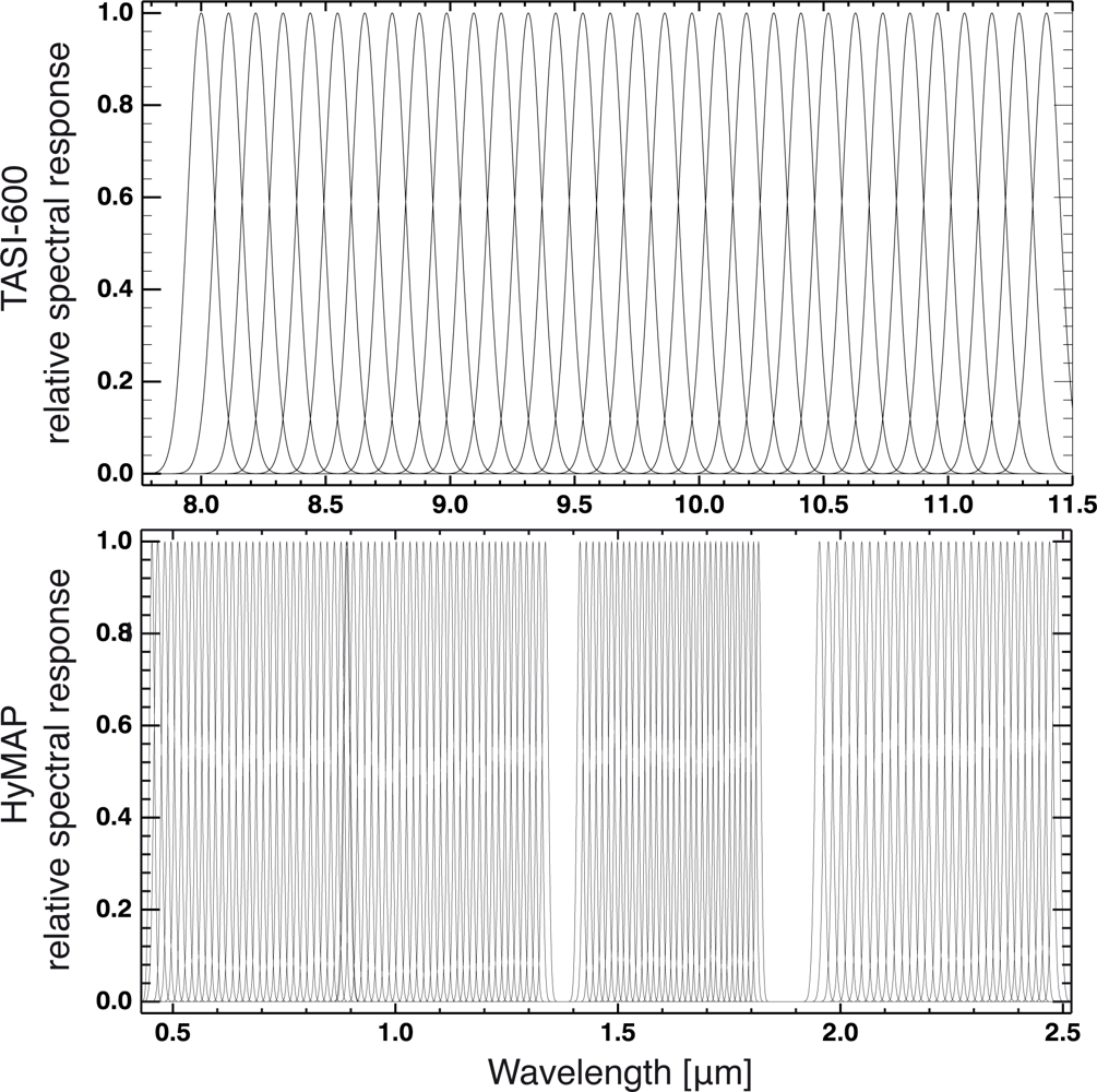
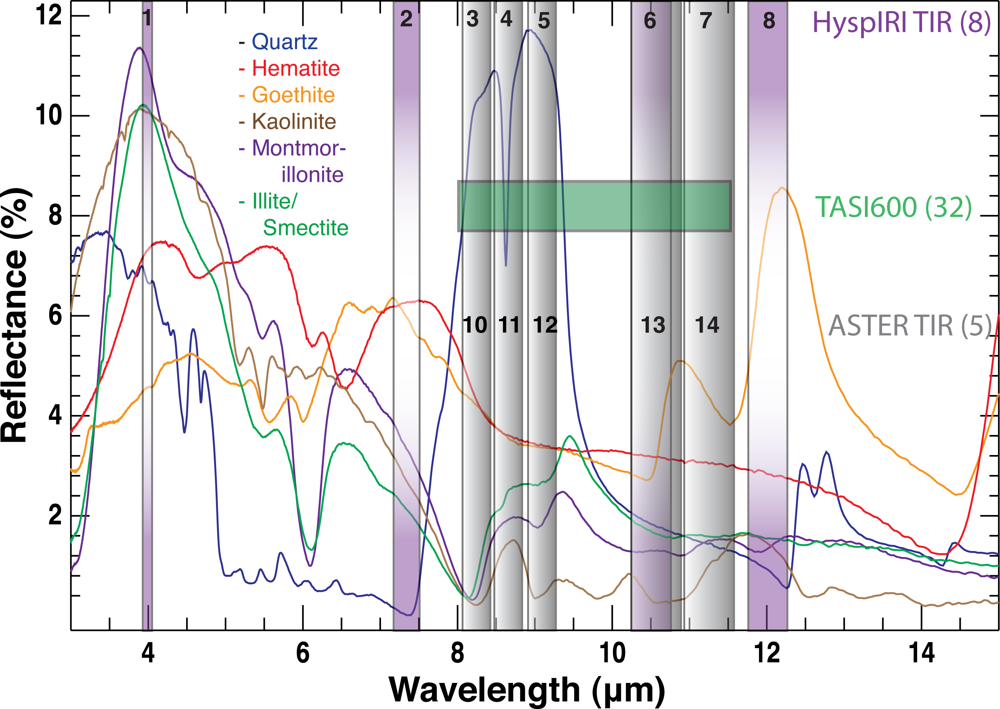
2.2.3. Spectral Resampling to Operational Hyperspectral Remote Sensors
2.3. Multivariate Regression Modelling
2.3.1. PLSR-Calibration and Validation
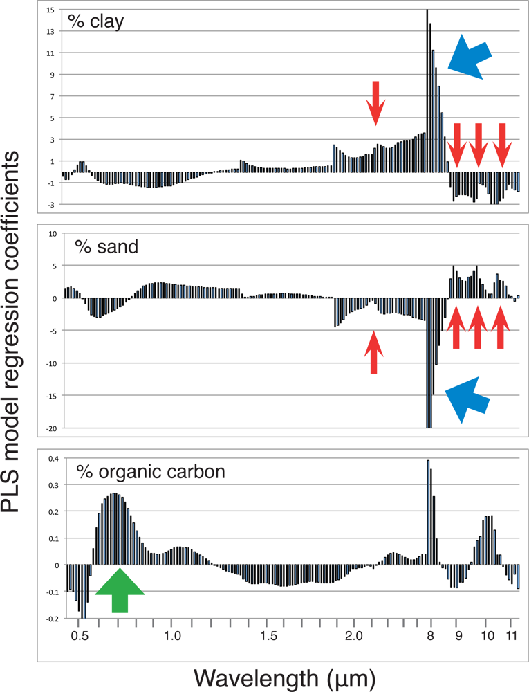
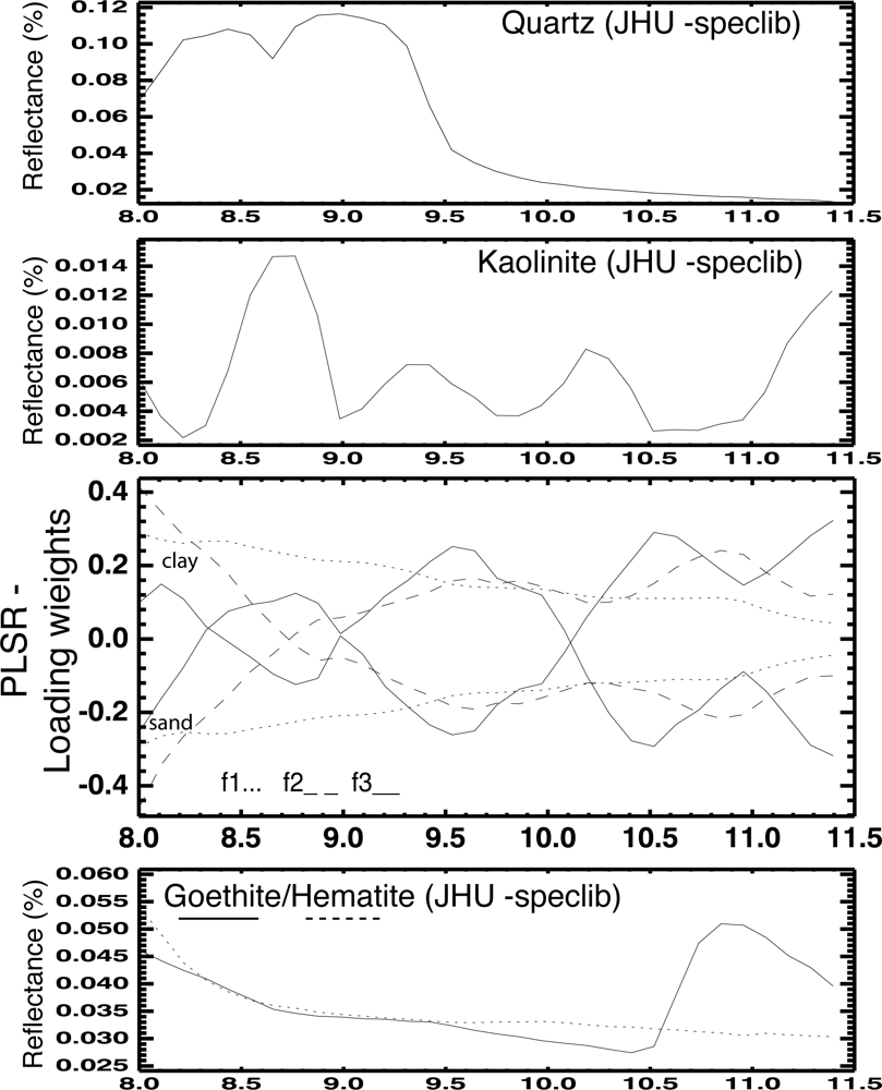
2.3.2. Spectral Interpretation of the PLSR Models
3. Results
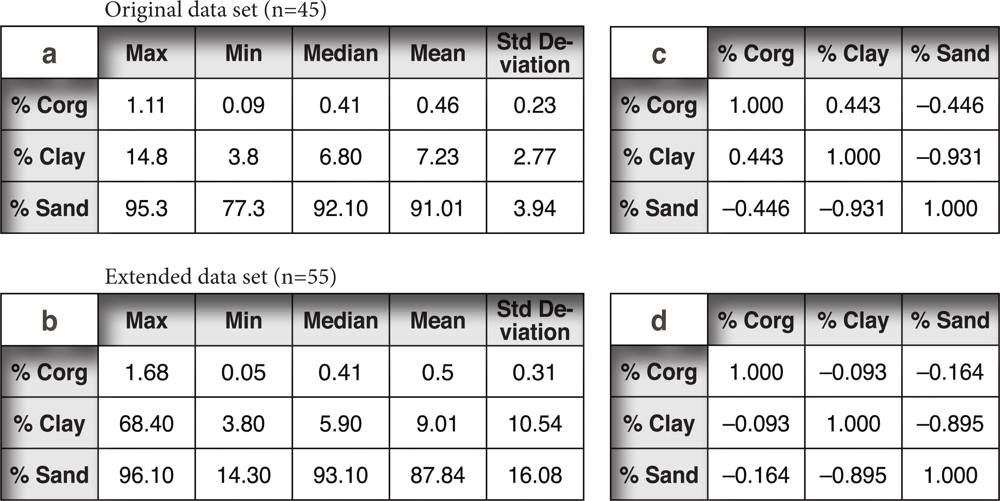
3.1. Soil Analyses
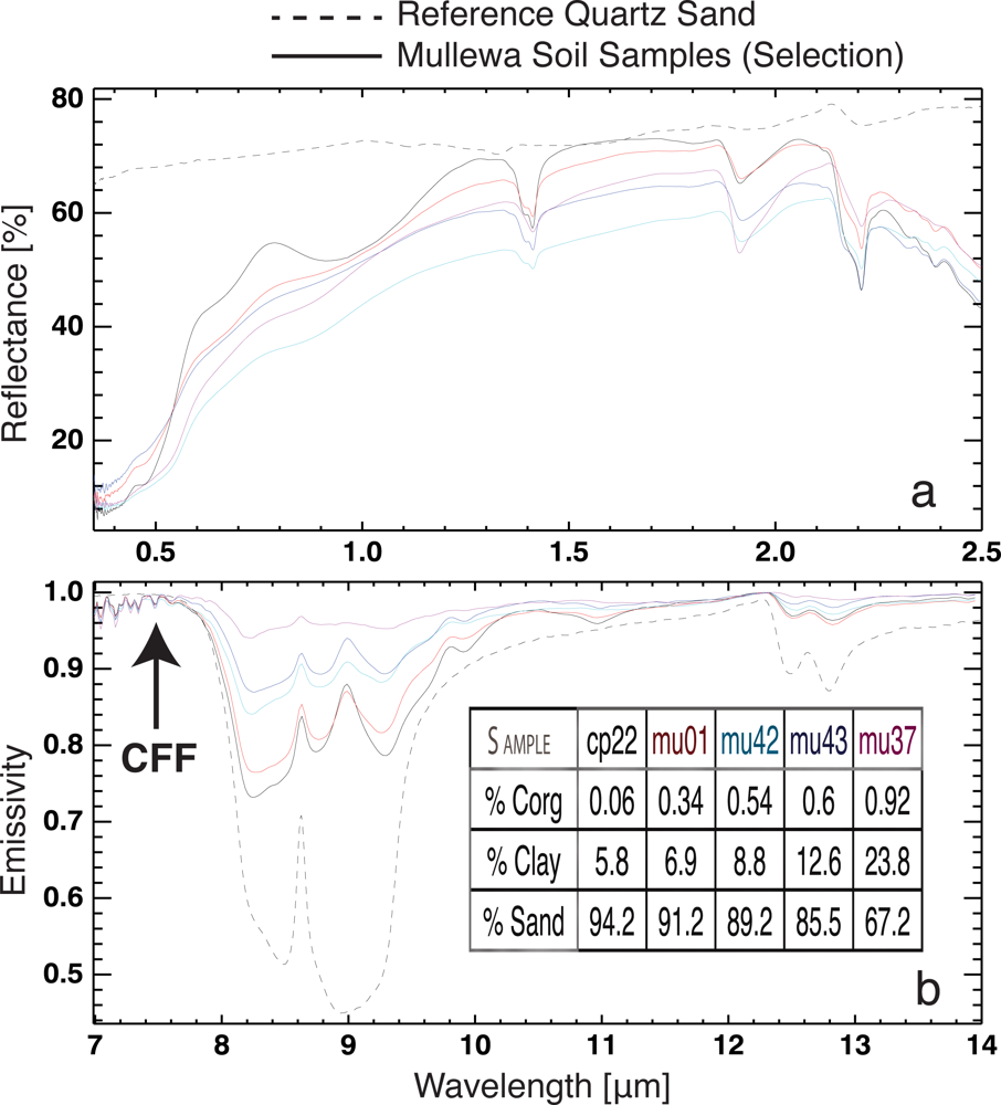
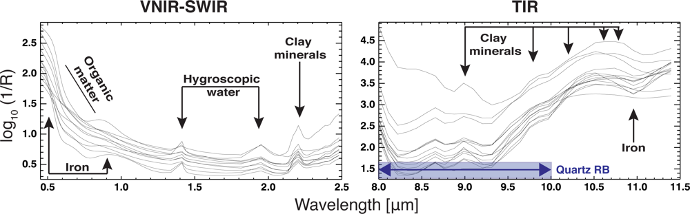
3.2. Soil Spectral Characteristics
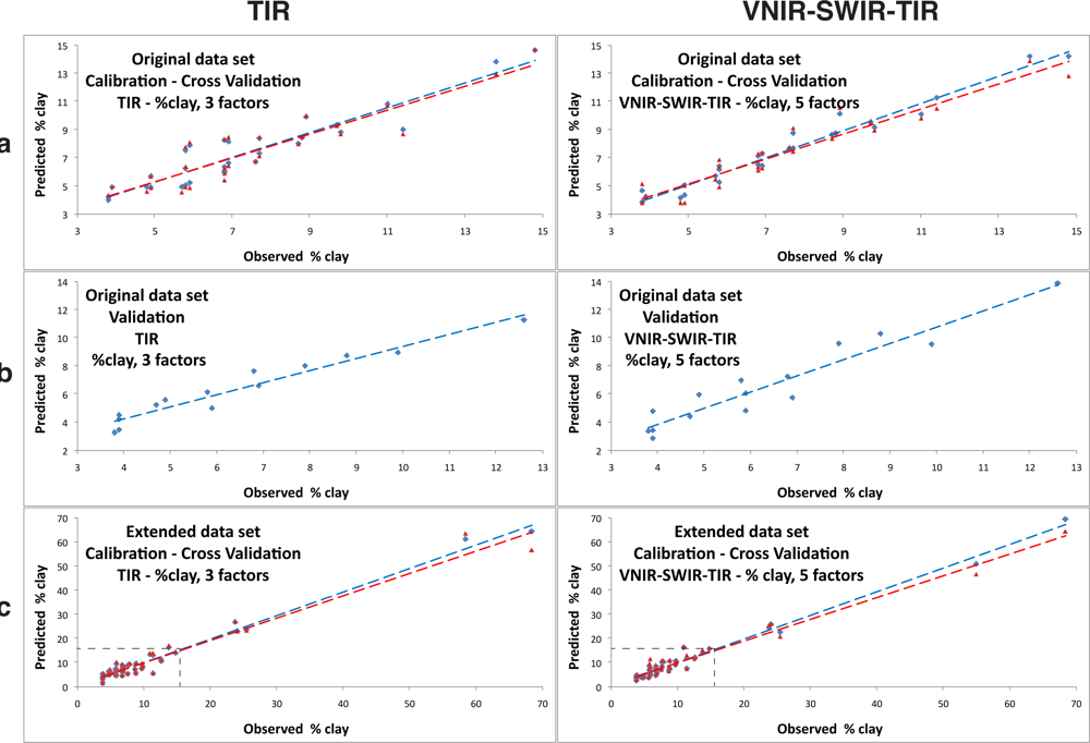
3.3. Prediction of Soil Properties
3.3.1. Clay Content
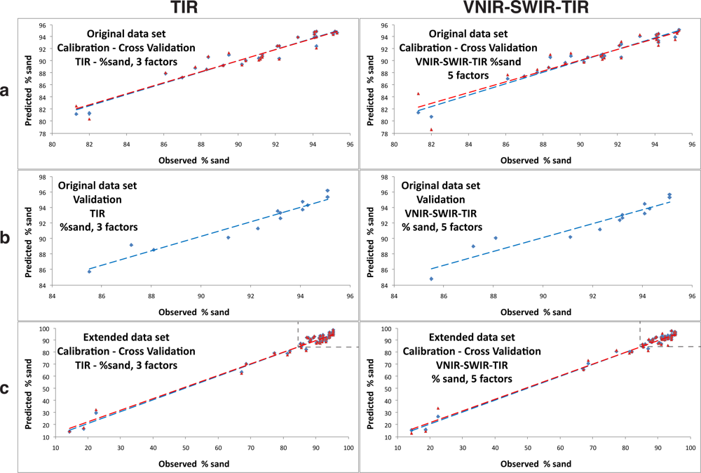
3.3.2. Sand Content
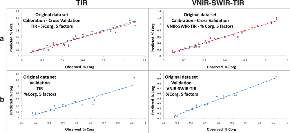
3.3.3. Organic Carbon Content
3.3.4. Spectral Interpretation of the PLSR Models Drivers
4. Discussion
4.1. Extended Data Set
4.2. Silt Fraction
5. Conclusions
Acknowledgments
References
- Ben-Dor, E.; Irons, J.R.; Epema, G. Soil Reflectance. In Remote Sensing for the Earth Sciences: Manual of Remote Sensing; Rencz, A.N., Ed.; John Wiley & Sons, Inc: Hoboken, NJ, USA, 1999; Volume 3, pp. 111–188. [Google Scholar]
- Bartholomeus, H.; Epema, G.; Schaepman, M. Determining iron content in Mediterranean soils in partly vegetated areas, using spectral reflectance and imaging spectroscopy. Int. J. Appl. Earth Obs. Geoinf 2007, 9, 194–203. [Google Scholar] [Green Version]
- Viscarra-Rossel, R.A.; Walvoort, D.; McBratney, A.; Janik, L.; Skjemstad, J. Visible, near infrared, mid infrared or combined diffuse reflectance spectroscopy for simultaneous assessment of various soil properties. Geoderma 2006, 131, 59–75. [Google Scholar]
- Chabrillat, S.; Goetz, A.; Krosley, L.; Olsen, H. Use of hyperspectral images in the identification and mapping of expansive clay soils and the role of spatial resolution. Remote Sens. Environ 2002, 82, 431–445. [Google Scholar]
- Chang, C.; Laird, D. Near-Infrared reflectance spectroscopic analysis of soil C and N. Soil Sci 2002, 167, 110–116. [Google Scholar]
- Ben-Dor, E.; Taylor, R.; Hill, J.; Dematte, J.A.M.; Whiting, M.; Chabrillat, S.; Sommer, S. Imaging spectrometry for soil applications. Adv. Agron 2008, 97, 321–392. [Google Scholar]
- Salisbury, J.W.; Walter, L.; Vergo, N.; D’Aria, D. Infrared (2.1–25 μm) Spectra of Minerals; The Johns Hopkins University Press: Baltimore, MD, USA, 1991. [Google Scholar]
- Salisbury, J.W.; D’Aria, D. Emissivity of terrestrial materials in the 8–14 μm atmospheric window. Remote Sens. Environ 1992, 42, 83–106. [Google Scholar]
- Stenberg, B.; Viscarra-Rossel, R.A. Diffuse Reflectance Spectroscopy for High-Resolution Soil Sensing. In Proximal Soil Sensing, Progress in Soils Science; Viscarra-Rossel, R.A., McBratney, A.B., Minasney, B., Eds.; Springer: Dordrecht, The Netherlands, 2010; pp. 29–47. [Google Scholar]
- Rodgers, A.; Cudahy, T.J. Vegetation corrected continuum depths at 2.20 μm: An approach for hyperspectral sensors. Remote Sens. Environ 2009, 113, 2243–2257. [Google Scholar]
- King, P.; Ramsey, M.; McMillan, P.; Swayze, G. Laboratory Fourier Transform Infrared Spectroscopy Methods for Geologic Samples. In Infrared Spectroscopy in Geochemistry, Exploration Geochemistry and Remote Sensing; King, P.L., Ramsey, M.S., McMillan, P.F., Swayze, G.A., Eds.; Mineralogical Association of Canada: Quebec, QC, Canada, 2004; pp. 57–91. [Google Scholar]
- Hecker, C.; van der Meijde, M.; van der Meer, F. Thermal infrared spectroscopy on feldspars—Successes, limitations and their implications for remote sensing. Earth-Sci. Rev 2010, 103, 60–70. [Google Scholar]
- Martens, H.; Naes, T. Multivariate Calibration; John Wiley & Sons: Hoboken, NJ, USA, 1992. [Google Scholar]
- Esbensen, K.H. Multivariate Data Analysis in Practice: An Introduction to Multivariate Data Analysis and Experimental Design, 5 ed; Camo: Oslo, Norway, 2006. [Google Scholar]
- Rogers, L. Geraldton Region: Land Resources Survey. In Land Resources Series; Wilson, G., Ed.; Departement of Agriculture and Food Western Australia: Perth, WA, Australia, 1996. [Google Scholar]
- Janik, L.; Skjemstad, J.O.; Raven, M. Characterization and analysis of soils using mid infrared partial least-squares. I. Correlations with XRF-determined major-element composition. Aust. J. Soil Res 1995, 33, 621–636. [Google Scholar]
- Janik, L.; Merry, R.; Skjemstad, J. Can mid infra-red diffuse reflectance analysis replace soil extractions? Aust. J. Exp. Agric 1998, 38, 681–696. [Google Scholar]
- McCarty, G.; Reeves, J.B., III; Reeves, V.; Follett, R.; Kimble, J. Mid-infrared and near-infrared diffuse reflectance spectroscopy for soil carbon measurement. Soil Sci. Soc. Am. J 2002, 66, 640–646. [Google Scholar]
- Isbell, R. The Australian Soil Classification; CSIRO Publishing: Melbourne, VIC, Australia, 1996. [Google Scholar]
- McKenzie, N.; Henderson, B.; McDonald, W. Monitoring Soil Change. Principles and Practice for Australian Conditions; Technical Report 18/02; CSIRO Land and Water: Canberra, Australia, 2002. [Google Scholar]
- Walkley, A.; Black, I. An estimation of the Degtjareff method for determining soil organic matter and a proposed modification of the chromic acid titration method. Soil Sci 1934, 37, 29–37. [Google Scholar]
- Salisbury, J.W.; Wald, A.; D’Aria, D. Thermal-infrared remote sensing and Kirchhoff’s law: 1. Laboratory measurements. J. Geophys. Res. 1994. [Google Scholar] [CrossRef]
- Horton, K.A.; Johnson, J.R.; Lucey, P.G. Infrared measurements of pristine and disturbed soils 2. Environmental effects and field data reduction. Remote Sens. Environ 1998, 64, 47–52. [Google Scholar]
- Hook, S.J.; Kahle, A.B. The Micro Fourier Transform Interferometer (mFTIR)—A new fieldspectrometer for aquisition of infrared data of natural surfaces. Remote Sens. Environ 1996, 56, 172–181. [Google Scholar]
- Korb, A.R.; Dybwad, P.; Wadsworth, W.; Salisbury, J.W. Portable Fourier transform infrared spectroradiometer for field measurements of radiance and emissivity. Appl. Opt 1996, 35, 1679–1692. [Google Scholar]
- Nicodemus, F.E. Directional reflectance and emissivity of an opaque surface. Appl. Opt 1965, 4, 767–773. [Google Scholar]
- Salisbury, J.W. Spectral Measurements Field Guide; Technical Report ADA362372; Defense Technology Information Center: Fort Belvoir, VA, USA, 1998. [Google Scholar]
- Kessler, W. Multivariate Datenanalyse für die Pharma-, Bio- und Prozessanalytik; Wiley-VCH: Weinheim, Germany, 2006. [Google Scholar]
- McKenzie, N.; Jacquier, D.; Isbell, R.; Brown, K. Australian Soils and Landscapes; Csiro Publishing: Melbourne, VIC, Australia, 2004. [Google Scholar]
- Salisbury, J.W.; Hapke, B.; Eastes, J. Usefulness of weak bands in midinfrared remote sensing of particulate planetary surfaces. J. Geophys. Res 1987, 92, 702–710. [Google Scholar]
- Baldridge, A.M.; Hook, S.J.; Grove, C.I.; Rivera, G. The ASTER spectral library Version 2.0. Remote Sens. Environ 2009, 113, 711–715. [Google Scholar]
- Lyon, R. Effects of Weathering, Desert-Varnish, etc., on Spectral Signatures of Mafic, Ultramafic and Felsic Rocks, Leonora, West Australia, with Comments on Their Surface Coatings. Proceedings of the Fifth Australian Remote Sensing Conference, Perth, WA, Australia, 8–12 October 1990; pp. 915–923.
- Rivard, B.; Petroy, S.; Miller, J. Measured effects of desert varnish on the mid-infrared spectra of weathered rocks as an aid to TIMS imagery interpretation. IEEE Trans. Geosci. Remote Sens 1993, 31, 284–291. [Google Scholar]
- Wald, A.; Salisbury, J.W. Thermal infrared directional emissivity of powdered quartz. J. Geophys. Res 1995, 100, 24665–24675. [Google Scholar]
- Salisbury, J.W.; Wald, A. The role of volume scattering in reducing spectral contrast of reststrahlen bands in spectra of powdered minerals. Icarus 1992, 96, 121–128. [Google Scholar]
- Ben-Dor, E.; Inbar, Y.; Chen, Y. The reflectance spectra of organic matter in the visible near-infrared and short wave infrared region (400–2,500 nm) during a controlled decomposition process. Remote Sens. Environ 1997, 61, 1–15. [Google Scholar]
- Hunt, G.R.; Salisbury, J.W.; Lenhoff, C. Visible and near-infrared spectra of minerals and rocks: III. Oxides and hydroxides. Modern Geol 1971, 2, 195–205. [Google Scholar]


| Y | Spectral range (bands) | Original Data Set | Extended Data Set | |||||||||
|---|---|---|---|---|---|---|---|---|---|---|---|---|
| f | Cross-VALIDATION | VALIDATION (test data set) | f | Cross-VALIDATION | ||||||||
| n | R2 | RMSEP | n | R2 | RMSEP | n | R2 | RMSEP | ||||
| % clay | VNIR-SWIR (125) | 5 | 29 | 0.9 | 0.94 % | 14 | 0.89 | 0.81 % | 5 | 54 | 0.92 | 2.93 % |
| TIR (32) | 3 | 30 | 0.85 | 1.09 % | 15 | 0.93 | 0.66 % | 3 | 55 | 0.95 | 2.55 % | |
| VNIR-SWIR-TIR (157) | 5 | 28 | 0.93 | 0.85 % | 15 | 0.84 | 0.98 % | 5 | 55 | 0.97 | 2.26 % | |
| % sand | VNIR-SWIR (125) | 6 | 29 | 0.45 | 2.56 % | n.p. | n.p. | n.p. | 5 | 55 | 0.9 | 5.56 % |
| TIR (32) | 3 | 29 | 0.92 | 1.08 % | 13 | 0.93 | 0.82 % | 3 | 55 | 0.97 | 2.73 % | |
| VNIR-SWIR-TIR (157) | 5 | 30 | 0.88 | 1.31 % | 13 | 0.9 | 0.97 % | 5 | 55 | 0.97 | 2.84 % | |
| % Corg | VNIR-SWIR (125) | 7 | 30 | 0.86 | 0.08 % | 15 | 0.81 | 0.06 % | 6 | 54 | 0.73 | 0.14 % |
| TIR (32) | 5 | 30 | 0.91 | 0.08 % | 15 | 0.62 | 0.12 % | 6 | 52 | 0.67 | 0.15 % | |
| VNIR-SWIR-TIR (157) | 5 | 30 | 0.96 | 0.06 % | 15 | 0.95 | 0.04 % | 6 | 52 | 0.8 | 0.11 % | |
Share and Cite
Eisele, A.; Lau, I.; Hewson, R.; Carter, D.; Wheaton, B.; Ong, C.; Cudahy, T.J.; Chabrillat, S.; Kaufmann, H. Applicability of the Thermal Infrared Spectral Region for the Prediction of Soil Properties Across Semi-Arid Agricultural Landscapes. Remote Sens. 2012, 4, 3265-3286. https://doi.org/10.3390/rs4113265
Eisele A, Lau I, Hewson R, Carter D, Wheaton B, Ong C, Cudahy TJ, Chabrillat S, Kaufmann H. Applicability of the Thermal Infrared Spectral Region for the Prediction of Soil Properties Across Semi-Arid Agricultural Landscapes. Remote Sensing. 2012; 4(11):3265-3286. https://doi.org/10.3390/rs4113265
Chicago/Turabian StyleEisele, Andreas, Ian Lau, Robert Hewson, Dan Carter, Buddy Wheaton, Cindy Ong, Thomas John Cudahy, Sabine Chabrillat, and Hermann Kaufmann. 2012. "Applicability of the Thermal Infrared Spectral Region for the Prediction of Soil Properties Across Semi-Arid Agricultural Landscapes" Remote Sensing 4, no. 11: 3265-3286. https://doi.org/10.3390/rs4113265