Satellite-Derived Photic Depth on the Great Barrier Reef: Spatio-Temporal Patterns of Water Clarity

Abstract

Detecting changes to the transparency of the water column is critical for understanding the responses of marine organisms, such as corals, to light availability. Long-term patterns in water transparency determine geographical and depth distributions, while acute reductions cause short-term stress, potentially mortality and may increase the organisms’ vulnerability to other environmental stressors. Here, we investigated the optimal, operational algorithm for light attenuation through the water column across the scale of the Great Barrier Reef (GBR), Australia. We implemented and tested a quasi-analytical algorithm to determine the photic depth in GBR waters and matched regional Secchi depth (Z_SD) data to MODIS-Aqua (2002–2010) and SeaWiFS (1997–2010) satellite data. The results of the in situ Z_SD/satellite data matchup showed a simple bias offset between the in situ and satellite retrievals. Using a Type II linear regression of log-transformed satellite and in situ data, we estimated Z_SD and implemented the validated Z_SD algorithm to generate a decadal satellite time series (2002–2012) for the GBR. Water clarity varied significantly in space and time. Seasonal effects were distinct, with lower values during the austral summer, most likely due to river runoff and increased vertical mixing, and a decline in water clarity between 2008–2012, reflecting a prevailing La Niña weather pattern. The decline in water clarity was most pronounced in the inshore area, where a significant decrease in mean inner shelf Z_SD of 2.1 m (from 8.3 m to 6.2 m) occurred over the decade. Empirical Orthogonal Function Analysis determined the dominance of Mode 1 (51.3%), with the greatest variation in water clarity along the mid-shelf, reflecting the strong influence of oceanic intrusions on the spatio-temporal patterns of water clarity. The newly developed photic depth product has many potential applications for the GBR from water quality monitoring to analyses of ecosystem responses to changes in water clarity.

1. Introduction

The quantification of environmental variables in space and time is essential to understand the ecology of marine organisms and their responses to a changing environment. For benthic organisms, temperature, salinity and the availability of light and nutrients are key parameters controlling their distribution and productivity. Ocean color satellites, such as the NASA Sea-viewing Wide Field-of-view Sensor (SeaWiFS) and the NASA Moderate Imaging Spectroradiometer onboard Aqua (MODIS-Aqua), provide oceanographic data records on spatial and temporal scales unattainable using conventional in situ sampling schemes. The current state of operational satellite remote sensing is that algorithms for measuring geophysical parameters, such as chlorophyll concentration or water clarity, are reasonably reliable over deep water, but still limited in optically shallow regions. Considerable progress has, however, been made in the application of polar orbiting satellite data to mapping nearshore optical properties [1–3]. Recent progress in remote sensing applications includes the development of bio-optical algorithms for determining the photic depth (Z_%; units of m) from the observed satellite radiances. Z_% is a measure of water clarity [4] with, for example, Z_1% reflecting the depth where only 1% of the surface irradiance (PAR, photosynthetic available radiation; units of μE·cm²·s⁻¹) remains. The value of 1% of surface PAR has been conveniently considered as an ecologically important threshold, the “euphotic depth”, or lower limit of the euphotic zone, or “compensation depth”, a depth below which most photo-autotrophic organisms cannot achieve positive net daily production [5,6]. The euphotic depth relates inversely to light attenuation and, thus, provides a direct, intuitive measure of the clarity or transparency of the overlying water column [5].

Detecting changes to the transparency of the water column is critical for understanding the responses of benthic organisms to light availability, especially in shallow coastal and shelf regions, such as the Great Barrier Reef (GBR), Australia [7,8]. Degradation in the condition of coastal and inshore ecosystems due to poor water quality is a key issue for the GBR [9], as terrestrial runoff of excess nutrients and sediments affects turbidity and sedimentation regimes and intermittently increases water column productivity, in turn leading to the deterioration of inshore coral reefs at local scales [10]. Water clarity is considered a key measure of water quality on the GBR, with Secchi depth (Z_SD; units of m) being the most widely used measure. Measurements of optical properties of the water are usually carried out during dedicated bio-optical research cruises and, therefore, are limited in number, while Z_SD is a common and easily obtained parameter in monitoring, making it suitable for satellite data evaluation [11]. A water quality trigger level of Z_SD < 10 m has been formulated for the GBR [12], below which macroalgal cover rapidly increases and coral richness declines [8]. However, the links between reef health and water quality at GBR-wide scales remain the subject of debate due to the limited availability of large-scale data. For large ecosystems, such as the GBR, efficient ocean-color algorithms that can produce accurate synoptic satellite imagery and estimates of water-column optical properties, such as water clarity, are essential for understanding the links between oceanographic processes and the biological response.

The circulation in the GBR region is complex, with variability in the physical processes significantly influencing the patterns of water clarity. The GBR ecosystem extends along the continental shelf of northeastern Australia between 9°S and 24°S and covers ∼345,000 km², including approximately 2,900 coral reefs. The direction of water currents on the inner GBR shelf is primarily northward, driven by the predominant southeast wind regime. Along the outer shelf, the South Equatorial Current bifurcates to form the northward-flowing Hiri Current and the southward-flowing East Australian Current (EAC) [13]. The location of the bifurcation varies seasonally between 14°S, during austral summer, when the EAC is strongest, and 20°S during austral winter. Drifter studies have suggested another bifurcation at around 19°S, and within the GBR lagoon, a strong and consistent northwest flow north of 18°S and a weaker and more variable flow south of 18°S, with limited water exchange between the two latitudinal regions [14]. In the southern GBR, the deep (80–150 m) Capricorn Channel separates the inner and the outer shelf into two distinct reef systems, while a stable cyclonic eddy, the Capricorn Eddy, typically forms in the lee of the shelf bathymetry [15]. Estimates of water residence times for the GBR lagoon differ between recent studies, ranging from weeks [14,16,17] to several months [13,18]. Analyses of satellite imagery of riverine flood plumes suggest water residence times of several weeks in the coastal and inshore GBR [19,20].

The primary objectives of this study were: (1) to develop a photic depth product for the GBR; (2) to detect changes in GBR water clarity in space and time based on the optimal, available algorithm for light attenuation through the water column; and (3) to determine the dominant modes of variation and identify the physical drivers that influence the spatio-temporal patterns of water clarity across the GBR ecosystem.

2. Data and Methods

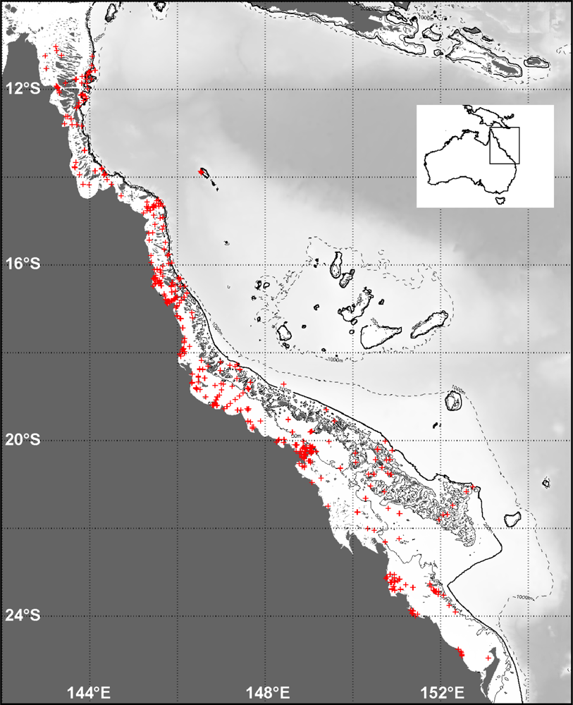
Since sufficient GBR in situ optical data were not readily available for validation purposes, regional measurements of Z_SD collected by the Australian Institute of Marine Science (AIMS) and the Queensland Department of Primary Industries and Fisheries (QDPI) were used to serve as a first order ground-truth for the satellite data products, with over 5,000 records acquired. These data were somewhat biased towards the inshore region (Figure 1), due to the focus of the regional research and monitoring programs, with Z_SD often quite low (<5 m). Such values are not unusual in GBR inshore waters, which experience intermittent high turbidity due to resuspension and flood inputs. Higher Z_SD values were generally found further offshore. The timeframes of the data (1994–1999; 1992–2010) largely pre-dated the MODIS-Aqua satellite data (2002–2010), hence SeaWiFS data (1997–2010) were also used to validate and improve the photic depth product for the GBR ecosystem.

Two operational photic depth algorithms have been implemented into the standard NASA ocean color satellite data processing environment, both of which are available via the SeaWiFS Data Analysis System (SeaDAS; http://oceancolor.gsfc.nasa.gov/seadas): an empirical algorithm based on Case-1 assumptions [21] and a semi-analytical algorithm based on the inherent optical properties (IOPs) of the water column [4]. The IOP approach, where photic depth is described as a function of spectral absorption and backscattering coefficients, was selected for this study as the water-clarity algorithm to determine light penetration depth in eutrophic, Case-2 coastal waters [6]. This algorithm has been tested and validated for oceanic and coastal waters in the Arabian Sea, Monterey Bay, Gulf of Mexico and Yellow Sea [4], but not in the GBR.

In this study, IOPs from the quasi-analytical algorithm (QAA; [2]) were used to determine the depth where 10% of the surface light (PAR) level was still available, Z_10%, which was in turn regionally tuned to Z_SD using “matchups” with in situ Z_SD data. The satellite-to-in situ matchups for the AIMS and QDPI in situ Z_SD dataset were acquired from the NASA Ocean Biology Processing Group (OBPG) [22]. Matchups were generated for both SeaWiFS and MODIS-Aqua. These matchups were generated using the methods and quality assurance procedures described in Bailey and Werdell [23], which included: (1) locating satellite observations made within ± 3-hours of the time of in situ data collection; (2) calculating the filtered median of all unflagged pixels within a 5 × 5 pixel box centered on the in situ target; and (3) excluding any matchups where the coefficient-of-variation of the unflagged satellite pixels exceeded 0.15. To the best of our knowledge, we excluded matchup stations in optically shallow water, where light reflected off of the sea floor contributes to the water-leaving signal observed by the satellite.

A regression of the in situ Z_SD values against the matching satellite estimates of Z_10% was used to adjust the satellite-derived Z_10% to Z_SD. A Type II linear regression (RMA) of log-transformed satellite and in situ data was used to estimate Z_SD for the GBR according to:

$${\text{Z}}_{\text{SD}}=10^\left[\left\{{\text{log}}_{10}\left({\text{Z}}_{10\%}\right)-{\text{a}}_0\right\}/{\text{a}}_1\right]$$

(1)

where a₀ and a₁ are 0.518 and 0.811 for SeaWiFS (N = 235; r² = 0.78; RMSE = 0.148) and 0.529 and 0.816 for MODIS-Aqua (N = 71; r² = 0.83; RMSE = 0.096). This method for regional tuning is ultimately insensitive to our choice of a specific Z_%, as the assignment of percent light level in Lee et al.[4] changes only the absolute magnitude of the depth estimates, not their variability. For example, had we used Z_37% in Equation (1), a₀ and a₁ would be different than reported above, but their derived Z_SD would not. Finally, this GBR-validated Z_SD algorithm was implemented into the SeaDAS environment and applied to the full regional time series of MODIS-Aqua data (2002–2012). Daily, monthly and decadal means and anomalies were generated at 1-km² resolution and analyses undertaken. For the purpose of this study, the analyses focused on the central to southern GBR (S-GBR, 18°S–24°S).

To represent the temporal evolution of water clarity on the S-GBR over the last decade (July 2002 to June 2012), latitude-time Hovmöller diagrams were generated for both the S-GBR continental shelf and inshore lagoon regions. Bathymetry masks were created to limit the spatial domains to 0–200 m and 0–35 m for the shelf and inshore regions, respectively, excluding topographic reef features. Monthly mean Z_SD values were averaged along each ∼0.01° line of latitude (1-km resolution) for each of the selected masked areas. Pixels coinciding with missing values (<3%) and over topographic reef features were ignored in the computation.

To characterize the variability of the satellite-derived Z_SD on the S-GBR, an Empirical Orthogonal Function (EOF) Analysis was performed on the ten-year monthly Z_SD dataset. An EOF Analysis is a statistical technique used to decompose the spatial and temporal variability of time series datasets into a few independent dominant modes, each representing a certain percentage of the total variance of the dataset. In this study, we employed the singular value decomposition (SVD) method [24] to calculate the spatial eigenfunctions and temporal eigenvectors. The former describes the spatial pattern associated with the mode, while the latter provides the corresponding temporal variation, which can be interpreted in relation to physical processes. The EOF assumes that there is no gap in the data time series. Hence, prior to doing the analysis, missing data over small gaps (<3% in total) were filled for each monthly dataset, using a kernel interpolation [25]. The bathymetry mask was used to limit the spatial domain to the shelf area (0–200 m). The long-term (10 years) temporal mean was removed from the time series at each pixel location prior to analysis to reduce the dominant seasonal signal [24].

3. Results and Discussion

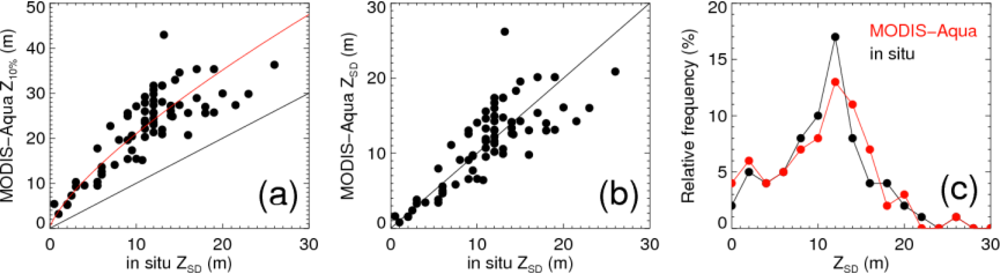
The results of the satellite-to-in situ “matchups” for the AIMS/QDPI Z_SD dataset were far better than expected, given that there had been no regional refinement of the IOP photic depth algorithm. The results showed primarily a simple bias offset between the in situ and satellite retrievals, with similar slopes and intercepts for SeaWiFS and MODIS-Aqua (Equation (1)). Using a linear regression of log-transformed data to generate the GBR-validated Z_SD algorithm eliminated negative values returned for Z_SD when the regression was applied in normal space. Figure 2 shows the MODIS-Aqua GBR satellite-to-in situ matchups tuned using log-transformed data in the regression.

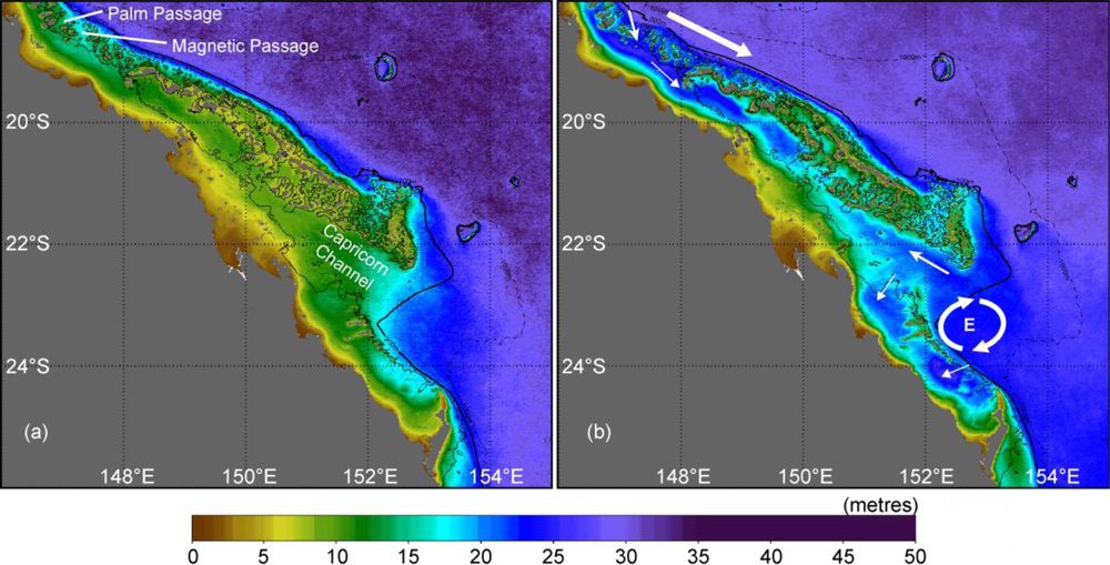
The GBR-validated Z_SD time series of monthly and decadal means generated from MODIS-Aqua data showed considerable seasonality in water clarity, with distinct patterns of spatial distribution. On the GBR shelf, inshore waters were generally more turbid than further offshore, with waters most turbid during March and most transparent during September (Figure 3). This distinct seasonal variation is due to variability in the ocean-atmosphere dynamics, with more turbid waters in the austral summer (Figure 3(a)), the “wet season” on the GBR, when the prevailing north-westerlies and the Coriolis effect result in primarily offshore surface flow of sediment-laden waters from river discharge and increased vertical mixing. During austral winter, or the “dry season” on the GBR, the prevailing southeasterly trade winds dominate, limiting cross-shelf surface flow. Furthermore, seasonal strengthening of the southward-flowing EAC in early spring (September–October), when the opposing trade winds begin to subside [26–28], results in strong intrusions of clear, oligotrophic EAC waters through the Palm and Magnetic Passages in the central GBR [29], with southward flow along the mid-shelf channel (Figure 3(b)). At the southern end of the GBR, the Capricorn Eddy forms most strongly during spring when the EAC strengthens, with resultant intrusions of clear EAC waters into the Capricorn and Curtis Channels [15], further enhancing separation of the inner and outer shelf regions (Figure 3(b)).

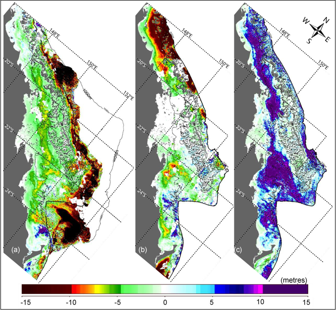
The Z_SD anomalies clearly showed areas and times where water clarity was anomalously poor, following periods of increased cyclonic or storm activity. For example, intense positive anomalies followed excessive storm activity in March 2009, with the cross-shelf extent and turbid water track of Tropical Cyclone (TC) Hamish, a powerful category 5 storm, clearly visible along the continental shelf edge of the S-GBR, even extending offshore as far as the 1,000 m isobath (Figure 4(a)). Similarly, the newly implemented GBR Z_SD product allowed near-realtime tracking of the intrusion of anomalous conditions following TC Yasi (category 5) that impacted the central GBR in February 2011 (Figure 4(b)). In contrast, the strongest negative anomalies occurred in September 2008 (Figure 4(c)), when intrusions of clear oceanic waters appeared particularly intense, both into the central GBR channel and from the south, into the Capricorn and Curtis Channels.

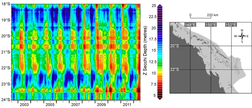
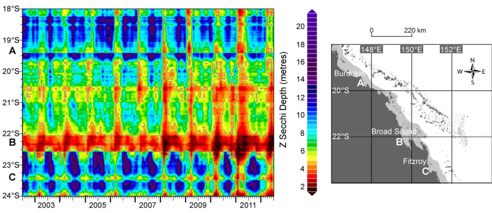
The Hovmöller diagrams illustrate the variation of water clarity on the S-GBR in space (latitude) and time (July 2002 to June 2012), both across the entire continental shelf (Figure 5) and along the inshore region (Figure 6). A distinct seasonal signal is apparent on the S-GBR shelf (Figure 5), with water generally more turbid in late summer (February to April) and clearest in late winter/early spring (August to October). Spatially, mean water clarity across the shelf is higher in latitudinal bands coincident with intrusions of oceanic waters in the central (between 18.25°S and 19.25°S) and southern GBR (between 22.25°S and 23.25°S). However, most notable is the decline in water clarity in recent years, with a significant decrease in mean shelf Z_SD of 2.00 m (from 13.9 m to 11.9 m) over the last decade, after removal of the seasonal signal (F = 10.58; p < 0.0015; n = 120). A progressive increase in space-time for which the average cross-shelf Z_SD values remained below the critical water quality level for the GBR of <10 m Z_SD[8] is also apparent. Poor water clarity was especially pronounced in April to May 2012 (Figure 5), when mean cross-shelf Z_SD values of <8 m were experienced in the S-GBR, declining at locations to as low as 6 m in May, likely due to strong vertical mixing and intrusions onto the shelf of anomalously turbid waters following sustained, strong winds in the greater study region (Australian Bureau of Meteorology, http://www.bom.gov.au/).

On the inner shelf (0–35 m), a distinct seasonal signal is also apparent (Figure 6), along with the turbid water signatures of the seasonal riverine inputs from the Burdekin (∼19.4°S) and Fitzroy Rivers (∼23.5°S), the two largest rivers in Queensland, which had above-median flows for the Burdekin from 2007–2012 and above-median flows for the Fitzroy in 2008 and 2010–2012, respectively. Also clearly visible is Broad Sound (∼22.1°S–22.4°S), an embayment where high tidal energy causes strong vertical mixing of the shallow waters, leading to low water clarity all-year-round. The decline in water clarity in recent years is even more pronounced in this inshore area where a significant decrease in mean inner shelf Z_SD of 2.1 m (from 8.3 m to 6.2 m) occurred over the last decade, after removal of the seasonal signal (F = 10.58; p < 0.0015; n = 120). From summer 2007/08 onwards, the areas and time periods markedly increased where Z_SD values remained below 5 m (Figure 6), which is half of the Z_SD trigger level for GBR waters [8,12]. These negative trends in water clarity coincided with the five years during which the GBR experienced strong La Niña conditions in 2007/08, 2008/09, 2010/11 and 2011/12 (Australian Bureau of Meteorology). In northeastern Australia, La Niña events are typically associated with an earlier onset of and a more vigorous summer monsoon, characterized by enhanced tropical cyclone activity and wetter summers [30–33]. The associated increased river discharge and vertical mixing is likely to be the main reason for the measured decrease in water clarity, especially of the shallow inner shelf waters.

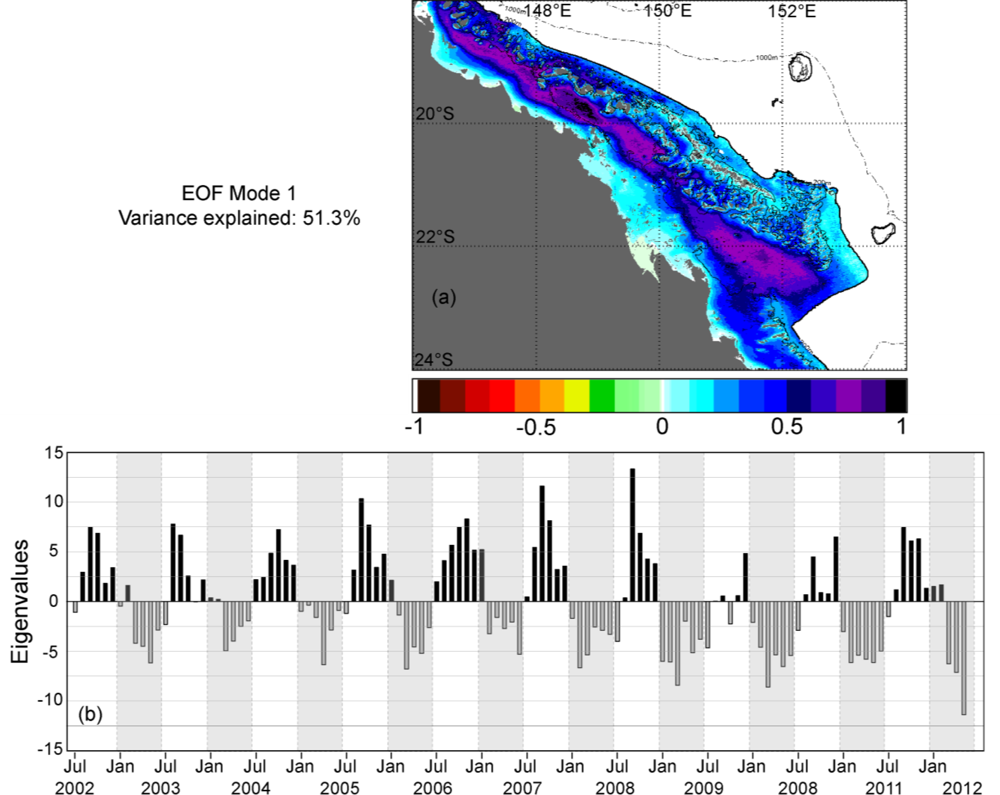
The EOF Analysis decomposed the spatial and temporal variability of the Z_SD time series on the S-GBR shelf over the last decade into a few independent dominant modes, each representing a certain percentage of the total variance of the dataset. Only the first two dominant modes are presented here, explaining 51.3% and 10.7% of the total variance, respectively. Mode 1 (Figure 7), which accounts for over half of the total variance of the dataset, indicates a strong seasonal signal in photic depth variability on the S-GBR, with considerable interannual variation. The spatial pattern (Figure 7(a), normalized from −1.0 to +1.0) shows a consistent phase (positive in Figure 7(a)) across the entire shelf, with the most positive values (purple) in the mid-shelf region. The temporal eigenvectors for Mode 1 (Figure 7(b)) provide the temporal variation associated with the spatial pattern (Figure 7(a)) over the 10-year period. More positive eigenvalues indicate months when the shelf waters were clearer, whereas more negative eigenvalues represent months when water clarity was poorer. The greatest variance explained by Mode 1 occurred at locations where values are most positive in the spatial map (Figure 7(a)), with the clearest waters here during months when the eigenvalues (Figure 7(b)) were most positive, or conversely, the most turbid waters here during months when the eigenvalues were most negative. A pronounced pattern is apparent in the temporal variation, with more turbid waters in the first half of the year, generally from March to May, and clearer waters in the latter half, generally in September and October. Interannual variation is apparent across the time series with a change to reduced water clarity in more recent years.

However, most notable in Figure 7 is that the greatest variation in water clarity occurred along the mid-shelf, not in the inshore region directly exposed to seasonal river outflow, inferring a strong influence of oceanic intrusions during certain months. The combined spatial and temporal patterns show the clearest waters intruding through the Palm and Magnetic Passages and along the mid-shelf channel, and similarly, in the Capricorn Channel in the south. Furthermore, water clarity is generally greatest during early spring (Figure 7(b)), when the EAC strengthens and the southeast trade winds relax. This springtime acceleration of the EAC is known to lead to intrusions in the central GBR [27,29] and further to the south, the Capricorn Eddy forms most strongly and regularly in spring, with associated intrusions up the Capricorn Channel [15,28]. These intrusions onto the mid-shelf would somewhat separate the water bodies of the inner-shelf from the outer shelf waters. During the early months of the year, when the GBR is under the influence of the summer monsoon and associated increased river outflows, northwesterly winds dominate, enhancing cross-shelf flow of more sediment-laden waters. The influence of the strong La Niña conditions experienced over the recent five years is apparent in the interannual variation (Figure 7(b)), where enhanced tropical cyclone activity, wetter summers, stronger northwesterlies and increased vertical mixing have impacted the entire shelf waters for many consecutive months. The dominance of Mode 1 (51.3%) further reinforces the strong influence of the varying physical dynamics on the spatio-temporal patterns of water clarity on the S-GBR.

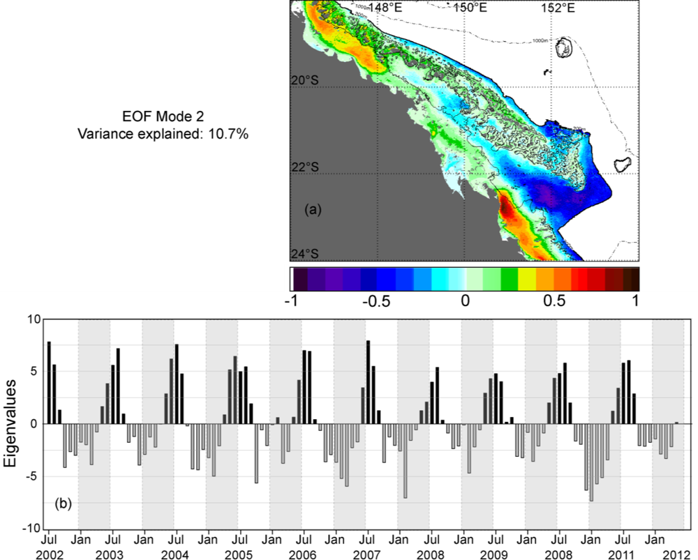
Mode 2 of the EOF Analysis (Figure 8) explains 10.7% of the total variance of Z_SD on the S-GBR shelf over the last decade. The spatial pattern (Figure 8(a), normalized from −1.0 to +1.0) shows generally positive values inshore and along the outer reefs, contrasting with negative values along the shelf edge, the mid-shelf and in the south. The associated temporal eigenvectors for Mode 2 (Figure 8(b)) show generally positive eigenvalues in autumn and winter, the “dry season” on the GBR, with negative eigenvalues in spring and summer during the “wet season”. Hence, during spring/summer for example, the negative eigenvalues combined with positive loadings in the spatial map show areas of poor water clarity and, where combined with negative spatial loadings, show areas of increased water clarity during those same months.

In the central GBR, the greatest variance appeared on the mid-shelf, primarily due to increased vertical mixing and intrusions onto the shelf of more turbid waters during summer, such as occurred when TC Yasi approached the central GBR in January 2011, as opposed to clearer waters in this area during winter. However, the greatest variance explained by Mode 2 occurred in the south, largely representing the offshore and spatial extent of river outflow. Here, the opposing positive/negative values in the spatial map show that the most turbid waters coincided with a strong EAC in summer when clear oceanic waters flowed along the shelf-edge, skirted the Swains reefs in the south and intruded up the Capricorn Channel, containing any large river outflow inshore. This is especially notable in the long wet summer of 2010/11, when southeast Queensland experienced extreme flooding. The 2010–2011 wet season was characterized by extreme events in the GBR region, driven by a very strong La Niña, with the intense and prolonged rainfall resulting in the Fitzroy River having its largest flow in the instrumental record (approximately 38 million ML) [34]. However, of interest is that while the variance explained by Mode 2 appears related to storms and cyclonic events in summer, and consequent increased river discharge, variability in water clarity in the S-GBR was generally not most pronounced directly inshore where Z_SD remained persistently low.

4. Concluding Remarks

The Z_SD product generated from the implementation of the GBR-validated Z_SD algorithm allowed us to produce a long-term time series of water clarity data since 2002. Potential future applications of these data are, e.g., (i) to define baseline ranges of water clarity along and across the GBR to identify and quantify future changes in water clarity as a result of land use practice changes or other environmental changes such as climate change; and (ii) to analyze spatial and temporal patterns of change in reef communities in response to changes in water clarity.