Mapping Vegetation Density in a Heterogeneous River Floodplain Ecosystem Using Pointable CHRIS/PROBA Data


1
Image Processing Laboratory, Department of Earth Physics and Thermodynamics, University of Valencia, P.O. Box 22085, E-46071 Paterna (Valencia), Spain
2
Laboratory for Geo-Information and Remote Sensing, Wageningen University and Research Centre, Droevendaalsesteeg 3, 6708 PB Wageningen, The Netherlands
*
Author to whom correspondence should be addressed.
Remote Sens. 2012, 4(9), 2866-2889; https://doi.org/10.3390/rs4092866
Submission received: 1 August 2012
/
Revised: 14 September 2012
/
Accepted: 17 September 2012
/
Published: 24 September 2012
Abstract
:River floodplains in the Netherlands serve as water storage areas, while they also have the function of nature rehabilitation areas. Floodplain vegetation is therefore subject to natural processes of vegetation succession. At the same time, vegetation encroachment obstructs the water flow into the floodplains and increases the flood risk for the hinterland. Spaceborne pointable imaging spectroscopy has the potential to quantify vegetation density on the basis of leaf area index (LAI) from a desired view zenith angle. In this respect, hyperspectral pointable CHRIS data were linked to the ray tracing canopy reflectance model FLIGHT to retrieve vegetation density estimates over a heterogeneous river floodplain. FLIGHT enables simulating top-of-canopy reflectance of vegetated surfaces either in turbid (e.g., grasslands) or in 3D (e.g., forests) mode. By inverting FLIGHT against CHRIS data, LAI was computed for three main classified vegetation types, ‘herbaceous’, ‘shrubs’ and ‘forest’, and for the CHRIS view zenith angles in nadir, backward (−36°) and forward (+36°) scatter direction. The −36° direction showed most LAI variability within the vegetation types and was best validated, closely followed by the nadir direction. The +36° direction led to poorest LAI retrievals. The class-based inversion process has been implemented into a GUI toolbox which would enable the river manager to generate LAI maps in a semiautomatic way.
1. Introduction
Climate change is expected to have a large impact on water resources and flooding risks of the main rivers in the Netherlands [1]. General circulation models applied on the Rhine river basin predict higher winter discharge and peak flows as a result of increased winter precipitation and earlier snow-melt in the Alps [2,3]. During the 20th century, measures for improvement of river navigation, as well as agricultural development have caused the Rhine to lose its natural meanders while significant parts of the floodplain have been affected by urban development [4,5]. As a result, the capability of the river system to accommodate peak flows has been reduced which leads to increased flooding risks for the floodplains and its hinterland [6].
During the last decades, the water discharge capacity of the river system in the Netherlands has been increased by lowering and widening of the floodplains, removal of hydraulic obstacles in the floodplains and by excavation of secondary channels [7,8]. Concomitantly, these newly developed river floodplains also serve as nature restoration areas, where succession of vegetation leads to highly valued ecosystems [9]. However, floodplain vegetation causes resistance to the water flow within the river floodplains [10]. Because of the complex structure of floodplain vegetation and the accumulation of material caused by sedimentation processes, flood flow velocities decrease and the water surface increases during flooding events [11]. For assessment of current and future river management scenarios in low land rivers like the Rhine in the Netherlands, information on the spatially complex structure and density of floodplain vegetation is a key issue [12].
To intervene with the spontaneous vegetation succession, the concept of Cyclic Floodplain Rejuvenation (CFR) has been introduced for management of the Rhine river system [13]. CFR implies periodic anthropogenic disturbance of floodplain ecosystems through removal of climax vegetation to create more space for water. To support this approach, regular monitoring of the spatial distribution and structure of floodplain vegetation is required for estimating the flow resistance within the floodplain. Flow resistance indicates to what extent the water flow is obstructed and is directly related to vegetation height and density, rigidity of the stems and the presence of leaves [14–18]. For the rivers Rhine and Meuse in the Netherlands, ecotope maps are used for determining flow resistance values of the vegetation, resulting in one roughness value per ecotope object. Currently, ecotope maps are based on digital false colour aerial photographs and ancillary in situ data on flood duration, management, water depth and morphodynamics [19]. However these techniques are time-consuming and no information on spatial variability of vegetation density within the ecotopes is provided.
Alternatively, satellite based Earth observation (EO) can play a major role by providing a quantifiable, spatially-explicit and replicable technique for monitoring and assessing the magnitude of floodplain vegetation density [20,21]. With optical EO data, vegetation properties can be characterised into a few essential structural variables that quantify vegetation density such as leaf area index (LAI), defined as the total of one-sided area of leaves per area (m2/m2) [22]. Particularly in fully vegetated floodplains LAI can be considered as the main parameter that quantifies vegetation density. Consequently, LAI has been proposed to be implemented in flow resistance calculation schemes [18]. The latter author linked LAI with cross-sectional flow velocity, flow depth and plant height to calculate the friction factor for flow inside leafy and woody vegetation on floodplains and wetlands. Implementing spatially-explicit LAI estimates in flow resistance calculation schemes may therefore bypass the need for many elaborative field measurements [20,21].
The retrieval of LAI from EO data is often based on empirical relationships between spectral vegetation indices and ground-based measurements (e.g., [23–25]). These relationships work well under particular viewing and illumination geometry and for specific vegetation phenology, but they tend to produce inaccurate results when applied over a broad range of land cover types and optical and geometric conditions encountered in satellite images [26]. Canopy reflectance is the result of several intricately coupled physical processes and it is therefore difficult to estimate the influence of a single parameter from experimental data (e.g., [27]). Contrary to empirical approaches, radiative transfer (RT) models take the physical features of a plant canopy into account and are therefore more realistic in describing the interaction of solar radiation with vegetation components. A canopy RT model describes the transfer and interactions of solar radiation inside such a canopy and thus provides an explicit link between the structural characteristics of vegetation scattering elements and the canopy reflectance [28]. In these RT models the spectral signal is a function of canopy geometry, defined by canopy structural variables such as LAI, leaf angle distribution and fractional vegetation cover, optical leaf and soil properties, illumination and viewing geometry. LAI is a key variable in describing the density of the scattering elements. In turn, these biophysical variables can be extracted from RT models through model inversion (e.g., [29]).
Apart from the expected enhancement of the physical RT modelling approach for retrieval accuracy, additional gains are to be expected with the use of pointable sensors. Various studies demonstrated that canopy reflectance measurements acquired under different observation angles can yield unique information pertaining to vegetation structure [30–39]. The presence of shadows in the canopy forms an important argument for exploring pointable data because the shadowing effect in vegetated surfaces will result in enhanced reflectance in the backscatter direction and reduced reflectance in the forward scatter direction of the principal plane [40]. Therefore, the combined use of RT methods with pointable imaging spectroscopy data may lead to a more robust approach to map the complex floodplain vegetation structure and density from space.
The ESA’s Compact High Resolution Imaging Spectrometer (CHRIS) on board the Project for On Board Autonomy (PROBA) satellite is a pointable, imaging spectroscopy sensor that was designed as a technology demonstrator [34]. CHRIS is capable of measuring reflected radiation over the visible and near-infrared (NIR) spectra from 406 to 1,035 nm from five different viewing angles (nadir, ±36°, ±55°) by pointing five times to the same target during a single overpass. It can operate in different modes, balancing the number of spectral bands, site of the covered area and spatial resolution because of on-board memory storage reasons. However, being a technology demonstrator, CHRIS does not acquire data on a routine basis but images can be acquired on request. The spacecraft is essentially designed for scientific applications, amongst others for developing new vegetation monitoring strategies. For instance, several studies demonstrated that angular CHRIS data in combination with a RT modelling approach hold promises to monitor LAI over agricultural fields [26,41,42]. Nonetheless, research on quantifying LAI over heterogeneous floodplain ecosystems, taking into account different vegetation types such as species-rich grasslands grading towards shrub and tree encroachments, have rarely garnered attention in the scientific literature.
In this study we aim at characterizing the density variable LAI of a spatially and spectrally complex river floodplain ecosystem using angular CHRIS data. The objective is threefold: (i) to develop a RT model inversion methodology for physically-based mapping of LAI of several vegetation types in a river floodplain ecosystem using pointable CHRIS data (Mode 3: 18 bands with 17 m of spatial resolution); (ii) to explore the added value of the use of the different viewing angles (nadir, ±36°) in the applied methodology; and (iii) to assess the opportunities to apply the methodology developed for a local floodplain to a complete river section at the regional scale.
2. Materials and Methods
2.1. Study Site
The study site is the floodplain Millingerwaard (51°84′N, 5°99′E) along the river Waal, which is the main branch of the river Rhine in the Netherlands (Figure 1). Millingerwaard (700 ha) is one of the main floodplains of the nature reserve Gelderse Poort, with a total surface area of 6700 hectare. Within the Netherlands, the Gelderse Poort serves as important riparian corridor within the Natura 2000 network of the European Union. Before 1990, Millingerwaard was used as an agricultural area with intensively managed grassland and arable crops (e.g., maize). Starting from 1990, agricultural management was gradually reduced and a nature rehabilitation plan was started. By digging out clay deposits from the topsoil, the old patterns of side streams, natural levees and isles were reconstructed in the landscape. Floodplain vegetation was going through natural succession and a regime of grazing by cattle and horses in low densities was introduced. Current vegetation of the Millingerwaard floodplain consists of mixed patches and ecotones, i.e., transitions between communities with a dominance of grass, herbaceous vegetation, dwarf and tall shrubs, and a large softwood forest [43]. Softwood forest in Millingerwaard is dominated by willow trees (Salix fragilis and Salix alba). The forest canopy has an open structure with dense undergrowth (Urtica dioica (stinging nettle), Arctium lappa (greater burdock), Galium aparine (cleavers)) and open water bodies due to the low elevation and high ground water levels. The non-forest vegetation is characterized by a heterogeneous patchy structure of different vegetation succession stages. Dominant species are Urtica dioica, Calamagrostis epigejos (wood small-reed), and Rubus caesius (dewberries). Finally, a limited number of parcels is still in agricultural use. Vegetation types present in Millingerwaard are representative for the vegetation succession stages of the other floodplains within the Gelderse Poort nature reserve. At this moment, the surface area of agricultural land in the complete Gelderse Poort is relatively high compared to that of the Millingerwaard, however, this will change over the coming decade as agricultural management will be changed to a nature management regime.
2.2. CHRIS Data
During the same PROBA overpass five pointable CHRIS images over the Millingerwaard and a large part of the Gelderse Poort (Figure 1) were quasi-simultaneously acquired on 6 September 2005 in Mode 3 under cloud-free conditions around solar noon. Mode 3 is appropriate for vegetation structure mapping as it is characterized by both a high spatial (∼17 m) and high spectral resolution with 18 bands measuring in the visible and NIR wavelengths from 400 to 1,050 nm, thereby covering a region of 13 by 13 km (full swath) [34] (Table 1). CHRIS images were acquired at nadir, ±36°, ±55° nominal viewing zenith angles (VZA) and are named as such hereafter. The actual position of the sensor during the satellite overpass is shown in the polar plot of Figure 2. Negative viewing angles represent measurements in the backscatter direction, where most sunlit canopy is viewed by the sensor; positive viewing angles represent measurements in the forward scatter direction, where most shadowing effects are present. The solar zenith angle during acquisition was 46°. For the purpose of this research, the images of VZA nadir and ±36° were used, because the ±55° images faced a reduction in the common area viewed by the sensor due to a misregistration in the pointing to the target.
Automatic image registration of the CHRIS nadir and ±36° images was performed according to the method of [44] to reference the three separate images to each other. Geometric correction of these three images was carried out with use of 34 ground control points (GCP’s) which were collected from a high spatial resolution (0.5 m) aerial photograph from early spring 2006. Because the CHRIS images were already referenced to each other, the GCP’s were taken from the nadir image only and also applied to the ±36° images. A 2nd order polynomial model with nearest neighbourhood resampling technique was used for geometric correction of the three images which resulted in a control point error of 0.31 pixels. Atmospheric correction of the images was performed according to the method described by [45] using the CHRIS-Box software developed as a plug-in for the BEAM toolbox (Brockmann Consult, http://www.brockmann-consult.de/beam).
2.3. Land Cover Classification of CHRIS nadir Image
Prior to LAI retrieval in canopies comprised of a heterogeneous mix of vegetation types, these vegetation types need to be identified so that the RT model can be parameterized accordingly. By using information from the three observation angles, a map was created that included eight major land cover classes (Table 2). The vegetated classes consisted of ‘bare soil and pioneer communities’, ‘grasses and herbaceous vegetation’, ‘higher herbaceous vegetation’, ‘shrubs’, and ‘forest’. These classes are in accordance to the class definitions used by [11] that serve as a minimum set to estimate flow resistance for river management purposes. The class ‘forest’ represents the areas that consist of pixels with tree cover. The classes ‘water’, ‘build up area’, and ‘arable land’ were added to be able to classify the whole CHRIS image. A summary of all classes and their main characteristics is listed in Table 2, the undertaken steps are shortly explained below.
Maximum likelihood (ML) classification was performed on the CHRIS nadir image to classify the identified land cover classes within the boundaries of Millingerwaard (Figure 1). First, a training data set was defined on which the classification was based. Regions of interest (ROIs) were selected as training data for each land cover class. Field knowledge and aerial photographs of early spring 2006 were used as reference for selecting ROIs. The ROIs consisted of a combination of 10 polygons for each class which were selected with a minimum number of more than 51 pixels. The selection of ROIs was evaluated by computing ROI separability based on the transformed divergence and Jeffries-Matusita Distance of the whole visible and NIR (VNIR) spectrum from the CHRIS nadir image. The separability values showed that the pair of ‘higher herbaceous vegetation’ and ‘grasses and low herbaceous vegetation’ had highly comparable spectral characteristics.
The aerial photographs of 2006 were used as basis for selection of data-points to validate the classification result of the major land cover classes. A set of twenty random sample points was selected per class resulting in the selection of 160 points in total. The distance between two points was set to a minimum of 100 m to prevent choosing points located too close to each other. Finally, classification accuracies and the kappa statistic were calculated for the classified land cover map.
2.4. FLIGHT Model Inversion to Derive LAI
Among RT models, FLIGHT (Forest LIGHT interaction model) is a three dimensional (3D) ray tracing model based on Monte Carlo simulations of photon transport. FLIGHT simulates photon trajectories, starting from a solar source, through successive interactions with the vegetation, to a predetermined sensor viewing angle [46]. The model incorporates the probability of free path, absorption and scattering of photons and accounts for shadowing effect, crown overlapping and multiple scattering between crowns. Within the crown, photons are scattered based on probability density functions. The individual photons are followed until they are either absorbed or exited by the canopy. The model outcome is scene top-of-canopy bi-directional reflectance (BRF) values, the result of a unique stand configuration, solar illumination direction, surface reflection direction and spectral wavelength (λ). FLIGHT can be operated either in 1D or 3D mode. In 1D mode, the vegetation canopy is modelled as turbid medium, which can be seen as a layer that contains a mix of different canopy elements which represent the vegetation density characteristics. Vegetation density of a scene is exclusively controlled by LAI. In 3D mode, the vegetation canopy is modelled as a 3D representation of tree crowns, which are idealized by volumetric primitives of defined shapes with associated shadowing effects. Vegetation density within the volumetric primitives is controlled by LAI and the density of the primitives within a scene is controlled by fractional vegetation cover. This 1D/3D flexibility enables to employ a better representation of patchy landscapes, i.e., homogeneous areas can be simulated in 1D mode while heterogeneous areas (e.g., ‘forest’) can be simulated in 3D mode. In turn, inversion of the model against measured reflectance data allows retrievals of LAI at the sensor sub-pixel scale.
The vegetation classes used in the classification were simplified to form a base map for the class-based model inversion. From the five vegetation classes ‘bare soil and pioneer vegetation’; ‘grasses and low herbaceous vegetation’; ‘higher herbaceous vegetation’; ‘shrubs’; and ‘forest’, the vegetation class ‘bare soil and pioneer vegetation’ was omitted from further analysis because this class does not have a complex structure (i.e., characterized by sparsely distributed, low-growing grassland species) thus the influence on the flow resistance in case of a flooding can be neglected. The two classes ‘grasses and low herbaceous vegetation’ and ‘higher herbaceous vegetation’ which showed a relatively low separability were aggregated into one class, further referred to ‘herbaceous’ vegetation. This led to three distinct vegetation classes ‘herbaceous’, ‘shrubs’ and ‘forest’, for parameterization of FLIGHT. The ‘herbaceous’ and ‘shrubs’ classes were parameterized in 1D mode because of its continuous horizontal distribution, while ‘forest’ was parameterized in 3D mode. For each vegetation class, model parameters; leaf, woody and background spectra; and LAI variable ranges were defined and fed into FLIGHT (Table 3). Vegetation model parameters were defined based on field measurements and ranges of variables were defined based on findings in literature [47–49]. Leaf reflectance and transmittance spectra were measured with an ASD field spectrometer during a field campaign from 28 July till 2 August in 2004. Also tree geometry indicators were measured and are listed in table 3. We assumed that changes in leaf structure and composition of willow trees (>20 years old), as present in Millingerwaard, are small within a period of one year, and that therefore the field measurements match the reflectance spectra of leaves of willow trees in 2005. Additional reflectance spectra of various bark and background types were collected in April 2009 with an ASD field spectrometer. The spectra were resampled to the band settings of the CHRIS sensor.
Model inversion is required in order to retrieve vegetation characteristics from reflectance data through physically based models. Inversion was accomplished by means of a lookup-table (LUT) approach. The LUT provides a simple way of the inversion of a radiative transfer model and also reduces the computational demand compared to the traditional optimization approach [50]. For each VZA and each vegetation class a LUT containing simulated reflectance data was built by means of combining the canopy variables following the steps as provided in Table 2. Given the LUT input parameters, FLIGHT subsequently computed the BRF for 18 spectral bands corresponding to the band settings of the CHRIS sensor. The inversion itself was done by first calculating the root mean square errors (RMSE) between each measured reflectance spectrum from the CHRIS nadir and ±36° images and all simulated BRF spectra as stored in the LUT. Because multiple variable combinations may lead to the same spectra (the problem of ill-posedness), the solution applied here is the average of variable combinations found within less than 10% of the lowest RMSE value. The 10% threshold agrees with several studies that attempted to optimize inversion (e.g., [51–53]). As such, LAI values were pixelwise retrieved per vegetation class for the nadir and the ±36° VZAs. Additionally, RMSE residuals were provided to obtain information about the performance of the retrievals. The residuals reveal the closeness of actual spectral observations to that of the simulated spectra in the inversion; lower residual means a better match. This enabled to compare differences in retrieval performances between angles.
An essential step in asserting the appropriateness of optical EO measurements to partake in the characterization of vegetation density variables is to seek evidence in the validity of the variables. Validation of LAI measurements were derived from a ground sampling campaign which was carried out in first two weeks of august 2004 and 2005 in the Millingerwaard [54]. The 2004 dataset consisted of 13 sample plots of 20 × 20 m in the forest area, which were selected following a random sampling scheme with a minimum of 20 m distance from each other. Each plot was set up according to the VALERI (Validation of Land European Remote Sensing Instruments) protocol [55] and consisted of 12 measurement points per plot. At each point within the plot one measurement in 180° upward direction and one measurement in 180° downward direction were taken with the hemispherical camera. The hemispherical photographs were processed with use of the neural network based software CAN_EYE to calculate the gap fraction and to derive the clumping factor and true LAI values [56]. The 2005 validation dataset acquired in the last week of June consisted of 16 sample plots of 20 × 20 m with more or less homogeneous vegetation cover in ‘herbaceous’, ‘shrubs’ and ‘forest’ vegetation. The sample plots were also set up according to the VALERI protocol. The effective LAI was estimated with use of hemispherical photography and subsequently corrected into true LAI values with use of the average clumping index per plant-functional type from TRAC (Tracing Radiation and Architecture of Canopies) measurements and woody-to-total area ratio from the hemispherical photographs [57]. Thus in total 29 LAI validation points were collected.
2.5. Applying the Method to the Larger Floodplain Area
The final step comprised applying the methodology to all floodplains within the complete river section of the Gelderse Poort nature reserve (Figure 1). RT models are not limited to site or sensor-specific dependencies but it requires that vegetation optical properties are comparable with the calibration area. The same LUT can then be applied to larger floodplain areas without having to compromise on the retrieval quality. To do so, first a land cover classification was made, based on the same training dataset which was used for the Millingerwaard. FLIGHT model inversion was subsequently applied per vegetation class for the Gelderse Poort to derive LAI values. Because of the class-based inversion approach and the broad range of simulations present in the LUT for each vegetation class, covering a large variety of plausible canopies, no additional adjustments had to be made to apply the same methodology to the larger floodplain area. Finally, in view of applying the class-based model inversion approach to images from any imaging spectrometer, the whole methodology has been implemented into a Matlab-based graphical user interface (GUI) toolbox called ARTMO (Automated Radiative Transfer Models Operator) [58]. Hence, with ARTMO LAI maps can be obtained in a semiautomatic way thereby taking the distinct nature of different land cover classes into account.
3. Results
3.1. Classification
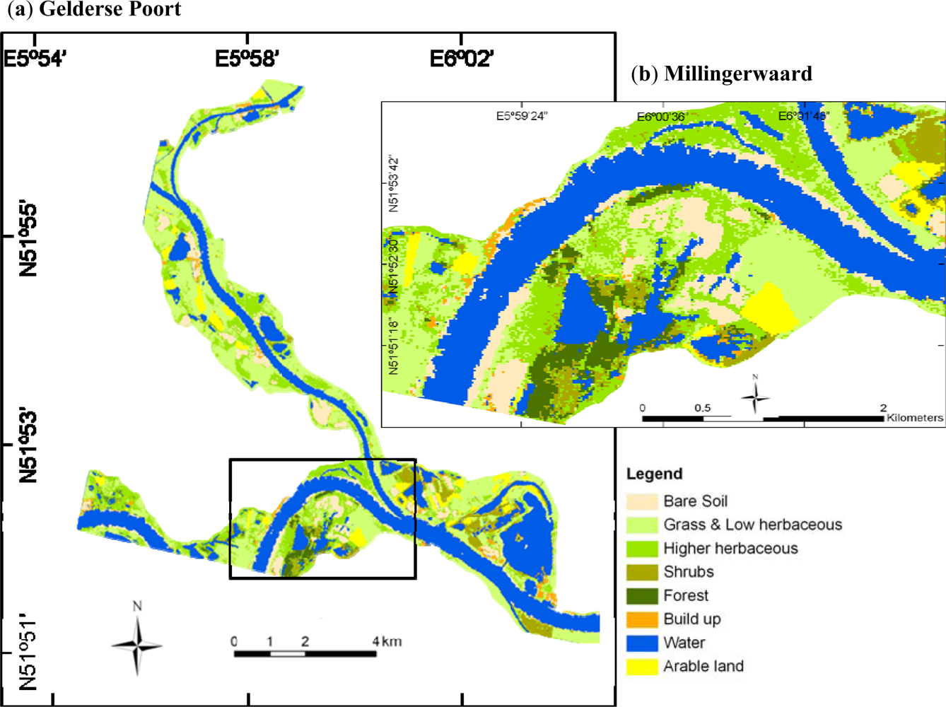
The classified land cover map of the CHRIS nadir image for the Millingerwaard is presented in Figure 3 and has an overall accuracy of 68% and a kappa coefficient of 0.56 (Table 4). Notably, most misclassifications occurred between the ‘grasses and low herbaceous vegetation’ and the ‘higher herbaceous vegetation’, because the spectral characteristics of these classes have similarities and mixing of different vegetation types occurred in the pixels (∼17 m) of the CHRIS image. When merging these two classes, the overall accuracy improved to 73%. The largest part of Millingerwaard was covered by grasses and (low and higher) herbaceous vegetation. Some parts of the river floodplains have recently been excavated and consisted of bare soil. Shrubs and softwood forest surrounded the lakes. Some pieces of land in the eastern part with a rectangular shape and homogeneous land cover represented arable land and agricultural grassland. The remaining part of the area had a heterogeneous land cover with transitions between land cover types on the pixel-level which is characteristic for a natural river floodplain ecosystem.
3.2. Vegetation Class Based Angular LAI Retrievals
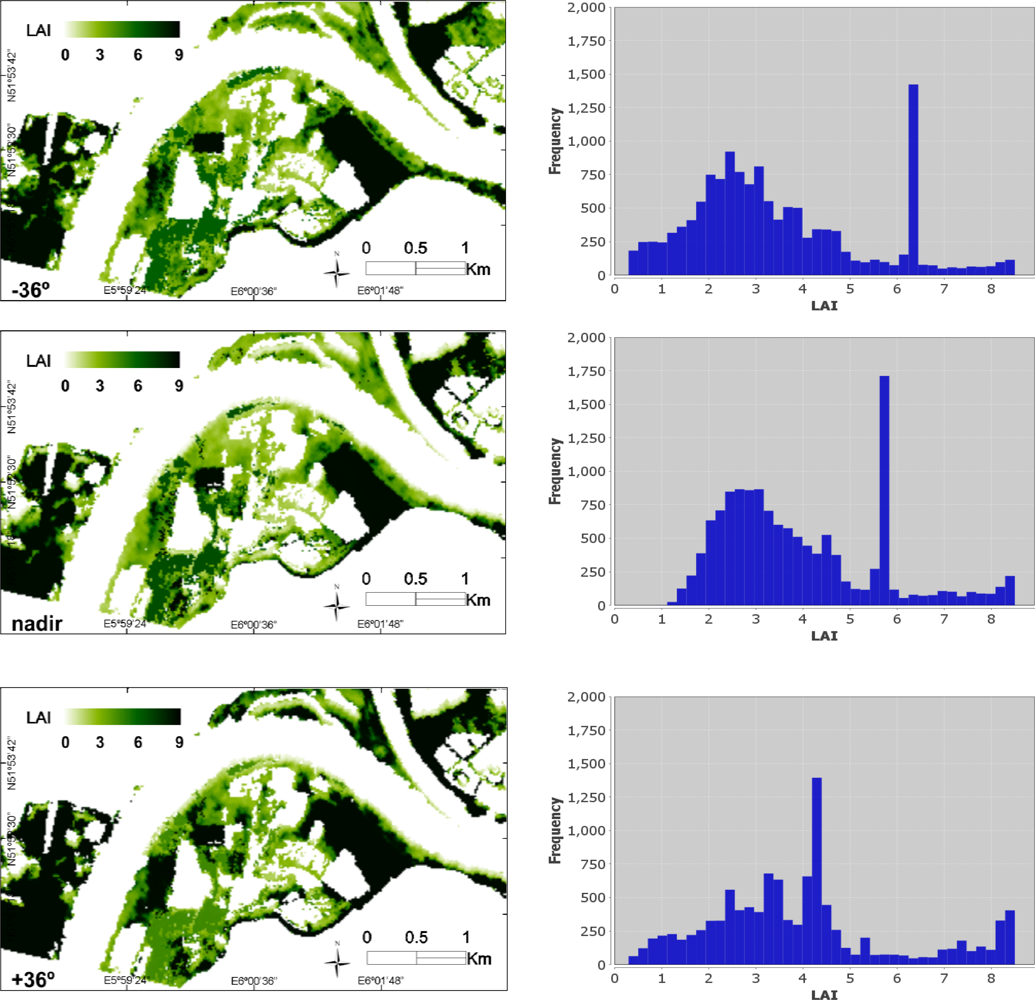
LAI maps were generated through model inversion for the vegetation cover classes of ‘herbaceous’, ‘shrub’ and ‘forest’ vegetation within the Millingerwaard study site and were combined into a single map for each viewing direction (Figure 4 (left)). White parts in the maps represent areas that were not included in one of the three vegetation classes. Large variation in retrieved LAI values could be observed within all the three classes in the river floodplain area, which reinforces the significance of quantifying density at the pixel level. Largest LAI variability was obtained in the −36° VZA, closely followed by the nadir direction, whereas the variation of the inverted values was considerably lower for +36° VZA. Spurious high LAI values between 8 and 9 occurred in several fields and along the dikes. Due to their rectangular shape and homogeneous land cover (Figure 3) it could be deduced that these dense vegetated areas are probably related to intensively managed agricultural fields (mainly maize fields). Similar orders of magnitude were observed along the dike in the south of Millingerwaard, also due to agricultural use. Since the ‘herbaceous’ vegetation class was not parameterized for this vegetation type these agricultural areas are excluded in further analysis. The generated histograms show the LAI distribution of the river floodplain for the three viewing angles (Figure 4 (right)).
From these histograms it can be observed that nadir failed to identify pixels with very low LAI (<1), which are present over the sandy river banks. In case of −36° VZA, LAI values ranged between 0.3 and 6 for the ‘shrubs’ and ‘herbaceous’ areas. Large variations were obtained within the ‘herbaceous’ vegetation class west of the lakes. Peaks in LAI indicated the spatial pattern of shrub encroachment, where the highest values belonged to the fast growing shrub Crataegus monogyna (hawthorn). Also the shrub class around the lakes showed great variation in LAI. This concerned mainly Salix (willow) species which vary in density and height. The ‘forest’ class, which was simulated in 3D, yielded LAI values within a narrow range, between 5 and 7.
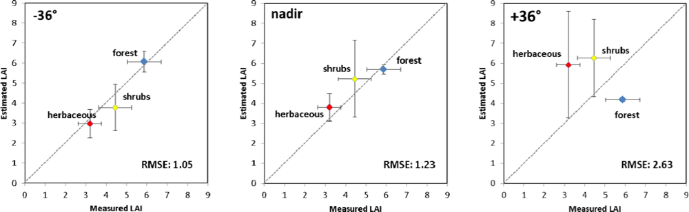
When validating the LAI results, it can be observed from the scatter plots (Figure 5) that the nadir and −36° VZA performed alike, with a somewhat better RMSE accuracy for −36° VZA. The RMSE accuracies were 1.05 for −36° VZA and 1.23 for nadir respectively. Overall, for both viewing angles the retrieved LAI values were overall closely positioned to the 1:1-line. The retrieved LAI values fell within the same range between 2 and 7 as the LAI values obtained with the hemispherical camera (Figure 5). Though, it has to be noted that over the pixels labelled as ‘forest’ hardly variation in LAI was detected. Conversely, the +36° VZA led to considerably poorer accuracies (RMSE: 2.63), suggesting that this viewing angle leads to suboptimal retrievals.
Another way of evaluating the performances of the LAI retrievals is inspecting the RMSE residuals, which were mapped in Figure 6 (left). Although no validation per se, these RMSE maps can give us a better spatial understanding of the success of the inversion process. When comparing the viewing angles it can be noted that nadir and −36° VZAs performed alike, while forward scatter +36° VZA had more difficulty with the inversion. The latter not only led to overall poorer residuals but also delivered considerably more patches with very poor retrievals (dark red spots). This implies that some degree of mismatch between actual spectra and the simulated spectra took place. It suggests that either FLIGHT was not well able to represent the complex shadowing effects in this direction or that a more accurate atmospheric correction regime is needed at this angle. The RMSE maps also suggested that there were no indications that one vegetation class performed worse than the other classes; the image was consistently inverted with some patches (dark red spots) of poorer residuals. These patches typically emerged on landscape edges or on areas with high LAI retrievals. Finally, when looking closer to the residuals at nadir and −36°, despite some patches of poor retrievals, −36° VZA showed slightly better performances throughout the whole image. This can also be observed in the histograms of the residual maps (Figure 6 (right)), where the −36° VZA led to considerably more pixels with very low RMSE values (very left part of histogram).
3.2. LAI Mapping of the Larger Floodplain ‘Gelderse Poort’
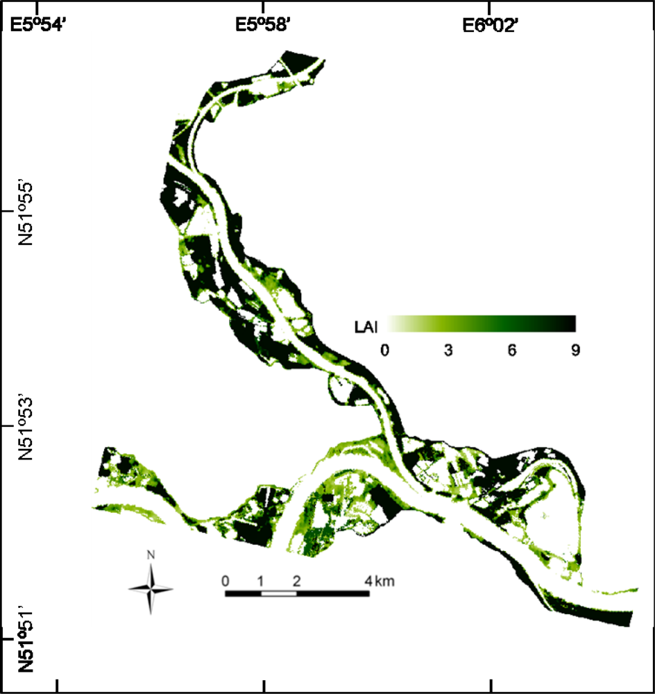
To demonstrate the portability of the class-based model inversion, the complete methodology was applied to the larger floodplain area of the Gelderse Poort nature reserve. This resulted first in a land cover map (Figure 3) and subsequently LAI maps for the three viewing angles for this area. The land cover map reveals that most natural vegetation is present in the southern part of the land cover map. The Millingerwaard floodplain is located here, but the landscape is also characterized by patches of semi-natural grasslands, shrubs, bare soil and lakes and agricultural fields. To the North, the landscape is dominated by agricultural crops and grasslands. These parts have not yet been subject to the natural management regime. The map formed the basis for the class-based LAI retrieval. Figure 7 shows as an example of the LAI map for the −36° VZA, the viewing angle that was best validated and where most variability was perceived. Generated LAI values over the larger floodplain were within the same range as over the Millingerwaard. Large LAI variability can be observed in the more natural areas, especially in the South and South-eastern part of the map, but also in some parts along the river in the centre and North of the map. More northwards, where more agricultural fields were present, areas of high LAI values suggest that these parcels consisted of homogeneous agricultural vegetation cover, such as mature maize fields. Ideally, since these areas probably present a LAI overestimation, these agricultural areas should have been parameterized as an independent LUT class.
4. Discussion
4.1. Vegetation Density Characterization
LAI is one of the main biophysical variables that can be derived from space [22]. At the same time, LAI can be considered as an important proxy of vegetation density, which holds promise for the calculation of flow resistance of river floodplains [18]. Specifically the vegetated areas with high LAI have potential to generate a high accumulation of biomass, and are most critical for the estimation of the hydraulic conductivity of the floodplain. For these areas removal of vegetation under the Cyclic Floodplain Regime could be considered [13]. Moreover, deriving LAI from pointable observations may be beneficial compared to conventional nadir observation because of the ability of controlling the contribution of shadowing effects. For the purpose of quantifying and monitoring LAI over heterogeneous floodplains, we have developed a semiautomatic retrieval strategy on the basis inverting the ray tracing model FLIGHT. The retrieval strategy has been made adjustable to different vegetation classes to account for heterogeneous landscapes and has been implemented into a GUI toolbox called ARTMO [58]. As such, we applied the inversion strategy to nadir and ±36° CHRIS images.
Our results show a prominent spatial and angular variability in LAI values within the studied floodplain across the three pointable CHRIS images (Figure 4). For instance, it appeared that the −36° VZA demonstrated largest variability and best retrieval performances. Particularly subtle LAI variations in case of low LAI were best detected in this viewing configuration (Figure 4 (top)). An explanation for this observation is that the −36° VZA approached the hotspot most closely, which implies the least influence of shadowing effects and therefore a more pronounced first-order scattering, leading to an enhanced richness of subtle variations in reflectance [30,59]. This was particularly notable in the NIR spectral region. Such enhanced subtleties are assumed to be in a way related to an increased sensitivity towards structural variables [60,61], which makes the viewing angle closest to the hotspot of specific interest.
Slightly less accuracy and variability in LAI retrievals was observed in nadir VZA (Figure 4 (middle). The lowest accuracy in LAI retrievals occurred at +36° VZA (Figure 4 (bottom)). In this direction most of the leaf surfaces are shaded, thereby suppressing variations in reflectance and thus sensitivity in assessing foliage density. Similar results but for a coarser resolution of 275 m were obtained with the usage of multi-angular broadband MISR data [62,63]. These studies underlined that the surface anisotropy signatures varied with sun-target-sensor geometry as well as with seasonality due to changes in canopy composition and structure. Other studies [35,64] found increased sensitivities to vegetation structure and reduced understory effects in off-nadir viewing angles when compared to mono-directional nadir data. This evidence of increased sensitivity to vegetation structure supports the observation that the LAI retrievals from −36° VZA led to superior results when compared to the conventional nadir VZA. However, as our results showed that the differences between −36° and nadir direction were rather small, which suggests that in practice nadir observations are still a valid option.
4.2. Combined Classification and Radiative Transfer Modelling Approach
Vegetation classification prior to model inversion proved to be a vital step for proper retrieval of biophysical parameters in heterogeneous or patchy landscapes. Effectively, one of the main drawbacks regarding the usage of RT models is the poor representation of the ensemble of vegetation structural variables and optical properties present in the field (e.g., [65–67]). RT models are typically parameterized for a specific land cover type, e.g., crops, forest, grassland, thereby restricting model inversion to this specific land cover type. However, in patchy or heterogeneous landscapes, such as river floodplains, it cannot be assumed that model parameterization for one vegetation type is valid for the whole landscape. In this respect, the proposed 1D/3D parameterization (along with distinct optical properties) per vegetation class ensures a more accurate representation of the landscape heterogeneity. From the generated LAI maps it can be observed that the three proposed classes of ‘herbaceous’, ‘shrubs’ and ‘forest’ proved to be valid within the floodplain of the Millingerwaard. Though, at the same time the fact that spurious high results appeared over agricultural (maize) areas in the larger region suggests that these areas fell not within the range of simulations that were parameterized according to the ‘herbaceous’ class. For improved LAI retrievals it would therefore be wise to consider these areas as a new class and parameterize the RT model accordingly. In practice this can be easily done in ARTMO.
A difficulty of vegetation class-based inversion is that it relies on a classified map that consists of well-chosen classes and is of sufficient quality. Apart from the enriched information content for retrievals of vegetation density properties, pointable observations can also enhance the classification process itself. However, its potential in the classification process has not been exploited to the fullest yet. In this study, classification was performed on the CHRIS nadir image only. Owing to the advantages of the multi-dimensionality of CHRIS, pointable observations may also be used as input into the classification method. For instance, Duca et al. [68] found that differences in classes were more evident in multi-angular band compositions than in RGB true colour compositions. By using stacked layers of all multi-angular CHRIS observations as classification input instead of relying on solely the nadir image they improved the neural network classification results with 7%. Several other studies demonstrated the strength of multi-angular information in improving land cover classification [30,69,70]. The latter authors improved the classification accuracy with a combination of nadir and off-nadir data, because as such they were better able to catch the canopy characteristics. Given these examples, a next step would be to elaborate on a more standardized protocol using data from pointable imaging spectrometers so that classifications and LAI retrievals can be realized in a more operational way. Besides, a more precise land cover map as base map may also lead to more accurate LAI retrievals. Apart from the here applied Maximum Likelihood classification numerous alternative classifiers exist which may be more successful in heterogeneous areas, such as unsupervised classifiers, support vector machines, fuzzy classifiers, neural networks (see review in [71]). Finally, when moving towards operational use, additional gain in accuracy can be achieved through: (i) synchronizing acquisition of field data with the satellite overpass; (ii) fine-tuning parameterization of vegetation classes for improved class-based model inversion; (iii) analyzing the relevant bands in the classification and inversion to minimize redundancy (e.g., see [72,73]); and (iv) optimizing the inversion strategy through more powerful cost functions and regularization options.
4.3. Towards Spaceborne River Floodplain Monitoring
Overall, this study profited from the availability of pointable hyperspectral CHRIS data and the advantages of the RT approach. With a physical model, the specific background and vegetation spectral characteristics for each vegetation type were taken into account, which makes LAI retrievals more accurate [41]. Because no additional in situ calibration data sets were needed for this RT approach, the class-based model inversion was easily applied to the larger area of the Gelderse Poort, which demonstrated the suitability of this approach to map the floodplains of the whole river catchment.
While CHRIS data were successfully inverted into LAI, it should nonetheless not be forgotten that PROBA is not an operational spacecraft but was designed as a technology demonstrator. In fact PROBA was initially intended as a one year mission [34]. Currently no new multi-angular imaging spectrometer missions are planned to be launched. Conversely, there is a growing trend to design a new generation of spaceborne imaging spectrometers with pointable capabilities. EnMAP is such an example with ±30° off-nadir pointing capabilities that aims to deliver operational data products [74]. In addition, another upcoming spaceborne system, named Vegetation and Environmental New micro Spacecraft (VENμS), also has pointable capabilities within the range of 30° along and across track and will be launched in 2013 [75]. For both of these sensors, vegetation monitoring of both crops and natural vegetation will be an important application domain. Our results support that off-nadir images benefit to the retrieval of LAI and may therefore be of specific interest in view of these upcoming pointable sensors. Further study is required to investigate the viewing angle effect on RT model inversion of vegetation properties, including the consequences for changing temporal resolutions.
Regardless of progress with respect to refined LAI mapping, eventually one comprehensive flow resistance map is demanded by the river manager, which implies the collection of auxiliary information such a vegetation height [18]. Therefore, a next research step would be to explore data assimilation approaches whereby LAI can be combined with other relevant structural variables that can be derived from space. For instance, Straatsma et al. [12] and Forzieri et al. [20] used a fusion of airborne spectral and altimetry data sets to estimate roughness input parameters such as vegetation height and vegetation density, and subsequently used these data as input into a hydrodynamic model to compute flow resistance values of a local river floodplain. It is foreseen that in the forthcoming years it will become possible to upscale these approaches using spaceborne instruments, e.g., in combination with SAR data [21,76,77]. The advantages of relying on spaceborne optical data are ample; it offers a standardized, spatially-explicit and repeatable monitoring scheme that can cover complete river catchments with high spatial detail. Benefitting from the enriched information present in the backscatter direction, it is beyond doubt that operational pointable sensors (e.g., EnMAP, VENμS) will play an important role in vegetation monitoring programmes. Given this all, further research efforts should lie in elaborating on the compatibility of hydrodynamic models with spaceborne-derived input variables.
5. Conclusions
New methods are required to automate and streamline the time-consuming process of flow resistance calculation caused by vegetation in river floodplains. Deriving leaf area index (LAI), a proxy of vegetation density that can be quantified from space, holds promise for that purpose. Pointable imaging spectrometers possess advanced capabilities to derive LAI under a preferred viewing angle. A methodology for mapping LAI has been developed on the basis of inverting the ray tracing model FLIGHT against pointable CHRIS images, thereby taking the plant structural characteristics of different vegetation classes into account. The approach was applied to a heterogeneous river floodplain area that grades from semi-natural grasslands towards shrub and tree encroachments. The CHRIS nadir image was first classified into three distinct vegetation classes (‘herbaceous’, ‘shrubs’, ‘forest’) that formed the basis for class-based model inversion. By configuring FLIGHT per vegetation class, a more accurate representation of the heterogeneous nature of a river floodplain can be achieved, i.e., ‘herbaceous’ and ‘shrubs’ were simulated in 1D mode while ‘forest’ was simulated in 3D mode. LAI values were subsequently pixelwise and class-based derived through model inversion, and this was carried out for each view zenith angle (VZA: nadir, ±36°) separately. LAI retrievals matched best with validation data at −36° backscatter direction (RMSE: 1.05), which is the viewing angle that was positioned near to the solar position, closely followed by nadir VZA (RMSE: 1.23). Most LAI variability was observed in these two viewing angles. This suggests that in the absence of pointable observations nadir-based observations would be perfectly appropriate for vegetation density monitoring applications. The forward scatterer +36° VZA led to considerably poorer retrievals (RMSE: 2.63) and is not recommended to be used for quantifying vegetation density. The herein proposed methodology has been implemented in a software package ARTMO; thereby, LAI maps over larger areas were generated in a semi-automatic way, while at the same time the heterogeneous nature of the landscape and the viewing configurations of the sensor have been properly interpreted. This approach opens floodplain monitoring opportunities in view of upcoming operational sensors with pointing capabilities such as EnMAP and VENμS.
Acknowledgments
J. Verrelst is supported by the FP7-PEOPLE-IEF-2009 grant (Grant Agreement 252237). This work was partially supported by projects AYA2010-21432-C02-01 and CICYT-2010 funded by the Spanish Ministry of Science and Innovation. This research is part of the project Urban Regions in the Delta 636 funded by the Netherlands Organisation for Scientific Research (NWO). J. P. Rivera is acknowledged for technical support. We also appreciate the valuable suggestions of the reviewers.
References
- Straatsma, M.; Schipper, A.; Van der Perk, M.; Van den Brink, C.; Leuven, R.; Middelkoop, H. Impact of value-driven scenarios on the geomorphology and ecology of lower Rhine floodplains under a changing climate. Landscape Urban. Plann 2009, 92, 160–174. [Google Scholar]
- Tol, R.S.J.; Van Der Grijp, N.; Olsthoorn, A.A.; van der Werff, P.E. Adapting to climate: A case study on riverine flood risks in the Netherlands. Risk Anal 2003, 23, 575–583. [Google Scholar]
- Bronstert, A. Floods and climate change: Interactions and impacts. Risk Anal 2003, 23, 545–557. [Google Scholar]
- Pinter, N.; Van der Ploeg, R.R.; Schweigert, P.; Hoefer, G. Flood magnification on the River Rhine. Hydrol. Process 2006, 20, 147–164. [Google Scholar]
- Disse, M.; Engel, H. Flood events in the Rhine basin: Genesis, influences and mitigation. Nat. Hazards 2001, 23, 271–290. [Google Scholar]
- Middelkoop, H.; Daamen, K.; Gellens, D.; Grabs, W.; Kwadijk, J.C.J.; Lang, H.; Parmeti, B.W.A.H.; Schädler, B.; Schulla, J.; Wilke, K. Impact of climate change on hydrological regimes and water resources management in the Rhine basin. Clim. Change 2001, 49, 105–128. [Google Scholar]
- Silva, W.; Klijn, F.; Dijkman, J. Room for the Rhine Branches in The Netherlands; What the Research Has Taught Us; RIZA report 03; RIZA: Arnhem, The Netherlands, 2001. [Google Scholar]
- Van Stokkom, H.T.C.; Smits, A.J.M. Flood Defense in the Netherlands: A New Era, a New Approach. In Flood Defence; Wu, B., Wang, Z., Wang, G., Huang, G.G.H., Fang, H., Huang, J., Eds.; Science Press: New York, NY, USA, 2002; pp. 34–47. [Google Scholar]
- Kooistra, L.; Wamelink, G.W.W.; Schaepman-Strub, G.; Schaepman, M.E.; Dobben, H.F.; van Aduaka, U.; Batelaan, O. Assessing and predicting biodiversity in a floodplain ecosystem: Assimilation of net primary prodution derived from imaging spectrometer data into a dynamic vegetation model. Remote Sens. Environ 2008, 112, 2118–2130. [Google Scholar]
- Baptist, M.J.; Penning, W.E.; Duel, H.; Smits, A.J.M.; Geerling, G.W.; van der Lee, G.E.M.; van Alphen, J.S.L. Assessment of the effects of cyclic floodplain rejuvenation on flood levels and biodiversity along the Rhine river. River Res. Appl 2004, 20, 285–297. [Google Scholar]
- Geerling, G.W.; Kater, E.; Van den Brink, C.; Baptist, M.J.; Ragas, A.M.J.; Smits, A.J.M. Nature rehabilitation by floodplain excavation: The hydraulic effect of 16 years of sedimentation and vegetation succession along the Waal River, NL. Geomorphology 2008, 99, 317–328. [Google Scholar]
- Straatsma, M.W.; Baptist, M.J. Floodplain roughness parameterization using airborne laser scanning and spectral remote sensing. Remote Sens. Environ 2008, 112, 1062–1080. [Google Scholar]
- Duel, H.; Baptist, M.J.; Penning, W.E. Cyclic Floodplain Rejuvenation: A New Strategy Based on Floodplain Measures for Both Flood Risk Management and Enhancement of the Biodiversity of the River Rhine; NCR Publication; NCR: Delft, The Netherlands, 2001; p. 14. [Google Scholar]
- Petryk, S.; Bosmajian, G.B. Analysis of flow through vegetation. J. Hydraul. Div 1975, 101, 871–884. [Google Scholar]
- Thompson, G.T.; Roberson, J.A. A theory of flow resistance for vegetated channels. Trans. ASABE 1976, 19, 288–293. [Google Scholar]
- Pasche, E.; Rouvé, G. Overbank flow with vegetatively roughened flood plains. J. Hydraul. Eng 1985, 111, 1262–1278. [Google Scholar]
- Kouwen, N.; Fathi-Moghadam, M. Friction factors for coniferous trees along rivers. J. Hydraul. Eng 2000, 126, 732–740. [Google Scholar]
- Järvelä, J. Determination of flow resistance caused by nonsubmerged woody vegetation. Int. J. River Basin Man 2004, 2, 61–70. [Google Scholar]
- Van Velzen, E.H.; Jesse, P.; Cornelissen, P.; Coops, H. Stromingsweerstand Vegetatie in Uiterwaarden, Deel 1 Handboek; RIZA Rapport, RIZA: Arnhem, The Netherlands, 2003; p. 28. [Google Scholar]
- Forzieri, G.; Guarnieri, L.; Vivoni, E.R.; Castelli, F.; Preti, F. Spectral-ALS data fusion for different roughness parameterizations of forested floodplains. River Res. Appl 2011, 27, 826–840. [Google Scholar]
- Forzieri, G.; Castelli, F.; Preti, F. Advances in remote sensing of hydraulic roughness. Int. J. Remote Sens 2012, 33, 630–654. [Google Scholar]
- Jonckheere, I.; Fleck, S.; Nackaerts, K.; Muysa, B.; Coppin, P.; Weiss, M.; Baret, F. Review of methods for in situ leaf area index determination Part I. Theories, sensors and hemispherical photography. Agric. For. Meteorol 2004, 121, 19–35. [Google Scholar]
- Baret, F.; Guyot, G. Potentials and limits of vegetation indices for LAI and APAR assessment. Remote Sens. Environ 1991, 35, 161–173. [Google Scholar]
- Broge, N.H.; Leblanc, E. Comparing prediction power and stability of broadband and hyperspectral vegetation indices for estimation of green leaf area index and canopy chlorophyll density. Remote Sens. Environ 2001, 76, 156–172. [Google Scholar]
- Im, J.; Jensen, J. R.; Jensen, R. J.; Gladden, J.; Waugh, J.; Serrato, M. Vegetation cover analysis of hazardous waste sites in utah and arizona using hyperspectral remote sensing. Remote Sens 2012, 4, 327–353. [Google Scholar]
- Verrelst, J.; Schaepman, M.E.; Koetz, B.; Kneubühler, M. Angular sensitivity analysis of vegetation indices derived from CHRIS/PROBA data. Remote Sens. Environ 2008, 112, 2341–2353. [Google Scholar]
- Verrelst, J.; Schaepman, M.; Malenovsky, Z.; Clevers, J. Effects of woody elements on forest canopy chlorophyll content retrieval. Remote Sens. Environ 2010, 114, 647–656. [Google Scholar]
- Ross, J. The Radiation Regime and Architecture of Plant Stands; Dr W. Junk Publishers: The Hague, The Netherlands, 1981. [Google Scholar]
- Kempeneers, P.; Zarco-Tejada, P.J.; North, P.R.J.; de Backer, S.; Delalieux, S.; Sepulcre-Canto, G.; Morales, F.; van Aardt, J.A.N.; Sagardoy, R.; Coppin, P.; Scheunders, P. Model inversion for chlorophyll estimation in open canopies from hyperspectral imagery. Int. J. Remote Sens 2008, 29, 5093–5111. [Google Scholar]
- Sandmeier, S.; Deering, D.W. Structure analysis and classification of boreal forests using airborne hyperspectral BRDF data from ASAS. Remote Sens. Environ 1999, 69, 281–295. [Google Scholar]
- Diner, D.J.; Asner, G.P.; Davies, R.; Knyazikhin, Y.; Muller, J.-P.; Nolin, A.W.; Pinty, B.; Schaaf, C.B.; Stroeve, J. New directions in earth observing: Scientific applications of multiangle remote sensing. Bull. Amer. Meteor. Soc 1999, 80, 2209–2228. [Google Scholar]
- Chen, J.M.; Liu, J.; Leblanc, S.G.; Lacaze, R.; Roujean, J.-L. Multi-angular optical remote sensing for assessing vegetation structure and carbon absorption. Remote Sens. Environ 2003, 84, 516–525. [Google Scholar]
- Diner, D.J.; Braswell, B.H.; Davies, R.; Gobron, N.; Hu, J.; Jin, Y.; Kahn, R.A.; Knyazikhin, Y.; Loeb, N.; Muller, J-P.; Nolin, A.W.; Pinty, B.; Schaaf, C.B.; Seiz, G.; Strove, J. The value of multiangle measurements for retrieving structurally and radiatively consistent properties of clouds, aerosols, and surfaces. Remote Sens. Environ 2005, 97, 495–518. [Google Scholar]
- Barnsley, M.J.; Settle, J.J.; Cutter, M.A.; Lobb, D.R.; Teston, F. The PROBA/CHRIS mission: A low-cost smallsat for hyperspectral multiangle observations of the earth surface and atmosphere. IEEE Trans. Geosci. Remote Sens 2004, 42, 1512–1520. [Google Scholar]
- Heiskanen, J. Tree cover and height estimation in the Fennoscandian tundra–taiga transition zone using multiangular MISR data. Remote Sens. Environ 2006, 103, 97–114. [Google Scholar]
- Pocewicz, A.; Vierling, L.A.; Lentile, L.B.; Smith, R. View angle effects on relationships between MISR vegetation indices and leaf area index in a recently burned ponderosa pine forest. Remote Sens. Environ 2007, 107, 322–333. [Google Scholar]
- Chopping, M.; Moisen, G.G.; Su, L.; Laliberte, A.; Rango, A.; Martonchik, J.V.; Peters, D.P.C. Large area mapping of southwestern forest crown cover, canopy height, and biomass using the NASA Multiangle Imaging Spectro-Radiometer. Remote Sens. Environ 2008, 112, 2051–2063. [Google Scholar]
- Verrelst, J.; Schaepman, M.E.; Clevers, J.G.P.W. Spectrodirectional Minnaert-k retrieval using CHRIS-PROBA data. Can. J. Remote Sens. 2010, 36, 631–644. [Google Scholar]
- Verrelst, J.; Clevers, J.G.P.W.; Schaepman, M.E. Merging the Minnaert-k parameter with spectral unmixing to map forest heterogeneity with CHRIS/PROBA data. IEEE Trans. Geosci. Remote Sens 2010, 48, 4014–4022. [Google Scholar]
- Sandmeier, S.; Müller, C.; Hosgood, B.; Andreoli, G. Physical mechanisms in hyperspectral BRDF data of grass and watercress. Remote Sens. Environ 1998, 66, 222–233. [Google Scholar]
- Dorigo, W.; Richter, R.; Baret, F.; Bamler, R.; Wagner, W. Enhanced automated canopy characterization from hyperspectral data by a novel two step radiative transfer model inversion approach. Remote Sens 2009, 1, 1139–1170. [Google Scholar]
- Migdall, S.; Bach, H.; Bobert, J.; Wehrhan, M. Inversion of a canopy reflectance model using hyperspectral imagery for monitoring wheat growth and estimating yield. Precis. Agr 2009, 10, 508–524. [Google Scholar]
- Verrelst, J.; Geerling, G.W.; Sykora, K.V.; Clevers, J.G.P.W. Mapping of aggregated floodplain plant communities using image fusion of CASI and LiDAR data. Int. J. Appl. Earth Obs. Geoinf 2009, 11, 83–94. [Google Scholar]
- Ma, J.; Chan, J.C.-W.; Canters, F. Fully automatic subpixel image registration of multiangle CHRIS/PROBA Data. IEEE Trans. Geosci. Remote Sens 2010, 48, 2829–2839. [Google Scholar]
- Guanter, L.; Alonso, L.; Moreno, J. A method for the surface reflectance retrieval from PROBA/CHRIS data over land: Application to ESA SPARC campaigns. IEEE Trans. Geosci. Remote Sens 2005, 43, 2908–2917. [Google Scholar]
- North, P.R.J. Three-dimensional Forest light interaction model using a Monte Carlo method. IEEE Trans. Geosci. Remote Sens 1996, 34, 946–956. [Google Scholar]
- Broadbent, E.N.; Zarin, D.J.; Asner, G.P.; Peña-Claros, M.; Cooper, A.; Littell, R. Recovery of forest structure and spectral properties after selective logging in lowland Bolivia. Ecol. Appl 2006, 16, 1148–1163. [Google Scholar]
- Gensuo, J.J.; Burke, I.C.; Goetz, A.F.H.; Kaufmann, M.R.; Kindel, B.C. Assessing spatial patterns of forest fuel using AVIRIS data. Remote Sens. Environ 2006, 102, 318–327. [Google Scholar]
- Guerschman, J.P.; Hill, M.J.; Renzullo, L.J.; Barrett, D.J.; Marks, A.S.; Botha, E.J. Estimating fractional cover of photosynthetic vegetation, non-photosynthetic vegetation and bare soil in the Australian tropical savanna region upscaling the EO-1 Hyperion and MODIS sensors. Remote Sens. Environ 2009, 113, 928–945. [Google Scholar]
- Kimes, D.S.; Knyazikhin, Y.; Privette, J.L.; Abuelgasim, A.A.; Gao, F. Inversion methods for physically-based models. Remote Sens. Rev 2000, 18, 381–439. [Google Scholar]
- Combal, B.; Baret, F.; Weiss, M. Improving canopy variables estimation from remote sensing data by exploiting ancillary information. Case study on sugar beet canopies. Agronomie 2002, 22, 205–215. [Google Scholar]
- Richter, K.; Atzberger, C.; Vuolo, F.; Weihs, P.; D’Urso, G. Experimental assessment of the Sentinel-2 band setting for RTM-based LAI retrieval of sugar beet and maize. Can. J. Remote Sens 2009, 35, 230–247. [Google Scholar]
- Vohland, M.; Mader, S.; Dorigo, W. Applying different inversion techniques to retrieve stand variables of summer barley with PROSPECT + SAIL. Int. J. Appl. Earth Obs. Geoinf 2010, 12, 71–80. [Google Scholar]
- Schaepman, M.E.; Wamelink, G.W.W.; Dobben, H.F.; van Gloor, M.; Schaepman-Strub, G.; Kooistra, L.; Clevers, J.G.P.W.; Schmidt, A.M.; Berendse, F. River floodplain vegetation scenario development using imaging spectroscopy derived products as input variables in a dynamic vegetation model. Photogramm. Eng. Remote Sensing 2007, 73, 1179–1188. [Google Scholar]
- Justice, C.; Belward, A.; Morisette, J.; Lewis, P.; Privette, J.; Baret, F. Developments in the ‘validation’ of satellite sensor products for the study of the land surface. Int. J. Remote Sens 2000, 21, 3383–3390. [Google Scholar]
- Mengesha, T.; Schaepman, M.E.; De Bruin, S.; Zurita-Milla, R.; Kooistra, L. Ground Validation of Biophysical Products Using Imaging Spectroscopy in Softwood Forests. Proceedings of the VALERI Workshop, Avignon, France, 10 March 2005. [CD-ROM]..
- Clevers, J.G.P.W.; Kooistra, L. AHS2005: The 2005 Airborne Imaging Spectroscopy Campaign in the Millingerwaard, the Netherlands; CGI Report 2008-001; Centre for Geo-Information, Wageningen University: Wageningen, The Netherlands, 2008. [Google Scholar]
- Verrelst, J.; Rivera, J.P.; Alonso, L.; Moreno, J. ARTMO: An Automated Radiative Transfer Models Operator Toolbox for Automated Retrieval of Biophysical Parameters through Model Inversion. Proceedings of 7th EARSeL Workshop on Imaging Spectrometry, Edinburgh, UK, 11–13 April 2011.
- Dorigo, W.A. Improving the robustness of cotton status characterisation by radiative transfer model inversion of multi-angular CHRIS/PROBA data. IEEE J. Sel. Top. Appl. Earth Obs. Remote Sens 2012, 5, 18–29. [Google Scholar]
- Weiss, M.; Baret, F.; Myneni, R.B.; Pragnère, A.; Knyazikhin, Y. Investigation of a model inversion technique to estimate canopy biophysical variables from spectral and directional reflectance data. Agronomie 2000, 20, 3–22. [Google Scholar]
- Simic, A.; Chen, J.M. Refining a hyperspectral and multiangle measurement concept for vegetation structure assessment. Can. J. Remote Sens 2008, 34, 174–191. [Google Scholar]
- Liesenberg, V.; Galvão, L.S.; Ponzoni, F.J. Variations in reflectance with seasonality and viewing geometry: Implications for classification of Brazilian savanna physiognomies with MISR/Terra data. Remote Sens. Environ 2007, 107, 276–286. [Google Scholar]
- Xavier, A.S.; Galvão, L.S. View angle effects on the discrimination of selected Amazonian land cover types from a principal-component analysis of MISR spectra. Int. J. Remote Sens 2005, 26, 3797–3811. [Google Scholar]
- Rautiainen, M.; Lang, M.; Mõttus, M.; Kuusk, A.; Nilson, T.; Kuusk, J.; Lükk, T. Multi-angular reflectance properties of a hemiboreal forest: An analysis using CHRIS PROBA data. Remote Sens. Environ 2008, 112, 2627–2642. [Google Scholar]
- Gond, V.; De Pury, D.G.G.; Veroustraete, F.; Ceulemans, R. Seasonal variations in leaf area index, leaf chlorophyll, and water content; Scaling-up to estimate fAPAR and carbon balance in a multilayer, multispecies temperate forest. Tree Phys 1999, 19, 673–679. [Google Scholar]
- Soudani, K.; François, C.; le Maire, G.; Le Dantec, V.; Dufrêne, E. Comparative analysis of IKONOS, SPOT, and ETM+ data for leaf area index estimation in temperate coniferous and deciduous forest stands. Remote Sens. Environ 2006, 102, 161–175. [Google Scholar] [Green Version]
- Zhang, Q.; Xiao, X.; Braswell, B.; Linder, E.; Baret, F.; Moore, B., III. Estimating light absorption by chlorophyll, leaf and canopy in a deciduous broadleaf forest using MODIS data and a radiative transfer model. Remote Sens. Environ 2005, 99, 357–371. [Google Scholar]
- Duca, R.; Del Frate, F. Hyperspectral and multiangle CHRIS-PROBA images for the generation of land cover maps. IEEE Trans. Geosci. Remote Sens 2008, 46, 2857–2866. [Google Scholar]
- Braswell, B.H.; Hagena, S.C.; Frolkinga, S.E.; Salas, W.A. A multivariable approach for mapping sub-pixel land cover distributions using MISR and MODIS: Application in the Brazilian Amazon region. Remote Sens. Environ 2003, 87, 243–265. [Google Scholar]
- Galvão, L.S.; Ponzoni, F.J.; Liesenberg, V.; Dos Santos, J.R. Possibilities of discriminating tropical secondary succession in Amazônia using hyperspectral and multiangular CHRIS/PROBA data. Int. J. Appl. Earth Obs. Geoinf 2009, 11, 8–14. [Google Scholar]
- Lu, D.; Weng, Q. A survey of image classification methods and techniques for improving classification performance. Int. J. Remote Sens 2007, 28, 823–870. [Google Scholar]
- Thenkabail, P.S.; Lyon, G.J.; Huete, A. Advances in Hyperspectral Remote Sensing of Vegetation and Agricultural Croplands. In Hyperspectral Remote Sensing of Vegetation; Thenkabail, P.S., Lyon, G.J., Huete, A., Eds.; CRC Press: Boca Raton, FL, USA, 2011. [Google Scholar]
- Huang, J.; Zeng, Y.; Kuusk, A.; Wu, B.; Dong, L.; Mao, K.; Chen, J. Inverting a forest canopy reflectance model to retrieve the overstorey and understorey leaf area index for forest stands. Int. J. Remote Sens 2011, 32, 7591–7611. [Google Scholar]
- Stuffler, T.; Kaufmann, C.; Hofer, S.; Förster, K.P.; Schreier, G.; Mueller, A.; Eckardt, A.; Bach, H.; Penné, B.; Benz, U.; Haydn, R. The EnMAP hyperspectral imager-An advanced optical payload for future applications in Earth observation programmes. Acta Astronaut 2007, 61, 115–120. [Google Scholar]
- Hermann, I.; Pimstein, A.; Karnieli, A.; Cohen, Y.; Alchanatis, V.; Bonfil, D.J. LAI assessment of wheat and potato by VENμS and Sentinel-2 bands. Remote Sens. Environ 2011, 115, 2141–2151. [Google Scholar]
- Peduzzi, A.; Wynne, R.H.; Thomas, V.A.; Nelson, R.F.; Reis, J.J.; Sanford, M. Combined use of airborne lidar and DBInSAR data to estimate LAI in temperate mixed forests. Remote Sens 2012, 4, 1758–1780. [Google Scholar]
- Salvia, M.; Franco, M.; Grings, F.; Perna, P.; Martino, R.; Karszenbaum, H.; Ferrazzoli, P. Estimating flow resistance of wetlands using SAR images and interaction models. Remote Sens 2009, 1, 992–1008. [Google Scholar]
Figure 1.
The study area which is located in the east of the Netherlands, indicated on the CHRIS nadir image in true colour band composition (R: 675.2 nm, G: 551.7 nm, B: 490.5 nm). The red circle represents the river floodplains of Millingerwaard. The black outlined river area overlain on the CHRIS nadir image represents the nature reserve the Gelderse Poort.

Figure 2.
Polar plot showing the actual positions of the five angular CHRIS images during acquisition on 6 September 2005. The solar zenith angle was 46°, the solar azimuth angle 170°.
Figure 2.
Polar plot showing the actual positions of the five angular CHRIS images during acquisition on 6 September 2005. The solar zenith angle was 46°, the solar azimuth angle 170°.

Figure 3.
Maximum likelihood classification result of the CHRIS nadir image of the (a) Gelderse Poort and (b) Millingerwaard (indicated with the black square) into major land cover types.
Figure 3.
Maximum likelihood classification result of the CHRIS nadir image of the (a) Gelderse Poort and (b) Millingerwaard (indicated with the black square) into major land cover types.

Figure 4.
LAI maps (left) and derived histograms for LAI<8.5 (right) of Millingerwaard for the backward scattering direction (−36° VZA) (top), the nadir direction (middle) and the forward scattering direction (+36° VZA) (down), derived with FLIGHT model inversion.
Figure 4.
LAI maps (left) and derived histograms for LAI<8.5 (right) of Millingerwaard for the backward scattering direction (−36° VZA) (top), the nadir direction (middle) and the forward scattering direction (+36° VZA) (down), derived with FLIGHT model inversion.

Figure 5.
Mean validation results and standard deviation of the estimated LAI obtained with FLIGHT model inversion, plotted against the measured LAI values obtained with the hemispherical camera for the backward scattering direction (−36° VZA), the nadir direction and the forward scattering direction (+36° VZA).

Figure 6.
Maps of minimum RMSEs for LAI retrievals (left) and derived histograms for <8.5 (right) of Millingerwaard for the backward scattering direction (−36° VZA) (top), the nadir direction (middle) and the forward scattering direction (+36° VZA) (down), derived with FLIGHT model inversion.
Figure 6.
Maps of minimum RMSEs for LAI retrievals (left) and derived histograms for <8.5 (right) of Millingerwaard for the backward scattering direction (−36° VZA) (top), the nadir direction (middle) and the forward scattering direction (+36° VZA) (down), derived with FLIGHT model inversion.

Figure 7.
LAI map and histogram for the backward scattering direction (−36° VZA), derived with FLIGHT model inversion after applying to the Gelderse Poort area.
Figure 7.
LAI map and histogram for the backward scattering direction (−36° VZA), derived with FLIGHT model inversion after applying to the Gelderse Poort area.


Table 1.
CHRIS specifications for Land Mode 3; general information and centre wavelength (CHRISmid) and full-width-half-maximum (FWHM).
| Sampling | Image Area | View Angles | Spectral Bands | Spectral Range | ||||||||||||||
|---|---|---|---|---|---|---|---|---|---|---|---|---|---|---|---|---|---|---|
| ∼ 17 m @ 556 km altitude | 13 × 13 km (744 × 748 pixels) | 5 nominal angles @ ±55°, ±36°, 0° | 18 bands with 6–33 nm width | 438–1,035 nm | ||||||||||||||
| CHRISmid(nm) | 442 | 490 | 530 | 551 | 570 | 631 | 661 | 672 | 697 | 703 | 709 | 742 | 748 | 781 | 872 | 895 | 905 | 1,019 |
| FWHM (nm) | 9 | 9 | 9 | 10 | 8 | 9 | 11 | 11 | 6 | 6 | 6 | 7 | 7 | 15 | 18 | 10 | 10 | 33 |
| Class Name | Class Characteristics | |
|---|---|---|
| 1 | Bare soil and pioneer vegetation | mainly sand |
| 2 | Grasses and low herbaceous vegetation | vegetation < 1 m |
| 3 | Higher herbaceous vegetation | vegetation between 1 m and 2 m |
| 4 | Shrubs | shrubs and trees < 5 m |
| 5 | Forest | trees > 5 m |
| 6 | Water | water |
| 7 | Build up | streets, houses |
| 8 | Arable land | maize |
Table 3.
FLIGHT model parameters and variables, and input spectra. Fcover: fractional vegetation cover, LAI: leaf area index, PV: photosynthetic vegetation, 1D: 1dimensional, 3D: three dimensional; DBH: diameter breast height. Details about the FLIGHT parameters can be found in [46].
| Class Name | Input Spectra | ||
|---|---|---|---|
| Leaf | Background | Bark | |
| Herbaceous | Calamagrostis epigejos | 0.95*forest background + 0.05*sandy soil | |
| Shrubs | Salix alba | average (water, grass & forest background) | Salix alba |
| Forest | Salix alba | forest background | Salix alba |
| Class Name | Variables | Fixed Parameters | |||
|---|---|---|---|---|---|
| Fcover (%) | LAI (m2/m2) | PV (%) | Scene | Leaf Size (m) | |
| Herbaceous | 20–100; step: 2 | 0.2–10; step: 0.1 until 5; step: 0.5 until 10 | 100 | 1D | 0.027 |
| Shrubs | 20–100; step: 2 | 0.2–10; step: 0.1 until 5; step: 0.5 until 10 | 70 | 1D | 0.02 |
| Forest | 20–100; step: 2 | 0.2–10; step: 0.1 until 5; step: 0.5 until 10 | 70 | 3D | 0.02 |
| Fixed Parameters Tree Geometry (m) | |
|---|---|
| Crown shape | ellipsoid |
| Crown radius | 3 |
| Centre to top distance | 3 |
| Height to first branch: | 1 |
| Min: | |
| Max: | 4 |
| Trunk DBH | 0.4 |
| Ground Truth | Bare soil | Grass & Low Herbaceous | Higher Herbaceous | Shrubs | Forest | Agricultural | Water | Build up |
|---|---|---|---|---|---|---|---|---|
| Bare soil | 11 | 1 | 2 | 3 | ||||
| Grass & low herbaceous | 3 | 19 | 6 | 5 | 1 | 3 | 1 | 1 |
| Higher herbaceous | 1 | 8 | 1 | 1 | ||||
| Shrubs | 2 | 9 | 1 | |||||
| Forest | 2 | 4 | 16 | 1 | 3 | |||
| Agricultural | 1 | 17 | 1 | |||||
| Water | 3 | 1 | 1 | 18 | ||||
| Build up | 2 | 11 |
Share and Cite
MDPI and ACS Style
Verrelst, J.; Romijn, E.; Kooistra, L. Mapping Vegetation Density in a Heterogeneous River Floodplain Ecosystem Using Pointable CHRIS/PROBA Data. Remote Sens. 2012, 4, 2866-2889. https://doi.org/10.3390/rs4092866
AMA Style
Verrelst J, Romijn E, Kooistra L. Mapping Vegetation Density in a Heterogeneous River Floodplain Ecosystem Using Pointable CHRIS/PROBA Data. Remote Sensing. 2012; 4(9):2866-2889. https://doi.org/10.3390/rs4092866
Chicago/Turabian StyleVerrelst, Jochem, Erika Romijn, and Lammert Kooistra. 2012. "Mapping Vegetation Density in a Heterogeneous River Floodplain Ecosystem Using Pointable CHRIS/PROBA Data" Remote Sensing 4, no. 9: 2866-2889. https://doi.org/10.3390/rs4092866