Allometric Scaling and Resource Limitations Model of Tree Heights: Part 2. Site Based Testing of the Model

 ,
, 
Abstract
:
1. Introduction
2. Data
2.1. Field Measurements
2.2. LVIS Data
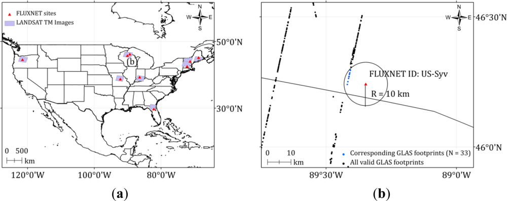
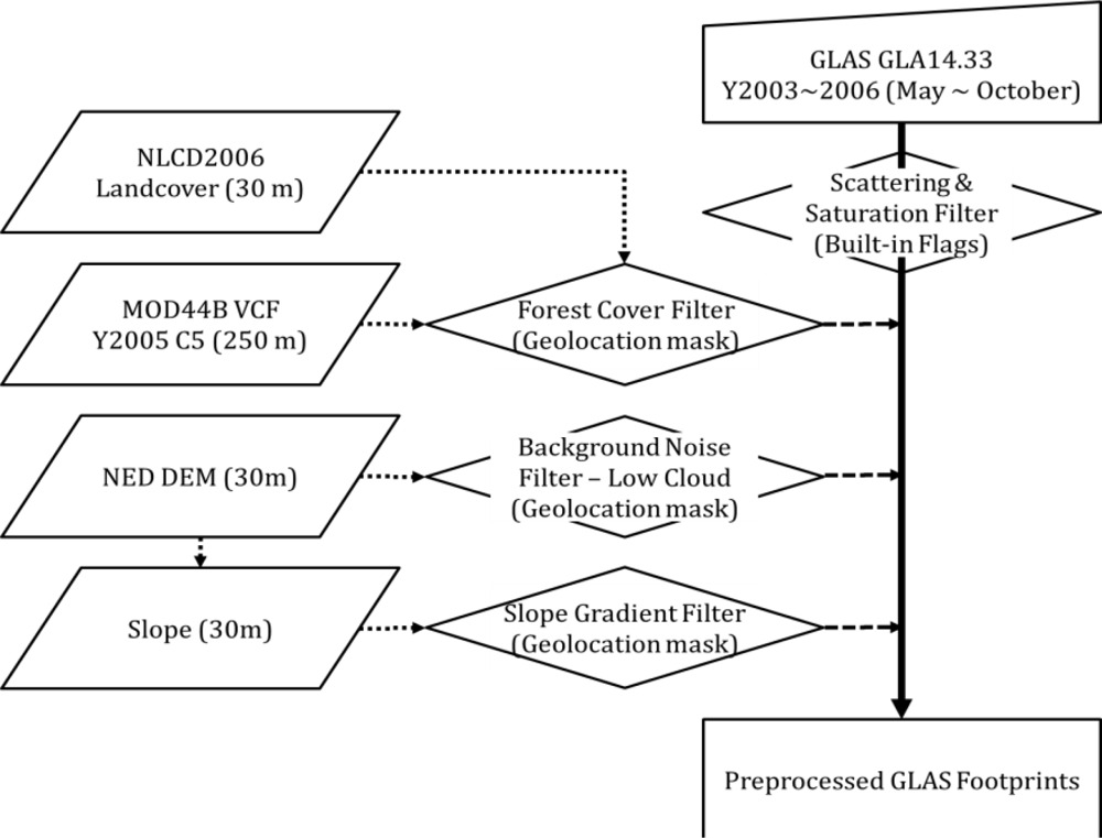
2.3. GLAS Data
2.4. Input Data for the ASRL Model
2.4.1. FLUXNET Data
2.4.2. DAYMET Data
2.4.3. Ancillary Data for the ASRL Model (LAI and DEM)
3. Methods
3.1. GLAS Metric Selection
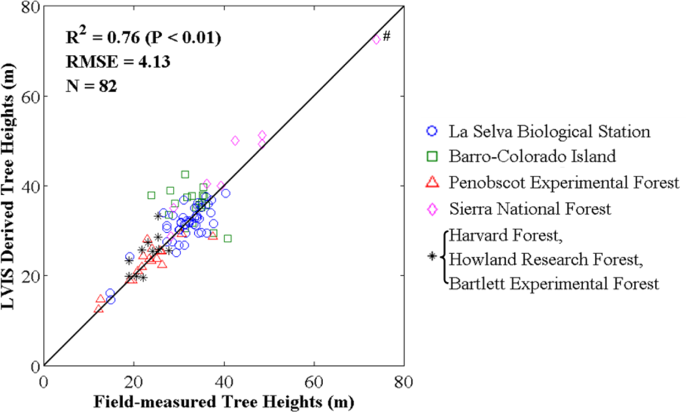
3.1.1. Comparison between Field-Measured and LVIS Tree Heights
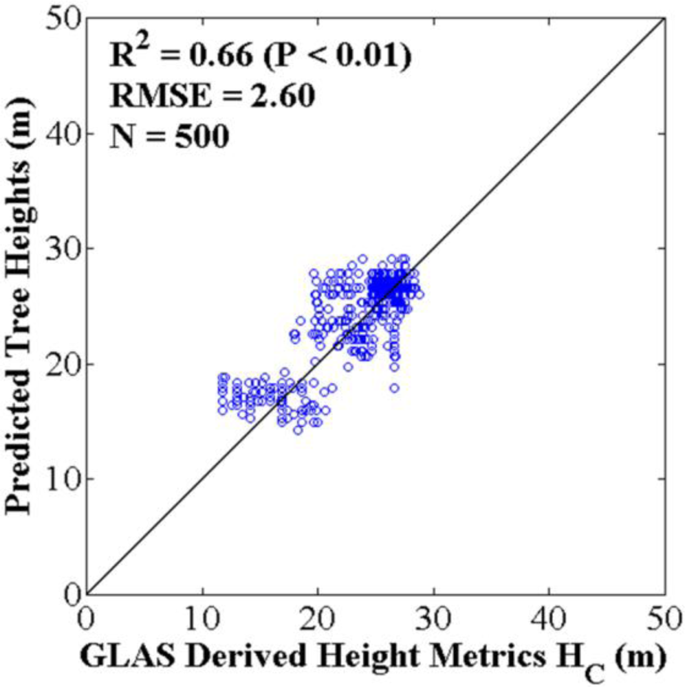
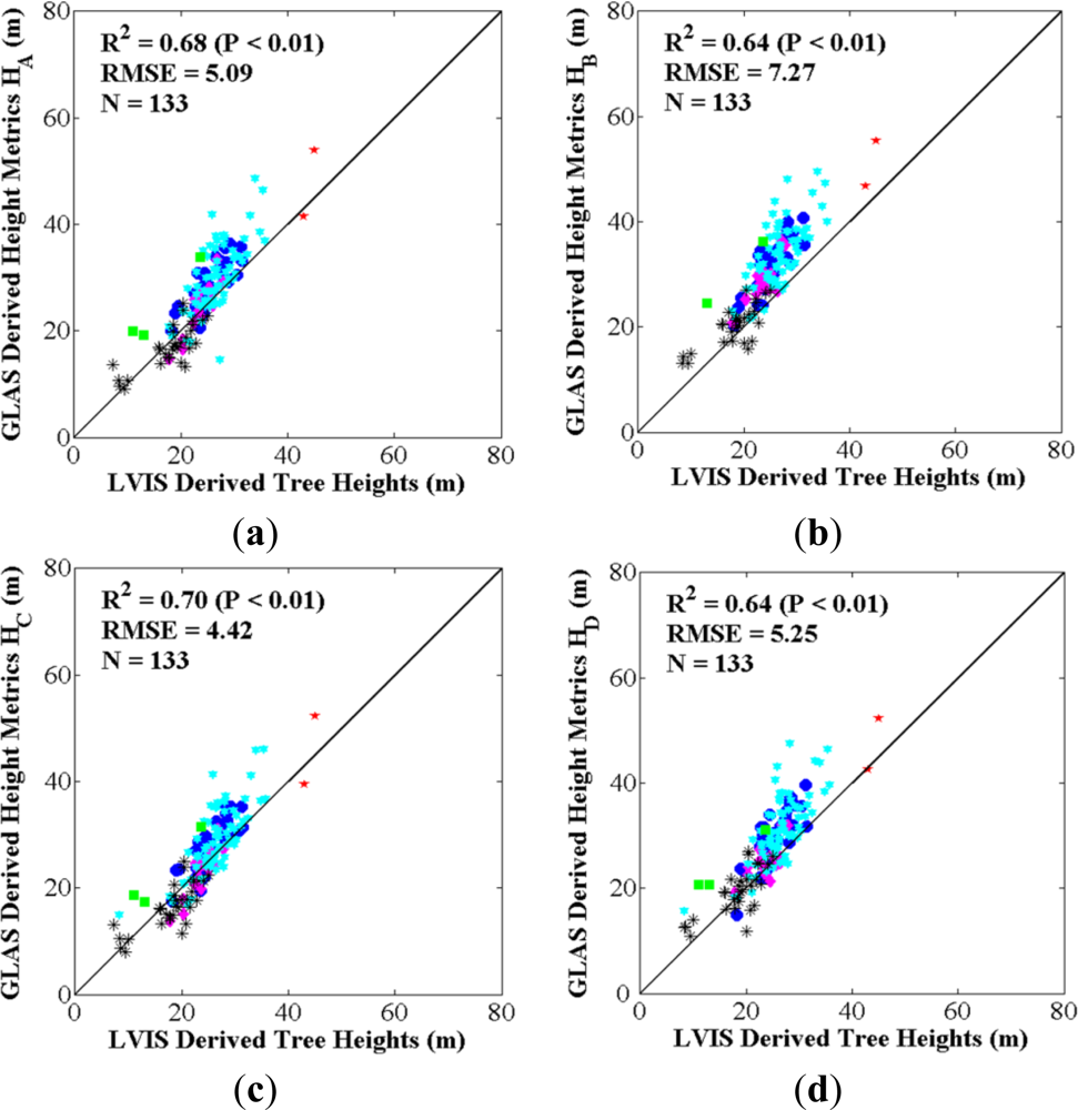
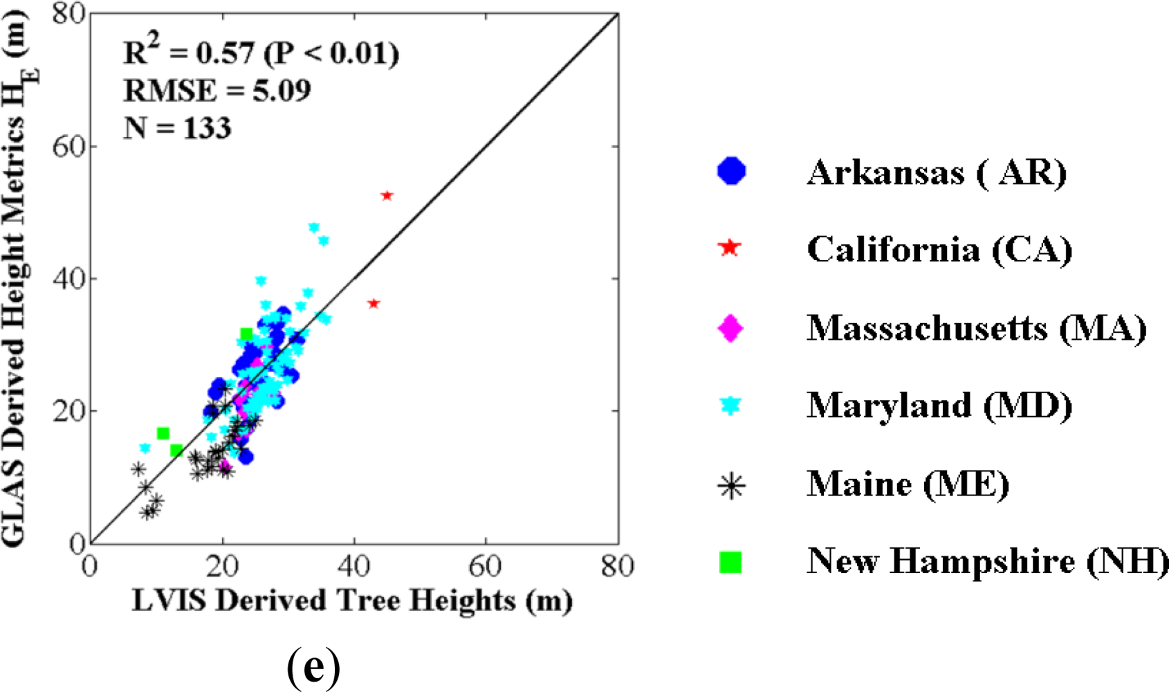
3.1.2. Comparison between LVIS Tree Heights and GLAS Height Metrics
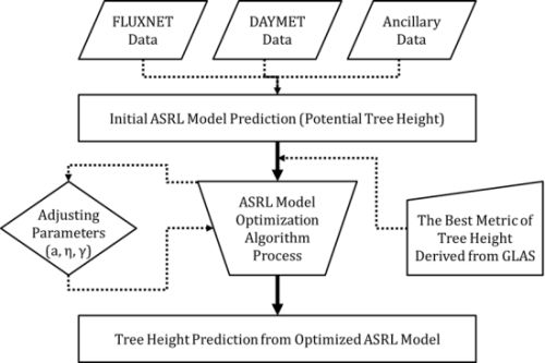
3.2. ASRL Model Optimization
3.2.1. Initial ASRL Model Predictions (Potential Tree Heights)
3.2.2. Optimized ASRL Model Predictions
3.3. Evaluation of the Optimized ASRL Model Predictions
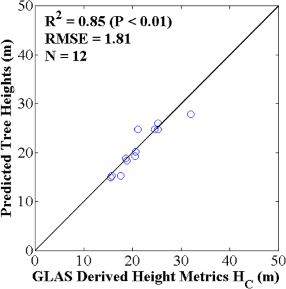
3.3.1. Two-Fold Cross Validation Approach
3.3.2. Bootstrapping Approach
4. Results and Discussion
4.1. Best GLAS Height Metric from Inter-Comparisons with Field-Measured and LVIS Tree Heights
4.2. Optimized ASRL Model Predictions and Evaluations
5. Concluding Remarks
Supplementary Information
remotesensing-05-00202-s001.pdfAcknowledgments
References
- Clark, D.B.; Clark, D.A. Landscape-scale variation in forest structure and biomass in a tropical rain forest. Forest Ecol. Manage 2000, 137, 185–198. [Google Scholar]
- Drake, J.B.; Dubayah, R.O.; Clark, D.B.; Knox, R.G.; Blair, J.B.; Hofton, M.A.; Chazdon, R.L.; Weishampel, J.F.; Prince, S.D. Estimation of tropical forest structural characteristics using large-footprint lidar. Remote Sens. Environ 2002, 79, 305–319. [Google Scholar]
- Muraoka, H.; Koizumi, H. Satellite Ecology (SATECO)-linking ecology, remote sensing and micrometeorology, from plot to regional scale, for the study of ecosystem structure and function. J. Plant Res 2009, 122, 3–20. [Google Scholar]
- Laumonier, Y.; Edin, A.; Kanninen, M.; Munandar, A.W. Landscape-scale variation in the structure and biomass of the hill dipterocarp forest of Sumatra: Implications for carbon stock assessments. Forest Ecol. Manage 2010, 259, 505–513. [Google Scholar]
- Rautiainen, A.; Wernick, I.; Waggoner, P.E.; Ausubel, J.H.; Kauppi, P.E. A National and international analysis of changing forest density. Plos One 2011, 6. [Google Scholar] [CrossRef]
- Gonzalez, P.; Tucker, C.J.; Sy, H. Tree density and species decline in the African Sahel attributable to climate. J. Arid Environ 2012, 78, 55–64. [Google Scholar]
- Liski, J.; Korotkov, A.V.; Prins, C.F.L.; Karjalainen, T.; Victor, D.G.; Kauppi, P.E. Increased carbon sink in temperate and boreal forests. Climatic Change 2003, 61, 89–99. [Google Scholar]
- Kauppi, P.E.; Rautiainen, A.; Korhonen, K.T.; Lehtonen, A.; Liski, J.; Nojd, P.; Tuominen, S.; Haakana, M.; Virtanen, T. Changing stock of biomass carbon in a boreal forest over 93 years. Forest Ecol. Manage 2010, 259, 1239–1244. [Google Scholar]
- Rautiainen, A.; Saikku, L.; Kauppi, P.E. Carbon gains and recovery from degradation of forest biomass in European Union during 1990–2005. Forest Ecol. Manage 2010, 259, 1232–1238. [Google Scholar]
- Pan, Y.D.; Birdsey, R.A.; Fang, J.Y.; Houghton, R.; Kauppi, P.E.; Kurz, W.A.; Phillips, O.L.; Shvidenko, A.; Lewis, S.L.; Canadell, J.G.; et al. A large and persistent carbon sink in the world's forests. Science 2011, 333, 988–993. [Google Scholar]
- Goetz, S.; Dubayah, R. Advances in remote sensing technology and implications for measuring and monitoring forest carbon stocks and change. Carbon Manage 2011, 2, 231–244. [Google Scholar]
- Kauppi, P.E. New, low estimate for carbon stock in global forest vegetation based on inventory data. Silva Fenn 2003, 37, 451–457. [Google Scholar]
- Kauppi, P.E.; Ausubel, J.H.; Fang, J.Y.; Mather, A.S.; Sedjo, R.A.; Waggoner, P.E. Returning forests analyzed with the forest identity. Proc. Natl. Acad. Sci. USA 2006, 103, 17574–17579. [Google Scholar]
- Lefsky, M.A. A global forest canopy height map from the Moderate Resolution Imaging Spectroradiometer and the Geoscience Laser Altimeter System. Geophys. Res. Lett. 2010, 37. [Google Scholar] [CrossRef]
- Simard, M.; Pinto, N.; Fisher, J.B.; Baccini, A. Mapping forest canopy height globally with spaceborne lidar. J. Geophys. Res-Biogeosci. 2011, 116. [Google Scholar] [CrossRef]
- Saatchi, S.S.; Harris, N.L.; Brown, S.; Lefsky, M.; Mitchard, E.T.A.; Salas, W.; Zutta, B.R.; Buermann, W.; Lewis, S.L.; Hagen, S.; et al. Benchmark map of forest carbon stocks in tropical regions across three continents. Proc. Natl. Acad. Sci. USA 2011, 108, 9899–9904. [Google Scholar]
- Kempes, C.P.; West, G.B.; Crowell, K.; Girvan, M. Predicting maximum tree heights and other traits from allometric scaling and resource limitations. Plos One 2011, 6. [Google Scholar] [CrossRef] [Green Version]
- Jung, S.-E.; Kwak, D.-A.; Park, T.; Lee, W.-K.; Yoo, S. Estimating crown variables of individual trees using airborne and terrestrial laser scanners. Remote Sens 2011, 3, 2346–2363. [Google Scholar]
- Straub, C.; Koch, B. Estimating single tree stem volume of Pinus sylvestris using airborne laser scanner and multispectral line scanner data. Remote Sens 2011, 3, 929–944. [Google Scholar]
- Treuhaft, R.N.; Chapman, B.D.; dos Santos, J.R.; Goncalves, F.G.; Dutra, L.V.; Graca, P.M.L.A.; Drake, J.B. Vegetation profiles in tropical forests from multibaseline interferometric synthetic aperture radar, field, and lidar measurements. J. Geophys. Res-Atmos. 2009, 114. [Google Scholar] [CrossRef]
- Treuhaft, R.N.; Goncalves, F.G.; Drake, J.B.; Chapman, B.D.; dos Santos, J.R.; Dutra, L.V.; Graca, P.M.L.A.; Purcell, G.H. Biomass estimation in a tropical wet forest using Fourier transforms of profiles from lidar or interferometric SAR. Geophys. Res. Lett. 2010, 37. [Google Scholar] [CrossRef]
- Baccini, A.; Goetz, S.J.; Walker, W.S.; Laporte, N.T.; Sun, M.; Sulla-Menashe, D.; Hackler, J.; Beck, P.S.A.; Dubayah, R.; Friedl, M.A.; et al. Estimated carbon dioxide emissions from tropical deforestation improved by carbon-density maps. Nature Clim. Change 2012, 2, 182–185. [Google Scholar]
- Zhang, G.; Ganguly, S.; Nemani, R.; White, M.; Milesi, C.; Wang, W.; Saatchi, S.; Yu, Y.; Myneni, R.B. A simple parametric estimation of live forest aboveground biomass in California using satellite derived metrics of canopy height and Leaf Area Index. Geophys. Res. Lett. 2013. under review.. [Google Scholar]
- Lefsky, M.A.; Harding, D.J.; Keller, M.; Cohen, W.B.; Carabajal, C.C.; Espirito-Santo, F.D.; Hunter, M.O.; de Oliveira, R. Estimates of forest canopy height and aboveground biomass using ICESat. Geophys. Res. Lett. 2005, 32. [Google Scholar] [CrossRef]
- Lefsky, M.A.; Keller, M.; Pang, Y.; de Camargo, P.B.; Hunter, M.O. Revised method for forest canopy height estimation from Geoscience Laser Altimeter System waveforms. J. Appl. Remote Sens. 2007, 1. [Google Scholar] [CrossRef]
- Moorcroft, P.R.; Hurtt, G.C.; Pacala, S.W. A method for scaling vegetation dynamics: The ecosystem demography model (ED). Ecol. Monogr 2001, 71, 557–585. [Google Scholar]
- Shi, Y.; Choi, S.; Ni, S.; Ganguly, S.; Zhang, G.; Duong, H.V.; Lefsky, M.A.; Simard, M.; Saatchi, S.S.; Lee, S.; et al. Allometric scaling and resource limitations model of tree heights: Part 1. Model optimization and testing over continental USA. Remote Sens. 2013. under review.. [Google Scholar]
- Powell, M.J.D. An efficient method for finding the minimum of a function of several variables without calculating derivatives. Computer J 1964, 7, 155–162. [Google Scholar]
- Condit, R. The CTFS and the Standardization of Methodology. In Tropical Forest Census Plots: Methods and Results from Barro Colorado Island, Panama, and a Comparison with Other Plots; Chapter 1.1; Springer: Berlin/Germany; New York, NY, USA, 1998; pp. 3–8. [Google Scholar]
- Hubbell, S.P.; Foster, R.B.; O’Brien, S.T.; Harms, K.E.; Condit, R.; Wechsler, B.; Wright, S.J.; de Lao, S.L. Light-gap disturbances, recruitment limitation, and tree diversity in a neotropical forest. Science 1999, 283, 554–557. [Google Scholar]
- Hubbell, S.P.; Condit, R.; Foster, R.B. Barro Colorado Forest Census Plot Data; Center for Tropical Forest Science of Smithsonian Tropical Research Institute: Panama, Republic of Panama, 2005; Available online: https://ctfs.arnarb.harvard.edu/webatlas/datasets/bci (accessed on 15 April 2012).
- Penobscot Experimental Forest. Available online: http://www.fs.fed.us/ne/durham/4155/penobsco.htm (accessed on 15 April 2012).
- Cook, B.; Dubayah, R.; Hall, F.; Nelson, R.; Ranson, J.; Strahler, A.; Siqueira, P.; Simard, M.; Griffith, P. NACP New England and Sierra National Forests Biophysical Measurements: 2008–2010; Oak Ridge National Laboratory Distributed Active Archive Center: Oak Ridge, TN, USA, 2011; Available online: http://dx.doi.org/10.3334/ORNLDAAC/1046 (accessed on 15 April 2012).
- Strahler, A.H.; Schaaf, C.; Woodcock, C.; Jupp, D.; Culvenor, D.; Newnham, G.; Dubayah, R.; Yao, T.; Zhao, F.; Yang, X. ECHIDNA Lidar Campaigns: Forest Canopy Imagery and Field Data, U.S.A., 2007–2009; Oak Ridge National Laboratory Distributed Active Archive Center: Oak Ridge, TN, USA, 2011; Available online: http://dx.doi.org/10.3334/ORNLDAAC/1045 (accessed on 15 April 2012).
- ECHIDNA Lidar Campaigns: Forest Canopy Imagery and Field Data, USA, 2007–2009. Available online: http://daac.ornl.gov//NACP/guides/ECHIDNA.html (accessed on 15 April 2012).
- Blair, J.B.; Rabine, D.L.; Hofton, M.A. The Laser vegetation imaging sensor: A medium-altitude, digitisation-only, airborne laser altimeter for mapping vegetation and topography. ISPRS J. Photogramm 1999, 54, 115–122. [Google Scholar]
- Lee, S.; Ni-Meister, W.; Yang, W.Z.; Chen, Q. Physically based vertical vegetation structure retrieval from ICESat data: Validation using LVIS in White Mountain National Forest, New Hampshire, USA. Remote Sens. Environ 2011, 115, 2776–2785. [Google Scholar]
- Laser Vegetation Imaging Sensor; Available online: https://lvis.gsfc.nasa.gov/index.php (accessed on 15 April 2012).
- Geoscience Laser Altimeter System. Available online: http://nsidc.org/daac/projects/lidar/glas.html (accessed on 15 April 2012).
- Zwally, H.J.; Schutz, B.; Abdalati, W.; Abshire, J.; Bentley, C.; Brenner, A.; Bufton, J.; Dezio, J.; Hancock, D.; Harding, D.; et al. ICESat’s laser measurements of polar ice, atmosphere, ocean, and land. J. Geodyn 2002, 34, 405–445. [Google Scholar]
- Abshire, J.B.; Sun, X.L.; Riris, H.; Sirota, J.M.; McGarry, J.F.; Palm, S.; Yi, D.H.; Liiva, P. Geoscience Laser Altimeter System (GLAS) on the ICESat mission: On-orbit measurement performance. Geophys. Res. Lett. 2005, 32. [Google Scholar] [CrossRef]
- Gong, P.; Li, Z.; Huang, H.B.; Sun, G.Q.; Wang, L. ICESat GLAS data for urban environment monitoring. IEEE Trans. Geosci. Remote Sens 2011, 49, 1158–1172. [Google Scholar]
- Baldocchi, D.; Falge, E.; Gu, L.H.; Olson, R.; Hollinger, D.; Running, S.; Anthoni, P.; Bernhofer, C.; Davis, K.; Evans, R.; et al. FLUXNET: A new tool to study the temporal and spatial variability of ecosystem-scale carbon dioxide, water vapor, and energy flux densities. Bull. Amer. Meteor. Soc 2001, 82, 2415–2434. [Google Scholar]
- DAYMET. Available online: http://www.daymet.org/ (accessed on 15 April 2012).
- Guide to Meteorological Instruments and Methods of Observation, Appendix 4B, WMO-No. 8 (CIMO Guide), 7th ed.; World Meteorological Organization (WMO): Geneva, Switzerland, 2008.
- Masek, J.G.; Vermote, E.F.; Saleous, N.E.; Wolfe, R.; Hall, F.G.; Huemmrich, K.F.; Gao, F.; Kutler, J.; Lim, T.K. A Landsat surface reflectance dataset for North America, 1990–2000. IEEE Geosci. Remote Sens 2006, 3, 68–72. [Google Scholar]
- Ganguly, S.; Nemani, R.R.; Zhang, G.; Hashimoto, H.; Milesi, C.; Michaelis, A.; Wang, W.; Votava, P.; Samanta, A.; Melton, F.; et al. Generating global Leaf Area Index from Landsat: Algorithm formulation and demonstration. Remote Sens. Environ 2012, 122, 185–202. [Google Scholar]
- Lovell, J.L.; Jupp, D.L.B.; Culvenor, D.S.; Coops, N.C. Using airborne and ground-based ranging lidar to measure canopy structure in Australian forests. Can. J. Remote Sens 2003, 29, 607–622. [Google Scholar]
- Anderson, J.; Martin, M.E.; Smith, M.L.; Dubayah, R.O.; Hofton, M.A.; Hyde, P.; Peterson, B.E.; Blair, J.B.; Knox, R.G. The use of waveform lidar to measure northern temperate mixed conifer and deciduous forest structure in New Hampshire. Remote Sens. Environ 2006, 105, 248–261. [Google Scholar]
- Anderson, J.E.; Plourde, L.C.; Martin, M.E.; Braswell, B.H.; Smith, M.L.; Dubayah, R.O.; Hofton, M.A.; Blair, J.B. Integrating waveform lidar with hyperspectral imagery for inventory of a northern temperate forest. Remote Sens. Environ 2008, 112, 1856–1870. [Google Scholar]
- Ballhorn, U.; Jubanski, J.; Siegert, F. ICESat/GLAS data as a measurement tool for peatland topography and peat swamp forest biomass in Kalimantan, Indonesia. Remote Sens 2011, 3, 1957–1982. [Google Scholar]
- Rosette, J.A.B.; North, P.R.J.; Suarez, J.C.; Los, S.O. Uncertainty within satellite LiDAR estimations of vegetation and topography. Int. J. Remote Sens 2010, 31, 1325–1342. [Google Scholar]
- Pflugmacher, D.; Cohen, W.; Kennedy, R.; Lefsky, M. Regional applicability of forest height and aboveground biomass models for the Geoscience Laser Altimeter System. Forest Sci 2008, 54, 647–657. [Google Scholar]
- Neuenschwander, A.L. Evaluation of waveform deconvolution and decomposition retrieval algorithms for ICESat/GLAS data. Can. J. Remote Sens 2008, 34, S240–S246. [Google Scholar]
- Chen, Q. Retrieving vegetation height of forests and woodlands over mountainous areas in the Pacific Coast region using satellite laser altimetry. Remote Sens. Environ 2010, 114, 1610–1627. [Google Scholar]
- Sun, G.; Ranson, K.J.; Kimes, D.S.; Blair, J.B.; Kovacs, K. Forest vertical structure from GLAS: An evaluation using LVIS and SRTM data. Remote Sens. Environ 2008, 112, 107–117. [Google Scholar]
- Harding, D.J.; Carabajal, C.C. ICESat waveform measurements of within-footprint topographic relief and vegetation vertical structure. Geophys. Res. Lett. 2005, 32. [Google Scholar] [CrossRef]
- Pang, Y.; Lefsky, M.; Sun, G.Q.; Ranson, J. Impact of footprint diameter and off-nadir pointing on the precision of canopy height estimates from spaceborne lidar. Remote Sens. Environ 2011, 115, 2798–2809. [Google Scholar]
- Duncanson, L.I.; Niemann, K.O.; Wulder, M.A. Estimating forest canopy height and terrain relief from GLAS waveform metrics. Remote Sens. Environ 2010, 114, 138–154. [Google Scholar]
- Wang, K.; Franklin, S.E.; Guo, X.L.; Cattet, M. Remote sensing of ecology, biodiversity and conservation: A review from the perspective of remote sensing specialists. Sensors 2010, 10, 9647–9667. [Google Scholar]
- Press, W.H.; Teukolsky, S.A.; Vetterling, W.T.; Flannery, B.P. Minimization or Maximization of Functions. In Numerical Recipes in FORTRAN: The Art of Scientific Computing, 2nd ed.; Chapter 10; Cambridge University Press: Cambridge, NY, USA, 1992; pp. 394–455. [Google Scholar]
- Kuusk, A.; Nilson, T. A directional multispectral forest reflectance model. Remote Sens. Environ 2000, 72, 244–252. [Google Scholar]
- TRY. Plant Trait Database. Available online: http://www.try-db.org/TryWeb/Home.php (accessed on 12 July 2012).
- Gholz, H.L. Environmental limits on aboveground net primary production, leaf area, and biomass in vegetation zones of the Pacific Northwest. Ecology 1982, 63, 469–481. [Google Scholar]
- Smith, T.M.; Shugart, H.H.; Bonan, G.B.; Smith, J.B. Modeling the potential response of vegetation to global climate change. Adv. Ecol. Res 1992, 22, 93–116. [Google Scholar]
- Ridler, M.E.; Sandholt, I.; Butts, M.; Lerer, S.; Mougin, E.; Timouk, F.; Kergoat, L.; Madsen, H. Calibrating a soil–vegetation–atmosphere transfer model with remote sensing estimates of surface temperature and soil surface moisture in a semi arid environment. J. Hydrol. 2012, 436–437, 1–12. [Google Scholar]
- Shugart, H.H.; Saatchi, S.; Hall, F.G. Importance of structure and its measurement in quantifying function of forest ecosystems. J. Geophys. Res-Biogeosci 2010, 115. [Google Scholar] [CrossRef]
- Obrien, S.T.; Hubbell, S.P.; Spiro, P.; Condit, R.; Foster, R.B. Diameter, height, crown, and age relationships in 8 neotropical tree species. Ecology 1995, 76, 1926–1939. [Google Scholar]
- Halfon, E. Probabilistic validation of computer-simulations using the bootstrap. Ecol. Model 1989, 46, 213–219. [Google Scholar]
- Pan, Y.; Chen, J.M.; Birdsey, R.; McCullough, K.; He, L.; Deng, F. Age structure and disturbance legacy of North American forests. Biogeosciences 2011, 8, 715–732. [Google Scholar]
- Dubayah, R.O.; Sheldon, S.L.; Clark, D.B.; Hofton, M.A.; Blair, J.B.; Hurtt, G.C.; Chazdon, R.L. Estimation of tropical forest height and biomass dynamics using lidar remote sensing at La Selva, Costa Rica. J. Geophys. Res-Biogeosci 2010, 115. [Google Scholar] [CrossRef]
- Fricker, G.A.; Saatchi, S.S.; Meyer, V.; Gillespie, T.W.; Sheng, Y.W. Application of semi-automated filter to improve waveform Lidar sub-canopy elevation model. Remote Sens 2012, 4, 1494–1518. [Google Scholar]
- Holdridge, L.R.; Tosi, J.A. The Life Zone. In Life Zone Ecology; Chapter 2; Tropical Science Center: San Jose, Costa Rica, 1967; pp. 7–18. [Google Scholar]
- Pandey, G.R.; Cayan, D.R.; Dettinger, M.D.; Georgakakos, K.P. A hybrid orographic plus statistical model for downscaling daily precipitation in northern California. J. Hydrometeorol 2000, 1, 491–506. [Google Scholar]
- Lundquist, J.D.; Cayan, D.R. Surface temperature patterns in complex terrain: Daily variations and long-term change in the central Sierra Nevada, California. J. Geophys. Res-Atmos 2007, 112. [Google Scholar] [CrossRef]


| Sites | Field Measured Data | LVIS Data[38] | |||
|---|---|---|---|---|---|
| Subplots | Acquisition Year | Plot Size (m) | References | Acquisition Year | |
| La Selva Biological Station, Costa Rica | 30 | 2006 | 10 × 100 | [20,21] | 2005 |
| Barro Colorado Island, Panama | 20 | 2000 | 100 × 100 | [29–31] | 1998 |
| Penobscot Experimental Forest, Maine, USA | 12 | 2009 | 50 × 200 | [32,33] | 2003 |
| Sierra National Forest, California, USA | 8 | 2008 | 100 × 100 | [34,35] | 2008 |
| Harvard Forest, Massachusetts, USA | 2 | 2007 | 100 × 100 | 2003 | |
| 2 | 2009 | 50 × 50 | |||
| Howland Research Forest, Maine, USA | 2 | 2007 | 100 × 100 | 2003 | |
| 2 | 2009 | 50 × 50 | |||
| Bartlett Experimental Forest, New Hampshire, USA | 2 | 2007 | 100 × 100 | 2003 | |
| 2 | 2009 | 50 × 50 | |||
| Sites | LVIS Data[38] | GLAS Data[39] |
|---|---|---|
| Acquisition Year | ||
| White River Wildlife Refuge, AR, USA | 2006 | 2003–2006 |
| Sierra Nevada, CA, USA | 2008 | 2003–2006 |
| Harvard Forest, MA, USA | 2003 | 2003–2006 |
| Patapsco Forest, MD, USA | 2003 | 2003–2006 |
| Howland Research Forest and Penobscot Experimental Forest, ME, USA | 2003 | 2003–2006 |
| Bartlett Experimental Forest, NH, USA | 2003 | 2003–2006 |
| FLUXNET SITE ID | Site Name | Location | Temporal Range of Data | Forest Types | % Tree Cover | Valid GLAS Footprints |
|---|---|---|---|---|---|---|
| US-Me1 | Metolius Eyerly Burn | OR, USA | 2004–2005 | ENF | 63 | 29 |
| US-Syv | Sylvania Wilderness Area | MI, USA | 2001–2006 | MF | 52 | 33 |
| US-Ha1 | Harvard Forest EMS Tower | MA, USA | 1992–2006 | DBF | 74 | 68 |
| US-Ho1 | Howland Forest (main tower) | ME, USA | 1996–2004 | ENF | 73 | 33 |
| US-MMS | Morgan Monroe State Forest | IN, USA | 1999–2006 | DBF | 70 | 18 |
| US-Bar | Bartlett Experimental Forest | NH, USA | 2004–2006 | DBF | 93 | 12 |
| US-Ha2 | Harvard Forest Hemlock Site | MA, USA | 2004 | ENF | 74 | 67 |
| US-MOz | Missouri Ozark Site | MO, USA | 2004–2007 | DBF | 51 | 64 |
| US-Ho2 | Howland Forest (west tower) | ME, USA | 1999–2004 | ENF | 74 | 31 |
| US-LPH | Little Prospect Hill | MA, USA | 2003–2005 | DBF | 73 | 68 |
| US-SP3 | Slashpine-Donaldson-mid-rot-12yrs | FL, USA | 2008 | ENF | 51 | 30 |
| US-WCr | Willow Creek | WI, USA | 1999–2006 | DBF | 51 | 9 |
| GLAS Height Metrics | Applied GLAS Waveform Parameters | Topographic Effect Correction | References |
|---|---|---|---|
| HA | SigBegOff − gpCntRngOff 1 | No | [22,51,60] |
| HB | SigBegOff − SigEndOff | No | [52] |
| HC | SigBegOff − gpCntRngOff 1 | Yes | [14,37,56] |
| HD | SigBegOff − SigEndOff | Yes | - |
| HE | SigBegOff − 2 × gpCntRngOff 1 + SigEndOff | No | - |
Share and Cite
Choi, S.; Ni, X.; Shi, Y.; Ganguly, S.; Zhang, G.; Duong, H.V.; Lefsky, M.A.; Simard, M.; Saatchi, S.S.; Lee, S.; et al. Allometric Scaling and Resource Limitations Model of Tree Heights: Part 2. Site Based Testing of the Model. Remote Sens. 2013, 5, 202-223. https://doi.org/10.3390/rs5010202
Choi S, Ni X, Shi Y, Ganguly S, Zhang G, Duong HV, Lefsky MA, Simard M, Saatchi SS, Lee S, et al. Allometric Scaling and Resource Limitations Model of Tree Heights: Part 2. Site Based Testing of the Model. Remote Sensing. 2013; 5(1):202-223. https://doi.org/10.3390/rs5010202
Chicago/Turabian StyleChoi, Sungho, Xiliang Ni, Yuli Shi, Sangram Ganguly, Gong Zhang, Hieu V. Duong, Michael A. Lefsky, Marc Simard, Sassan S. Saatchi, Shihyan Lee, and et al. 2013. "Allometric Scaling and Resource Limitations Model of Tree Heights: Part 2. Site Based Testing of the Model" Remote Sensing 5, no. 1: 202-223. https://doi.org/10.3390/rs5010202