Retrieving Clear-Sky Surface Skin Temperature for Numerical Weather Prediction Applications from Geostationary Satellite Data

 , , ,
, , ,
Abstract
:
1. Introduction
2. Data and Methodology
2.1. Clear-Sky Retrievals
2.2. Instrument Comparison
2.3. Model Comparison
3. Results and Discussion
3.1. Low- and High-Resolution Skin Temperature Comparison
3.2. Comparison with Ground-Site and MODIS Land Surface Temperature
3.3. Direct Matching with MODIS Land Surface Temperature
3.4. Comparison with GEOS-5 Land Surface Temperature
4. Concluding Remarks
Acknowledgments
References and Notes
- Bodas-Salcedo, A.; Ringer, M.; Jones, A. Evaluation of the surface radiation budget in the atmospheric component of the Hadley Centre Global Environmental Model (HadGEM1). J. Clim 2008, 17, 4723–4748. [Google Scholar]
- Tsuang, B.; Chou, M.; Zhang, Y.; Roesch, A.; Yang, K. Evaluations of land ocean skin temperatures of the ISCCP satellite retrievals and the NCEP and ERA reanalyses. J. Clim 2008, 21, 308–330. [Google Scholar]
- Garand, L. Toward an integrated land-ocean surface skin temperature analysis from the variational assimilation of infrared radiances. J. Appl. Meteorol 2003, 42, 570–583. [Google Scholar]
- Bosilovich, M.; Radakovich, J.; Silva, A.D.; Todling, R.; Verter, F. Skin temperature analysis and bias correction in a coupled land-atmosphere data assimilation system. J. Meteorol. Soc. Jpn 2007, 85A, 205–228. [Google Scholar]
- Reichle, R.H.; Kumar, S.V.; Mahanama, S.P.P.; Koster, R.D.; Liu, Q. Assimilation of satellite-derived skin temperature observations into land surface models. J. Hydrometeorol 2010, 11, 1103–1122. [Google Scholar]
- Rodell, M.; Houser, P.R.; Jambor, U.; Gottschalck, J.; Mitchell, K.; Meng, C.-J.; Arsenault, K.; Cosgrove, B.; Radakovich, J.; Bosilovich, M.; et al. The global land data assimilation system. Bull. Amer. Meteor. Soc 2004, 85, 381–394. [Google Scholar]
- Jiménez, C.; Prigent, C.; Aires, F. Toward an estimation of global land surface heat fluxes from multisatellite observations. J. Geophys. Res 2009, 114, D06305. [Google Scholar]
- Rossow, W.; Schiffer, R. Advances in understanding clouds from ISCCP. Bull. Am. Meteorol. Soc 1999, 80, 2261–2287. [Google Scholar]
- Jiménez, C.; Prigent, C.; Catherinot, J.; Rossow, W.; Liang, P. A comparison of ISCCP land surface temperature with other satellite and in situ observations. J. Geophys. Res. 2012, 117, DO8111. [Google Scholar]
- Minnis, P.; Nguyen, L.; Doelling, D.R.; Young, D.F.; Miller, W.F.; Kratz, D.P. Rapid calibration of operational and research meteorological satellite imagers, Part II: Comparison of infrared channels. J. Atmos. Oceanic Technol 2002, 19, 1250–1266. [Google Scholar]
- Minnis, P.; Smith, W.L., Jr.; Young, D.F.; Nguyen, L.; Rapp, A.D.; Heck, P.W.; Sun-Mack, S.; Trepte, Q.Z.; Chen, Y. A Near-Real Time Method for Deriving Cloud and Radiation Properties from Satellites for Weather and Climate Studies. Proceedings of the AMS 11th Conference on Satellite Meteorology and Oceanography, Madison, WI, USA, 15–18 October 2001; pp. 477–480.
- Yu, Y.; Tarpley, D.; Privette, J.L.; Goldberg, M.D.; Rama Varma Raja, M.K.; Vinnikov, K.L.; Xu, H. Developing algorithm for operational GOES-R land surface, temperature product. IEEE Trans. Geosci. Remote Sens 2009, 47, 936–951. [Google Scholar]
- Yu, Y.; Tarpley, D.; Xu, H.; Chen, M. GOES-R Advanced Baseline Imager (ABI) Algorithm Theoretical Basis Document for Land Surface Temperature; 2.0; NOAA NESDIS Center for Satellite Applications and Research: Camp Springs, MD, USA, 2010. [Google Scholar]
- DaCamara, C.C. The Land Surface Analysis SAF: One Year of Pre-Operational Activity. Proceedings of the 2006 EUMETSAT Meteorological Satellite Conference, Helsinki, Finland, 12–16 June 2006.
- Trigo, I.; Monteiro, I.T.; Olesen, F.; Kabsch, E. An assessment of remotely sensed land surface temperature. J. Geophys. Res 2008, 113, D17108. [Google Scholar]
- Sun, D.; Pinker, R.T. Estimation of land surface temperature from a Geostationary Operational Environmental Satellite (GOES-8). J. Geophys. Res 2003, 108. [Google Scholar] [CrossRef]
- Inamdar, A.K.; French, A.; Hook, S.; Vaughan, G.; Luckett, W. Land surface temperature (LST) retrieval at high spatial and temporal resolutions over the southwestern US. J. Geophys. Res 2008, 113, D07107. [Google Scholar]
- Inamdar, A.K.; French, A. Disaggregation of GOES land surface temperatures using surface emissivity. J. Geophys. Res 2009, 36, L02408. [Google Scholar]
- Wu, X.; Menzel, W.P.; Wade, G.S. Estimation of sea surface temperatures using GOES-8/9 radiance measurements. Bull. Amer. Meteor. Soc 1999, 80, 1127–1138. [Google Scholar]
- Pinker, R.; Li, X.; Yegorova, E.; Meng, W. Toward improved satellite estimates of short-wave radiative fluxes—Focus on cloud detection over snow: 2. Results. J. Geophys. Res 2007, 112, D09204. [Google Scholar]
- Pinker, R.T.; Sun, D.; Hung, M.-P.; Li, C.; Basara, J.B. Evaluation of satellite estimates of land surface temperature from GOES over the United States. J. Appl. Meteor. Climatol 2009, 48, 167–180. [Google Scholar]
- Rienecker, M.M.; Suarez, M.J.; Todling, R.; Bacmeister, J.; Takacs, L.; Liu, H.-C.; Gu, W.; Sienkiewicz, M.; Koster, R.D.; Gelaro, R.; Stajner, I.; Nielsen, J.E. The GEOS-5 Data Assimilation System—Documentation of Versions 5.0.1, 5.1.0 and 5.2.0; NASA Tech. Rep. Series on Global Modeling and Data Assimilation; NASA/TM-2008-104606; NASA: Greenbelt, MD, USA, 2008; Volume 27, p. 92. [Google Scholar]
- Minnis, P.; Kratz, D.P.; Coakley, J.A., Jr.; King, M.D.; Garber, D.; Heck, P.; Mayor, S.; Young, D.F.; Arduini, R. Cloud Optical Property Retrieval (Subsystem 4.3). Clouds and the Earth’s Radiant Energy System (CERES) Algorithm Theoretical Basis Document, Cloud Analyses and Radiance Inversions (Subsystem 4); NASA RP 1376; CERES Science Team, Ed.; NASA: Hampton, VA, USA, 1995; Volume 3, pp. 135–176. [Google Scholar]
- Chen, Y.; Sun-Mack, S.; Minnis, P.; Young, D.F.; Smith, W.L., Jr. Surface spectral emissivity derived from MODIS data. Proc. SPIE 2002. [Google Scholar] [CrossRef]
- Rienecker, M.M.; Suarez, M.J.; Gelaro, R.; Todling, R.; Bacmeister, J.; Liu, E.; Bosilovich, M.G.; Schubert, S.D.; Takacs, L.; Kim, G.-K.; et al. MERRA: NASA’s Modern-Era Retrospective Analysis for Research and Applications. J. Clim 2011, 24, 3624–3648. [Google Scholar]
- Minnis, P.; Trepte, Q.Z.; Sun-Mack, S.; Chen, Y.; Doelling, D.R.; Young, D.F.; Spangenberg, D.A.; Miller, W.F.; Wielicki, B.A.; Brown, R.R.; et al. Cloud detection in nonpolar regions for CERES using TRMM VIRS and Terra and Aqua MODIS data. IEEE Trans. Geosci. Remote Sens 2008, 46, 3857–3884. [Google Scholar]
- Minnis, P.; Sun-Mack, S.; Young, D.F.; Heck, P.W.; Garber, D.P.; Chen, Y.; Spangenberg, D.A.; Arduini, R.F.; Trepte, Q.Z.; Smith, W.L., Jr.; et al. CERES edition-2 cloud property retrievals using TRMM VIRS and Terra and Aqua MODIS data—Part I: Algorithms. IEEE Trans. Geosci. Remote Sens 2011, 49, 4374–4400. [Google Scholar]
- Goody, R.; West, R.; Chen, L.; Crisp, D. The correlated-k method for radiation calculations in nonhomogeneous atmospheres. J. Quant. Spectrosc. Radiat. Transfer 1989, 42, 539–550. [Google Scholar]
- Kratz, D.P. The correlated k-distribution technique as applied to the AVHRR channels. J. Quant. Spectrosc. Radiat. Transfer 1995, 53, 501–507. [Google Scholar]
- Morris, V.; Long, C.; Nelson, D. Deployment of an Infrared Thermometer Network at the Atmospheric Radiation Measurement Program Southern Great Plains Climate Research Facility. Proceedings of the Sixteenth Atmospheric Radiation Science Team Meeting, Albuquerque, NM, USA, 27–31 March 2006.
- Wan, Z.; Li, Z.-L. A physics-based algorithm for retrieving land-surface emissivity and temperature from EOS/MODIS data. IEEE Trans. Geosci. Remote Sens 1997, 35, 980–996. [Google Scholar]
- Wan, Z.; Dozier, J. A generalized split-window algorithm for retrieving land-surface temperature measurement from space. IEEE Trans. Geosci. Remote Sens 1996, 34, 892–905. [Google Scholar]
- Snyder, W.; Wan, Z. BRDF models to predict spectral reflectance and emissivity in the thermal infrared. IEEE Trans.Geosci. Remote Sens 1998, 36, 214–225. [Google Scholar]
- Wan, Z.; Zhang, Y.; Zhang, Q.; Li, Z. Validation of the land-surface temperature products retrieved from Terra Moderate Resolution Imaging Spectroradiometer data. Remote Sens. Environ 2002, 83, 163–180. [Google Scholar]
- Wan, Z. New refinements and validation of the MODIS land-surface temperature/emissivity products. Remote Sens. Environ 2008, 112, 59–74. [Google Scholar]
- Wan, Z.; Zhang, Y.; Zhang, Q.; Li, Z.-L. Quality assessment and validation of the MODIS global land surface temperature. Int. J. Remote Sens 2004, 25, 59–74. [Google Scholar]
- Hilton, F.; Armante, R.; August, T.; Barnet, C.; Bouchard, A.; Camy-Peyret, C.; Capelle, V.; Clarisse, L.; Clerbaux, C.; Coheur, P.-F.; et al. Hyperspectral earth observations from IASI: Five years of accomplishments. Bull. Amer. Metorol. Soc 2012, 93, 347–370. [Google Scholar]
- Minnis, P.; Smith, W.L., Jr. Cloud and radiative fields derived from GOES-8 during SUCCESS and the ARM–UAV spring 1996 flight series. Geophys. Res. Lett 1998, 25, 1113–1116. [Google Scholar]
- Knuteson, R.O.; Dedecker, R.G.; Feltz, W.F.; Osborne, B.J.; Revercomb, H.E.; Tobin, D.C. Progress towards a Characterization of the Infrared Emissivity of the Land Surface in the Vicinity of the ARM SGP Central Facility: Surface (S-AERI) and Airborne Sensors (NAST-I/S-HIS). Proceedings of the Eleventh ARM Science Team Meeting, Atlanta, GA, USA, 19–23 March 2001.
- Minnis, P.; Sun-Mack, S.; Chen, Y.; Khaiyer, M.M.; Yi, Y.; Ayers, J.K.; Brown, R.R.; Dong, X.; Gibson, S.C.; Heck, P.W.; et al. CERES edition-2 cloud property retrievals using TRMM VIRS and Terra and Aqua MODIS data, part II: Examples of average results and comparisons with other data. IEEE Trans. Geosci. Remote Sens 2011, 49, 4401–4430. [Google Scholar]
- Duda, D.P.; Minnis, P. A Study of Skin Temperature/Cloud Shadowing Relationships at the ARM SGP Site. Proceedings of the 10th ARM Science Team Meeting, San Antonio, TX, USA, 13–17 March 2000.
- Gambheer, A.V.; Doelling, D.R.; Spangenberg, D.A.; Minnis, P. Cloud and Radiative Fields Derived from GOES-8 during SUCCESS and the ARM–UAV Spring 1996 Flight Series. Proceedings of the AMS 13th Conference on Satellite Meteorology and Oceanography, Norfolk, VA, USA, 20–24 September 2004; 8, p. 6.
- GOES-R Series Ground Segment (GS) Project Functional and Performance Specification (F&PS) Version 1.10; 2009. Available online: http://www.star.nesdis.noaa.gov/star/goesr/MRD/FPS_1.10.pdf (accessed on 2 August 2012).
- Yu, Y.; Tarpley, D.; Privette, J.L.; Flynn, L.E.; Xu, H.; Chen, M.; Vinnikov, K.L.; Sun, D.; Tian, Y. Validation of GOES-R satellite land surface temperature algorithm using SURFRAD ground measurements and statistical estimates of error properties. IEEE Trans. Geosci. Remote Sens 2012, 50, 704–713. [Google Scholar]
- Minnis, P.; Khaiyer, M. Anisotropy of land surface skin temperature derived from satellite data. J. Appl. Meteorol 2000, 39, 1117–1129. [Google Scholar]
- Minnis, P.; Gambheer, A.V.; Doelling, D.R. Azimuthal anisotropy of longwave and infrared window radiances from the clouds and the Earth’s radiant energy system on the Tropical Rainfall Measuring Mission and Terra satellites. J. Geophys. Res 2004, 109. [Google Scholar] [CrossRef]
- Environmental Modeling Center. The GFS Atmospheric Model; NCEP Office Note 442; Global Climate and Weather Modeling Branch, EMC: Camp Springs, MD, USA, 2003. [Google Scholar]
- Seemann, S.W.; Borbas, E.E.; Knuteson, R.O.; Stephenson, R.; Huang, H.-L. Development of a global infrared land surface emissivity database for application to clear sky sounding retrievals from multispectral satellite radiance measurements. J. Appl. Meteor. Clim 2008, 47, 108–123. [Google Scholar]


| Mean Difference | SDD | |||||||
|---|---|---|---|---|---|---|---|---|
| GOES (Ts) – IRT (To) | MODIS (Ts) – IRT (To) | GOES (Ts) – IRTS-P (Ts) | GOES (Ts) – MODIS (Ts) | GOES (Ts) – IRT (To) | MODIS (Ts) – IRT (To) | GOES (Ts) – IRTS-P (Ts) | GOES (Ts) – MODIS (Ts) | |
| Day | −1.2 | −2.1 | −2.6 | 0.8 | 3.2 | 4.5 | 3.5 | 1.5 |
| Night | −1.8 | −2.7 | −0.5 | 0.2 | 1.6 | 1.5 | 1.3 | 1.1 |
| Both | −1.5 | −2.4 | −1.5 | 0.6 | 2.6 | 3.3 | 2.8 | 1.4 |
| CC>30% | −3.1 | x | x | x | 2.7 | x | x | x |
| CC<=30% | −1.1 | x | x | x | 2.4 | x | x | x |
| CC=0% | −0.5 | x | x | x | 1.8 | x | x | x |
| HRTP | LRTP | |||||
|---|---|---|---|---|---|---|
| GOES (Ts) – IRT (To) | GOES (Ts) – IRTS-P (Ts) | GOES (Ts) – MODIS (Ts) | GOES (Ts) – IRT (To) | GOES (Ts) – IRTS-P (Ts) | GOES (Ts) – MODIS (Ts) | |
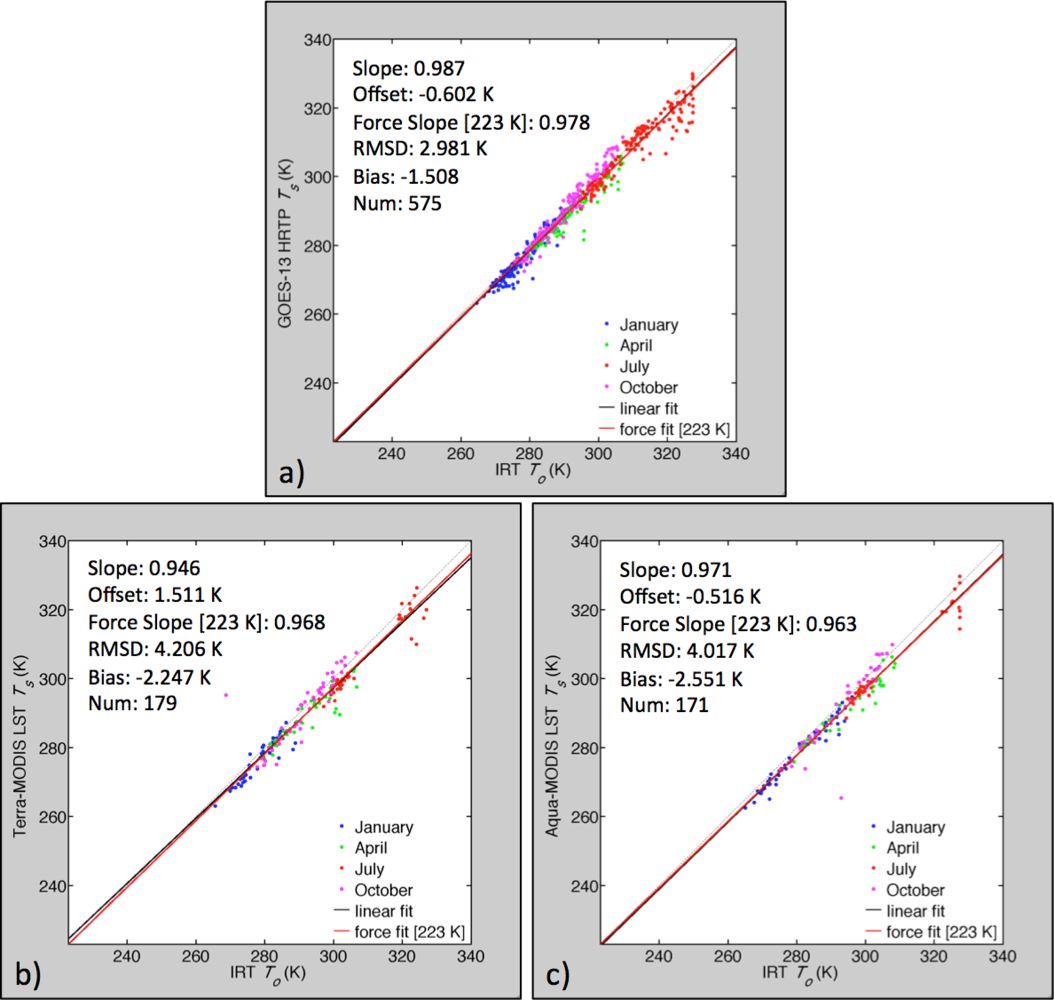
| R2 | 0.97 | 0.96 | 0.99 | 0.95 | 0.95 | 0.98 |
| Bias (K) | −1.5 | −1.5 | 0.6 | −1.1 | −0.1 | 0.4 |
| SDD (K) | 2.6 | 2.8 | 1.4 | 3.4 | 3.4 | 1.8 |
Share and Cite
Scarino, B.; Minnis, P.; Palikonda, R.; Reichle, R.H.; Morstad, D.; Yost, C.; Shan, B.; Liu, Q. Retrieving Clear-Sky Surface Skin Temperature for Numerical Weather Prediction Applications from Geostationary Satellite Data. Remote Sens. 2013, 5, 342-366. https://doi.org/10.3390/rs5010342
Scarino B, Minnis P, Palikonda R, Reichle RH, Morstad D, Yost C, Shan B, Liu Q. Retrieving Clear-Sky Surface Skin Temperature for Numerical Weather Prediction Applications from Geostationary Satellite Data. Remote Sensing. 2013; 5(1):342-366. https://doi.org/10.3390/rs5010342
Chicago/Turabian StyleScarino, Benjamin, Patrick Minnis, Rabindra Palikonda, Rolf H. Reichle, Daniel Morstad, Christopher Yost, Baojuan Shan, and Qing Liu. 2013. "Retrieving Clear-Sky Surface Skin Temperature for Numerical Weather Prediction Applications from Geostationary Satellite Data" Remote Sensing 5, no. 1: 342-366. https://doi.org/10.3390/rs5010342
APA StyleScarino, B., Minnis, P., Palikonda, R., Reichle, R. H., Morstad, D., Yost, C., Shan, B., & Liu, Q. (2013). Retrieving Clear-Sky Surface Skin Temperature for Numerical Weather Prediction Applications from Geostationary Satellite Data. Remote Sensing, 5(1), 342-366. https://doi.org/10.3390/rs5010342