A Hyperspectral Thermal Infrared Imaging Instrument for Natural Resources Applications

Abstract

A new instrument has been setup at the Centre de Recherche Public-Gabriel Lippmann to measure spectral emissivity values of typical earth surface samples in the 8 to 12 μm range at a spectral resolution of up to 0.25 cm⁻¹. The instrument is based on a Hyper-Cam-LW built by Telops with a modified fore-optic for vertical measurements at ground level and a platform for airborne acquisitions. A processing chain has been developed to convert calibrated radiances into emissivity spectra. Repeat measurements taken on samples of sandstone show a high repeatability of the system with a wavelength dependent standard deviation of less than 0.01 (1.25% of the mean emissivity). Evaluation of retrieved emissivity spectra indicates good agreement with reference measurements. The new instrument facilitates the assessment of the spatial variability of emissivity spectra of material surfaces—at present still largely unknown—at various scales from ground and airborne platforms and thus will provide new opportunities in environmental remote sensing.

1. Introduction

Over the last three decades airborne hyperspectral imaging has become a major tool in environmental remote sensing for studying the Earth’s surface and the atmosphere. The 0.35 μm to 2.5 μm spectral range is dominated by reflected sunlight and is well suited for detecting the spectral features related to electronic transitions (e.g., iron oxides, Fe²⁺ bearing minerals, chlorophyll, etc.) and harmonics and combination bands of vibrational absorptions (e.g., OH, SO₄, CO₃, CH, etc.) in minerals, soils, vegetation, and the atmosphere. Thermal infrared (TIR) data provides complementary information in terms of spectral emissivity and temperature of environmental targets, such as key rock and soil forming minerals, specific gaseous components, and vegetation. The 8 μm to 14 μm spectral range spans the radiant energy peak of ambient temperature of the Earth (300 K), whereas the 3 μm to 5 μm band corresponds to the radiant energy peak for hot features (>600 K) such as fires and lava flows according to Wien’s displacement law [1]. Numerous studies have demonstrated the use of TIR data for many thematic areas and applications, for instance landscape characterization, determination of mineral and soil properties [2], estimation of energy fluxes [3] estimation of evapotranspiration and soil moisture, drought monitoring, urban heat islands [4], detection of forest fires, coal fires and volcanoes [5] (compare e.g., [1] and [6] for a comprehensive overview). Currently, TERRA-AQUA/MODIS and other sensors provide low spatial resolution (>1 km) TIR data. Medium spatial resolution TIR data (∼100 m) is provided by TERRA/ASTER and Landsat/TM-ETM+, which will be followed by the Landsat Data Continuity Mission (LDCM, 2 TIR bands, Launch: 2013, http://ldcm.nasa.gov/ [7]) and by the Hyperspectral Infrared Imager (HyspIRI, 7 TIR bands, Launch: 2020, http://hyspiri.jpl.nasa.gov/). High resolution TIR data (∼10 m) is currently only available through on-demand flights in which multispectral or hyperspectral sensors are placed on aircrafts.

Improvements of infrared technology have led to hyperspectral acquisitions in the TIR, i.e., images acquired with hundreds of contiguous spectral channels rather than just 5–10 multispectral channels. While this imaging approach has been used since the 1980s in the visible, near-infrared, and shortwave infrared region, there are presently only a limited number of hyperspectral imaging instruments that operate in the TIR. Hyperspectral TIR instruments operational for airborne surveys, include the thermal emission spectrometer on the Mars Global Surveyor spacecraft [8], the airborne hyperspectral imager (AHI, [9]), the spatially enhanced broadband array spectrograph system (SEBASS, [10]), Itres TASI-600 ( http://www.itres.com/), Specim AisaOWL ( http://www.specim.fi) and the Telops Hyper-Cam [11]. These instruments are dispersive infrared spectrometers, with the exception of the Hyper-Cam that belongs to the class of Fourier transform infrared (FTIR) spectrometers. The main advantage of FTIR-spectrometers over conventional dispersive instruments is their higher achievable signal-to-noise ratio that is based on the following properties [6]: the detector signal in an FTIR-spectrometer contains the contributions of all wavelengths whereas in a conventional dispersive spectrometer the wavelength bands are observed sequentially while scanning the grading. Therefore, in comparable measuring conditions (same detector, measurement time, spectral resolution, optical throughput and optical efficiency) there is in an improved signal-to-noise ratio of FTIR-instruments by N1/2, where N is the number of recorded wavelengths [12]. This is referred to as the Fellgett advantage (also known as the multiplex effect or multiplex advantage). Furthermore, in an interferometer a higher energy throughput and thus, a higher detector signal can be measured. This is known as the Jacquinot advantage (or throughput advantage) and is due to the absence of conventional slits in the interferometer to define the spectral resolution. An additional property of FTIR instruments is their ability for self-calibration. This is achieved by a frequency-stabilized laser (e.g., a HeNe-laser) that is used as an internal wavelength standard and that allows to measure optical path difference of the moving mirror very precisely from the laser interferogram, the so-called Connes advantage.

Clearly, the new hyperspectral thermal infrared instruments require the same level of research for the development of image analysis and processing techniques, field calibration and validation, and new methods for surface characterization, as previous instruments. To date, only a few scientific publications on the calibration and analysis of hyperspectral TIR image data have been published, e.g., da Luz and Crowley [13], Puckrin et al.[14], Vaughan et al.[15]. In this paper we describe a new instrumental setup at the Centre de Recherche Public-Gabriel Lippmann (Belvaux, Luxembourg) with a processing chain to measure spectral emissivity values and surface temperature of typical earth surface samples in the 8 to 12 μm range. Contrary to similar existing instruments, this new design allows for vertical measurements at ground level and airborne acquisitions from an airborne platform.

Accurate interpretation of TIR data requires the separation of temperature and emissivity. The difficulty in the temperature-emissivity separation for multispectral thermal sensors is that the solution equations are underdetermined making it difficult to uniquely separate these two parameters. While in theory this is also under-determined for hyperspectral data, the large number of wavelengths allows a good fit to the Planck radiance for a single temperature [15]. A number of approaches based on different assumptions have been developed to estimate emissivity [16,17], for instance the temperature-emissivity separation algorithm (TES, [16]). However, for agricultural applications the TES procedure tends to underestimate emissivities and consequently overestimate land surface temperatures, with potential emissivity errors of up to 2.0%, resulting in errors of 2–3 °C [18]. Hyperspectral approaches can rely on a large number of wavelengths which allows a good fit to the Planck radiance to determine land surface temperature or canopy temperature at higher accuracies than multispectral procedures [15,19].

Laboratory measurements [20] have shown that TIR emissivity spectra are useful for identifying many minerals [21], rocks, and other solid materials such as plant leaves [22]. However, laboratory spectra commonly do not represent the materials as they would be seen from remote sensing platforms. Besides, the spatial variability of emissivity spectra of material surfaces is largely unknown. Using a hyperspectral TIR imager the emissivity can be examined at various scales depending on platform and sensor viewing geometry [23]. In this paper we will demonstrate in the laboratory that accurate TIR emissivity spectra can be retrieved by the new Hyperspectral TIR Imager.

2. Instrument Setup

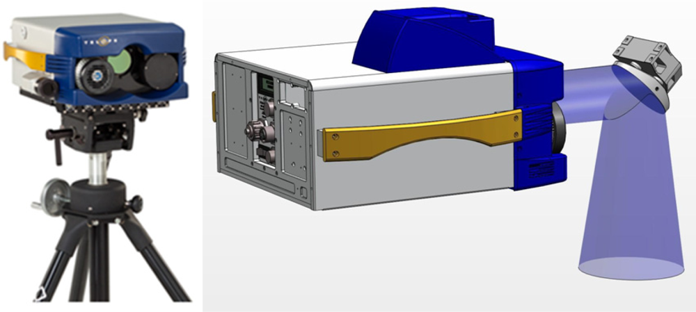
2.1. Base Instrument

The instrument is based on a Hyper-Cam-LW (long wave) [11] built by Telops, Quebec, Canada. The Hyper-Cam-LW is a lightweight and compact imaging radiometric spectrometer. The spectra measurements are performed using an imaging Fourier-transform spectrometer based on a Michelson interferometer coupled to a 320 × 256 long wave infrared photovoltaic MCT (mercury-cadmiumtelluride) focal plane array detector that can be windowed and formatted to fit the desired size. Spectral resolution is user selectable and ranges from 0.25 to 150 cm⁻¹. This instrument gives the complete spectrum of each pixel in the image, each pixel having an instantaneous field-of-view of 0.35 mrad.

The instrument features two internal calibration blackbodies mounted in front of the Hyper-Cam used to perform a complete end-to-end radiometric calibration of the infrared measurements. In its long wave IR version, the instrument has high sensitivity over the 8–12 μm domain. This spectral domain is ideal for passive standoff chemical agent detection at ambient temperatures for which it was originally designed. The sensor also has acquisition and processing electronics, including 4 GB of high-speed DDR-SRAM, with the capability to convert the raw interferograms into radiometrically calibrated spectra using real-time discrete-Fourier transform (DFT). Its weatherproof enclosure provides operability in harsh environments from −10°C to +45°C.

2.2. Modifications: Customized Mirror System, Setup for Vertical Measurements

The Hyper-Cam-LW was modified to allow for vertical (nadir) measurements of targets at the ground level to resemble the observation geometry obtained from airborne or space-borne platforms. The modification consists in a custom designed folding mirror system and a telescope (Figure 1).

The mirror system allows the camera to look downward onto the target by deflecting the upwelling emitted radiation by 90° towards the optical inlet of the Hyper-Cam. The system itself consists of a 45° tilted gold coated mirror that is located in the instrument’s field of view, providing optimal reflectivity in the 8–12 μm spectral range. A 0.25× telescope can be optionally installed to cover a sufficiently large field-of-view (FOV) in the vertical mode. The resulting FOV with the 0.25× telescope at a sensor-target distance of 1.5 m is 672 × 538 mm at a pixel size of 2.1 mm. Without the telescope the FOV is 168 × 134 mm at a pixel size of 0.525 mm.

2.3. Airborne Module

The airborne module includes a stabilization platform, the Image Motion Compensator (IMC) mirror, a GPS/INS (inertial navigation system) unit and a visible boresighted camera. All these modules are rigidly mounted on a high stiffness base plate. This base plate is mounted on the stabilization platform. Figure 2 illustrates the Hyper-Cam airborne configuration.

The IMC mirror is used to compensate the airplane pitch, roll and forward motion while the stabilization platform is used to dampen the airplane vibrations and to compensate the airplane yaw. The IMC mirror is controlled by the navigation module which receives and uses the information from the video tracker and the GPS/INS unit which enables ortho-rectification and geo-referencing of the collected data. The Hyper-Cam instrument offers uncommon flexibility in adjusting its spatial, spectral and temporal parameters. This flexibility proves to be invaluable for airborne applications where the flight parameters impose severe restrictions on spectrometer operation.

3. Measurement Procedures

To illustrate the capabilities of the system, measurements were done in the laboratory using heated rock and mineral samples. In this way it was possible to avoid poor outside weather conditions and to ensure stable conditions during measurements.

3.1. Instrument Preparation and Settings

To setup the system for measurements, the Hyper-Cam was mounted on its tripod and the connections were plugged for CameraLink, Firewire (IEEE1394), RJ45 Ethernet and power. The start-up sequence consists of switching on the sensor, waiting for the internal diagnostics, launching the internal software suite Reveal Pro and waiting for the focal plane arrays (FPA) to cool down to 120 K which usually takes less than two minutes.

3.2. Sample Preparation

The primary sample used in this study, i.e., for testing the repeatability and the emissivity retrieval and for inspecting spatial emissivity features was a sandstone rock sample from the Lower Trias (Buntsandstein or Bunter Sandstone). The emissivity retrieval was repeated with quartz and calcite crystals. To obtain a high contrast between the sample and the surroundings in the laboratory, the sample was heated up to about 30 K above ambient temperature using an oven. The exact sample temperature was measured with a contact thermometer. The sample was placed at 3 m distance from the sensor so that the measured surface was perpendicular to the optical axis of the camera.

3.3. Instrument Calibration

The instrument’s spectral response is dependent on several factors such as detector responsivity, coatings, channel settings and integration time. A radiometric calibration is needed to acquire calibrated spectra in units of radiance [17]. Assuming linearity of FTIR spectrometers, the spectral response and the non-uniformities are determined for every pixel and the non-uniformities are eliminated during the calibration process using a 2-point complex radiometric calibration. For calibration, images of hot and cold blackbodies are acquired. The blackbodies’ temperature can be controlled very accurately (<0.03 K stability) from ambient −15 K to ambient +75 K and should be chosen so that blackbodies are framing the scene’s emitted radiation.

In this experiment, cold and hot blackbody temperatures were set to 15 °C and 65 °C, respectively, and the ambient temperature was 22 °C. Knowing the blackbodies’ temperature as well as their exact spectral emissivity values, their spectral radiance was determined using the Planck’s function. Starting from these two blackbody frames, a gain and offset function was calculated for every pixel which was then applied to the scene’s raw spectra resulting in calibrated radiance spectra (Figure 3).

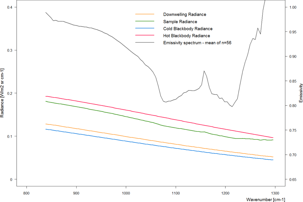
3.4. Background Radiation

Reflected or emitted radiance from background objects, i.e., the walls and ceiling in the laboratory significantly contribute to the target measurement [24]. The background radiation (downwelling radiance) was measured immediately following the sample measurement by collecting the radiance of a diffuse reflective aluminum plate. The aluminum plate’s exact temperature (ambient) was measured using a contact thermometer. The (unknown) emissivity of the aluminum plate was determined relative to an infragold target with known emissivity. This measurement was performed by a Bruker Vertex 70 FTIR spectrometer. The resulting overall emissivity value was 20% which is in good agreement with values found in literature.

3.5. Emissivity Calculation

Emissivity is a sample’s efficiency to behave as a blackbody radiator and is scaled between 0 and 1. The calculation of a sample’s emissivity requires knowledge of the radiance spectrum of a blackbody with the sample’s temperature. However, accurate determination of the (unknown) sample temperature is often difficult and requires fitting the Planck equation to a measured radiance spectrum. Hyperspectral data with its continuous coverage of wavebands allows a good fit to the Planck radiance curve for spectral regions where emissivity is close to unity [15].

Emissivity was assumed to have a certain fixed value over a defined wavelength region which allowed to iteratively fit a Planck radiance curve to the measured sample radiance spectrum. Emissivity was set to a value of 0.97 at the wavelength of the maximum brightness temperature following the approach by Kealy and Hook [25]. The fitting was performed over wavebands from 850 to 905 wavenumbers. An alternative approach would have been to set emissivity to a value of 1.0 in the 7.7–7.8 μm region. In this region where silicate minerals typically have their Christiansen frequency, the emissivity is generally assumed constant and very close to 1.0 [17]. However, the first approach was preferred, as it produced more realistic emissivity spectra.

Blackbody radiance was simulated in unit wavenumber σ, commonly used in spectroscopy as ( http://www.spectralcalc.com/):

$${L\_bb}_{\sigma }\left(T\right)=2{hc}^2{\sigma }^3\frac{1}{e^{\frac{hc\sigma }{kT}}-1}{Wm}^{-2}s{r}^{-1}{\left(c{m}^{-1}\right)}^{-1}$$

where L_bb_σ is the spectral radiance emitted by a blackbody at the absolute temperature T for wavenumber σ, h is the Planck constant, k is the Boltzmann constant, and c is the speed of light.

The blackbody radiance was then fitted to the measured sample radiance L_sa_σ over the defined waveband region by adjusting T assuming the predefined emissivity ε_σ:

$${L\_sa}_{\sigma }={\epsilon }_{\sigma }{L\_bb}_{\sigma }\left(T\right)$$

Finally, spectral emissivity ε_σ was calculated as:

$${\epsilon }_{\sigma }=\frac{{L\_sa}_{\sigma }-{L\_dw}_{\sigma }}{{L\_bb}_{\sigma }\left(T\right)-{L\_dw}_{\sigma }}$$

where L_dw_σ is the downwelling radiance. L_dw_σ was determined following an approach by Horton and co-workers [26]:

$${L\_dw}_{\sigma }=\frac{{L\_\mathit{ref}}_{\sigma }-{\epsilon }_{{\mathit{ref}}_{\sigma }}\cdot {L\_BB}_{\sigma ,T}}{1-{\epsilon }_{{\mathit{ref}}_{\sigma }}}$$

where L_refσ = measured radiance from reference panel (aluminum or infragold), ε_refσ = spectral emissivity of reference panel, L_BB_σT = blackbody radiance at temperature T of reference panel.

3.6. Testing Repeatability

For testing repeatability of data measured with the Hyper-Cam replicate measurements of the same sample material were performed under laboratory conditions. An experimental setup was chosen to allow acquiring multiple data cubes in a short time interval. To have a limited cooling effect on the recorded spectra, small image subsets (64 × 20 pixels) were acquired at a spectral resolution of 6.2 cm⁻¹. The sandstone sample was placed at a distance of three meters from the sensor. The sandstone sample was uniformly heated up to 60 °C and 20 frames were captured within 30 s. During this short time interval the temperature of the sample decreased less than 0.5 K as measured with a contact thermometer. This image acquisition was repeated thrice so that altogether 58 frames were measured (two frames were removed). Due to the direct dependence of the radiance spectra on the sample temperature; emissivity spectra (temperature independent) were derived and considered for further investigation. Downwelling radiation was corrected for by measuring a diffuse reflecting aluminum plate.

In a user defined region of interest, the radiance spectra were isolated for every pixel and the mean emissivity spectrum was derived. Using the n = 58 emissivity spectra, for every single wavenumber the mean value x̄ and standard deviation s were computed and the confidence interval was calculated as $\overline{x}\pm s\left(t/\sqrt{n}\right)$, where t is a critical value determined from the t_n−1 distribution.

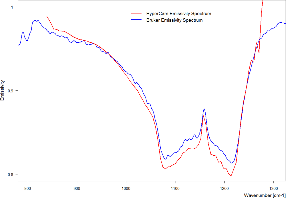
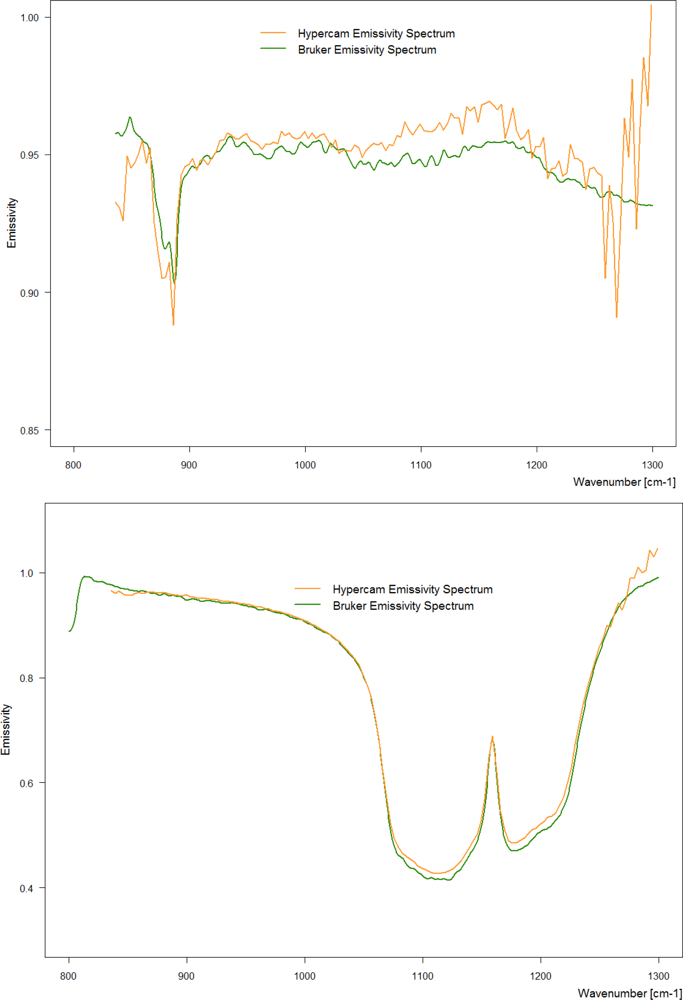
3.7. Comparison with Reference Spectra

Derived emissivity spectra were compared with reference spectra. The same rock and mineral samples were measured at the spectrometry laboratory of University of Twente (ITC) using a laboratory device (Bruker Vertex 70 FTIR spectrometer) following the procedures described in [20]. The spectra were measured in directional hemispherical reflectance. Assuming opaque properties of the rock samples, the emissivity was obtained by using Kirchhoff’s Law (ε = 1 − ρ) which previously had been verified by both laboratory and field measurements [24,27]. In addition, sandstone emissivity spectra from a spectral library collected by John Hopkins University were used for a plausibility check.

4. Results and Discussion

4.1. Repeatability

To test the repeatability of the system, replicate measurements of the sandstone sample were analyzed. A plot of the mean emissivity spectrum and the standard deviation of 58 single measurements (Figure 4) indicate good repeatability over the three measurement cycles with standard deviations less than 0.01 and variation coefficients of up to 1.25%.

Hecker [20] performed a repeatability test for absolute measurements of directional-hemispherical reflectance (DHR) of quartz sand over 2 weeks using a Bruker Vertex 70 FTIR spectrometer. They obtained standard deviations in the range of 0.001 to 0.007 for most wavelengths which corresponds, with a mean DHR value of 0.4 at 9 μm, to variation coefficients of 0.25%–1.75%. In comparison to these values, a variation coefficient of up to 1.25% obtained with the Hyper-Cam-LW seems to be acceptable.

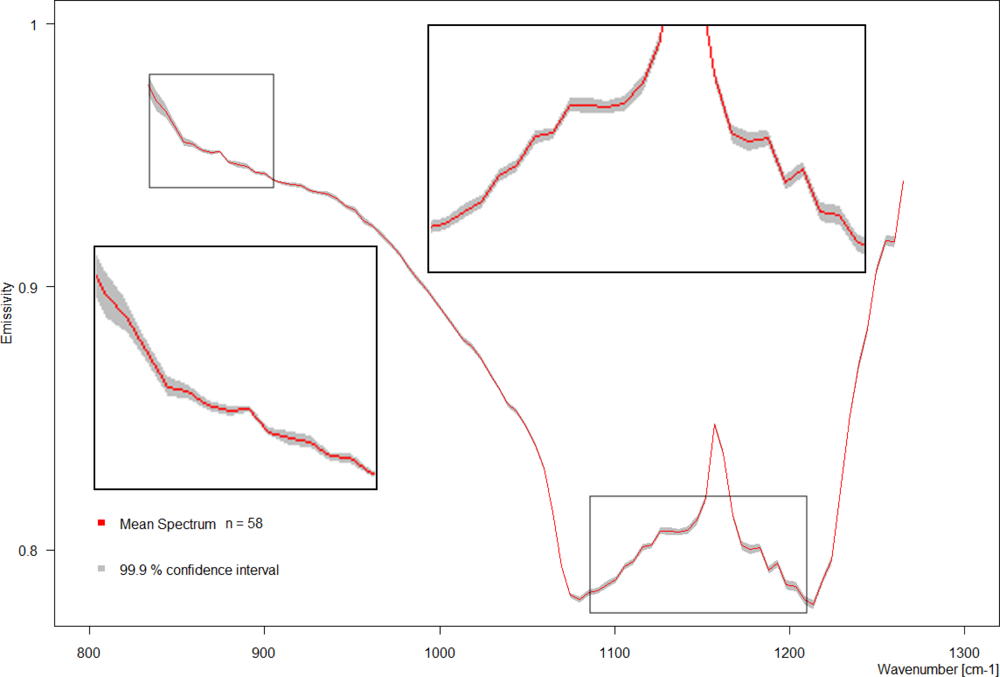
4.2. Comparison of Emissivity Spectra with Reference Spectra

The comparison of the Bunter Sandstone emissivity spectrum derived with the Hyper-Cam-LW and the Bruker Vertex 70 (Figure 5) shows a relatively good agreement. Both spectra show the main quartz doublet around 1,175 cm⁻¹ with the characteristic maximum and the minima around 1,080 cm⁻¹ and around 1,220 cm⁻¹. The spectra agree particularly well for the spectral regions left and right of the Quartz doublet. However, for wavenumbers between the two minima larger discrepancies between Hyper-Cam and Bruker spectra exist. One explanation for this difference is that different parts of the sandstone sample were observed during the two measurement setups. Besides, the comparison of the Bunter Sandstone emissivity spectrum derived with the Hyper-Cam-LW with two sandstone spectra (Arkosic Sandstone and Ferruginous Sandstone) of the spectral library of John Hopkins University indicated a general agreement in the shape of the curves (not shown). Also the other Hyper-Cam emissivity spectra obtained for calcite and quartz (Figure 6) compare relatively well to the Bruker reference spectra with respect to their main spectral features. In comparison to previously published spectra, e.g., [17], the quartz spectrum reveals similarities in the general shape of the spectrum, but also differences in the magnitude of emissivity, i.e., at 1,220 cm⁻¹ε∼0.80 in this study and ε∼0.60 in [17]. These enormous differences are likely to be caused by differences in surface roughness. For instance, differences in emissivity of comparable magnitude (e.g., ε-differences of up to 0.25) were also found by [23] for matte and rough mineral samples of identical mineral composition.

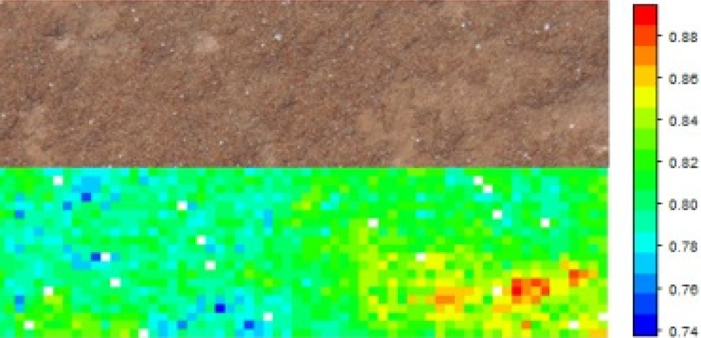
4.3. Spatial Variability of Emissivity

When looking at the spatial emissivity patterns (Figure 7), there is a clear variation of emissivity over the sandstone surface which is not obvious from a visual inspection of the rock sample. Within the dominant matrix of emissivity values of 0.81–0.83 (shown in green colour) there are marked areas with much smaller values of around 0.76–0.78 (shown in blue) and larger values of around 0.86–0.88 (shown in red). The observed spectral emissivity variations within the rock sample may be attributed to roughness, surface geometry, and compositional variation [23].

5. Conclusions and Outlook

The first tests with the new Hyperspectral Thermal Infrared Imaging Instrument suggest that the system is capable of measuring spectral emissivity and its spatial variation over natural surfaces with good accuracy. Current tests were performed in the laboratory with heated rock samples and will be repeated outside under clear sky conditions with samples at ambient temperature.

The similarity between the emissivity spectra obtained by the Hyper-Cam and reference spectra (Bruker Vertex 70 and JHU spectral library) appears close enough for mapping such minerals from airborne hyperspectral (or spaceborne multispectral) TIR measurements (such as ASTER Level 2 surface emissivity products) based on the shapes of the laboratory reference spectra, for instance using respective band ratio techniques [28].

The final implementation of the airborne platform will facilitate generating accurate maps of land surface emissivity and land surface temperature at very high spatial resolution which in turn will provide new opportunities in environmental remote sensing such as monitoring natural and urban environments, volatile organic compounds, detection of vegetation stress, evapotranspiration rates and energy fluxes, mineral mapping, and bio-diversity.

Airborne observations require taking atmospheric effects and instrument noise into consideration [29]. Since atmospheric absorption (mainly by H₂O and CO₂) is the dominant process in the TIR, while dispersion processes are negligible, at a first glance atmospheric correction in the TIR seems to be simpler than for shortwave radiation. However, it has to be noted that in addition to the surface, the atmosphere also emits radiation towards the sensor. This requires solving the equation of radiative transfer for the TIR region, which makes the interpretation of airborne hyperspectral TIR data more ambiguous than ground based measurements.

Due to the complementary nature of the reflective (VSWIR) and emissive (TIR) spectral regions a synergistic use of airborne data from both domains bears great potential. This might significantly improve our understanding of biochemical and physical land surface properties. Specifically, VSWIR imaging spectrometers can discriminate surface materials and TIR data acquisitions can help to identify thermal characteristics for different material and land cover types. For instance, combining emissivity spectra with reflectance spectra in a mixing model would improve discriminating soils from impervious surfaces [30].

References

1. Jensen, J.R. Remote Sensing of the Environment: An Earth Resource Perspective, 2nd ed.; Pearson Prentice Hall: Upper Saddle River, NJ, USA, 2007; p. 592. [Google Scholar]
2. Eisele, A.; Lau, I.; Hewson, R.; Carter, D.; Wheaton, B.; Ong, C.; Cudahy, T.J.; Chabrillat, S.; Kaufmann, H. Applicability of the thermal infrared spectral region for the prediction of soil properties across semi-arid agricultural landscapes. Remote Sens 2012, 4, 3265–3286. [Google Scholar]
3. Frey, C.M.; Parlow, E. Flux measurements in Cairo. Part 2: On the determination of the spatial radiation and energy balance using ASTER satellite data. Remote Sens 2012, 4, 2635–2660. [Google Scholar]
4. Ogashawara, I.; Bastos, V.S.B. A quantitative approach for analysing the relationship between urban heat islands and land cover. Remote Sens 2012, 4, 3596–3618. [Google Scholar]
5. Carter, A.; Ramsey, M. Long-term volcanic activity at Shiveluch Volcano: Nine years of ASTER spaceborne thermal infrared observations. Remote Sens 2010, 2, 2571–2583. [Google Scholar]
6. Vollmer, M; Möllmann, K.-P. Infrared Thermal Imaging: Fundamentals, Research and Applications; Wiley-VCH: Weinheim, Germany, 2010. [Google Scholar]
7. Schott, J.; Gerace, A.; Brown, S.; Gartley, M.; Montanaro, M.; Reurer, D.C. Simulation of image performance characteristics of the Landsat Data Continuity Mission (LDCM) Thermal Infrared Sensor (TIRS). Remote Sens 2012, 4, 2477–2491. [Google Scholar]
8. Christensen, P.R.; Bandfield, J.L.; Hamilton, V.E.; Ruff, S.W.; Kieffer, H.H.; Titus, T.N.; Greenfield, M. Mars global surveyor thermal emission spectrometer experiment: Investigation description and surface science results. J. Geophys. Res 2001. [Google Scholar] [CrossRef]
9. Lucey, P.G.; Williams, T.J.; Hinrichs, J.L.; Winter, M.E.; Steutel, D.; Winter, E.M. Three years of operation of AHI: The University of Hawaii’s airborne hyperspectral imager. Proc. SPIE 2001. [Google Scholar] [CrossRef]
10. Hackwell, J.A.; Warren, D.W.; Bongiovi, R.P.; Hansel, S.J.; Hayhurst, T.L.; Mabry, D.J.; Sivjee, M.G.; Skinner, J.W. LWIR/MWIR imaging hyperspectral sensor for airborne and ground-based remote sensing. Proc. SPIE 1996, 2819, 102–107. [Google Scholar]
11. Lagueux, P.; Farley, V.; Rolland, M.; Chamberland, M.; Puckrin, E.; Turcotte, C.S.; Lahaie, P.; Dube, D. Airborne Measurements in the Infrared Using FTIR-Based Imaging Hyperspectral Sensors. Proceedings of First Workshop on Hyperspectral Image and Signal Processing: Evolution in Remote Sensing, Grenoble, France, 26–28 August 2009; pp. 482–485.
12. Hirschfeld, T. Wavenumber scale shift in Fourier transform infrared spectrometers due to vignetting. Appl. Spectrosc 1976, 30, 549–550. [Google Scholar]
13. Da Luz, B.R.; Crowley, J.K. Identification of plant species by using high spatial and spectral resolution thermal infrared (8.0–13.5 μm) imagery. Remote Sens. Environ 2010, 114, 404–413. [Google Scholar]
14. Puckrin, E.; Turcotte, C.S.; Lahaie, P.; Dube, D.; Farley, V.; Lagueux, P.; Marcotte, F.; Chamberland, M. Airborne infrared-hyperspectral mapping for detection of gaseous and solid targets. Proc. SPIE 2012. [Google Scholar] [CrossRef]
15. Vaughan, R.G.; Calvin, W.M.; Taranik, J.V. SEBASS hyperspectral thermal infrared data: Surface emissivity measurement and mineral mapping. Remote Sens. Environ 2003, 85, 48–63. [Google Scholar]
16. Gillespie, A.; Rokugawa, S.; Matsunaga, T.; Cothern, J.S.; Hook, S.; Kahle, A.B. A temperature and emissivity separation algorithm for Advanced Spaceborne Thermal Emission and Reflection Radiometer (ASTER) images. IEEE Trans. Geosci. Remote Sens 1998, 36, 1113–1126. [Google Scholar]
17. Hook, S.J.; Kahle, A.B. The micro Fourier Transform Interferometer (mu FTIR)—A new field spectrometer for acquisition of infrared data of natural surfaces. Remote Sens. Environ 1996, 56, 172–181. [Google Scholar]
18. French, A.N.; Schmugge, T.J.; Ritchie, J.C.; Hsu, A.; Jacob, F.; Ogawa, K. Detecting land cover change at the Jornada Experimental Range, New Mexico with ASTER emissivities. Remote Sens. Environ 2008, 112, 1730–1748. [Google Scholar]
19. Da Luz, B.R.; Crowley, J.K. Spectral reflectance and emissivity features of broad leaf plants: Prospects for remote sensing in the thermal infrared (8.0–14.0 μm). Remote Sens. Environ 2007, 109, 393–405. [Google Scholar]
20. Hecker, C.; Hook, S.; van der Meijde, M.; Bakker, W.; van der Werff, H.; Wilbrink, H.; van Ruitenbeek, F.; de Smeth, B.; van der Meer, F. Thermal infrared spectrometer for earth science remote sensing applications-instrument modifications and measurement procedures. Sensors 2011, 11, 10981–10999. [Google Scholar]
21. Salisbury, J.; Walter, L.; Vergo, N.; D’Aria, D. Infrared (2.1–25 Micrometers) Spectra of Minerals; The Johns Hopkins University Press: Baltimore, MD, USA, 1992. [Google Scholar]
22. Ullah, S.; Schlerf, M.; Skidmore, A.K.; Hecker, C.A. Identifying plant species using mid-wave infrared, 2.5–6 μm, and thermal infrared, 8–14 μm, emissivity spectra. Remote Sens. Environ 2012, 118, 95–102. [Google Scholar]
23. Balick, L.; Gillespie, A.; French, A.; Danilina, I.; Allard, J.P.; Mushkin, A. Longwave thermal infrared spectral variability in individual rocks. IEEE Geosci. Remote Sens. Lett 2009, 6, 52–56. [Google Scholar]
24. Korb, A.R.; Dybwad, P.; Wadsworth, W.; Salisbury, J.W. Portable Fourier transform infrared spectroradiometer for field measurements of radiance and emissivity. Appl. Opt 1996, 35, 1679–1692. [Google Scholar]
25. Kealy, P.S.; Hook, S.J. Separating temperature and emissivity in thermal infrared multispectral scanner data: Implications for recovery of land surface temperatures. IEEE Trans. Geosci. Remote Sens 1993, 31, 1155–1164. [Google Scholar]
26. Horton, K.A.; Johnson, J.R.; Lucey, P.G. Infrared measurements of pristine and disturbed soils 2. Environmental effects and field data reduction. Remote Sens. Environ 1998, 64, 47–52. [Google Scholar]
27. Salisbury, J.W.; Wald, A.; D’Aria, D.M. Thermal-infrared remote sensing and Kirchhoff’s law: 1. Laboratory measurements. J. Geophys. Res 1994, 99, 897–911. [Google Scholar]
28. Rockwell, B.W.; Hofstra, A.H. Identification of quartz and carbonate minerals across northern Nevada using ASTER thermal infrared emissivity data—Implications for geologic mapping and mineral resource investigations in well-studied and frontier areas. Geosphere 2008, 4, 218–246. [Google Scholar]
29. Jimenez-Munoz, J.C.; Sobrino, J.A.; Gillespie, A.R. Surface emissivity retrieval from airborne hyperspectral scanner data: Insights on atmospheric correction and noise removal. IEEE Geosci. Remote Sens. Lett 2012, 9, 180–184. [Google Scholar]
30. Roberts, D.A.; Quattrochi, D.A.; Hulley, G.C.; Hook, S.J.; Green, R.O. Synergies between VSWIR and TIR data for the urban environment: An evaluation of the potential for the Hyperspectral Infrared Imager (HyspIRI) Decadal Survey mission. Remote Sens. Environ 2012, 117, 83–101. [Google Scholar]
Figure 1. Hyper-Cam-LW Sensor (left) and instrument setup for ground measurements (right).
Remotesensing 04 03995f1
Figure 2. Hyper-Cam airborne assembly (top) and acquisition scheme (bottom): The IMC system is servo controlled to ensure the sensor is staring at a fixed scene during the acquisition of the hyperspectral image.
Remotesensing 04 03995f2
Figure 3. Measurement sequence of sample (sandstone), cold blackbody, hot blackbody and downwelling radiation and the derived sample emissivity spectrum. The lines shown represent the mean of 56 single measurements.
Remotesensing 04 03995f3
Figure 4. Demonstration of repeatability: The red line is an average of 56 single measurements and the grey band indicates the 99.9% confidence interval of the mean at each wavenumber.
Remotesensing 04 03995f4
Figure 5. Emissivity spectra of the Bunter Sandstone sample derived from the Hyper-Cam (red) and from the Bruker (blue).
Remotesensing 04 03995f5
Figure 6. Emissivity spectra of Calcite (top), and Quartz (bottom) derived from Hyper-Cam and Bruker spectrometers.
Remotesensing 04 03995f6
Figure 7. Surface of the sandstone sample (top) and derived emissivity values at 1,095 cm−1 (bottom). White pixels are detector failures which are marked as bad pixels by the Reveal Pro software.
Remotesensing 04 03995f7