Cost-Effectiveness of Seven Approaches to Map Vegetation Communities — A Case Study from Northern Australia’s Tropical Savannas


Abstract
:1. Introduction
2. Data and Methods
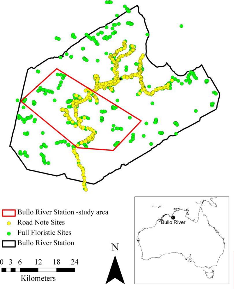
2.1. Study Area
2.2. Field Data Sampling
2.3. Field Data Analysis and Vegetation Community Classification
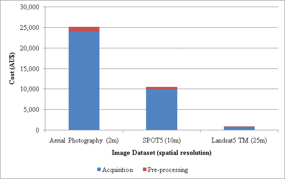
2.4. Image Data Acquisition and Pre-Processing
2.5. Training Areas and Ancillary Data
2.6. Classification Methods
2.6.1. Aerial Photography Interpretation
2.6.2. Pixel-Based Image Analysis
2.6.3. Object-Based Image Analysis
- an image-only NN classification (image data and training areas),
- an integrated NN classification (image and ancillary data and training areas)
- an image-only step-wise classification (image data),
- an integrated step-wise classification (image and ancillary data).
Segmentation
Nearest Neighbor Classifications
Image-only Step-Wise Classification
Integrated Step-Wise Classification
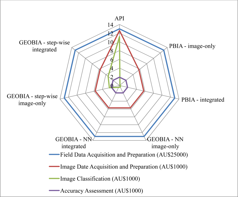
2.7. Cost-Effectiveness
3. Results and Discussion
3.1. Vegetation Communities
3.2. Cost-Effectiveness
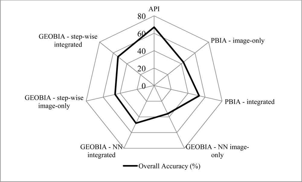
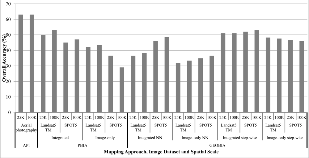
3.2.1. Accuracy Assessment
3.2.2. Cost
- API: 1:50,000 aerial photography mosaic at 1:100,000,
- PBIA image-only: Landsat5 TM at 1:100,000,
- PBIA integrated: Landsat5 TM (DEM and slope) at 1:100,000,
- GEOBIA NN image-only: SPOT5 at 1:100,000,
- GEOBIA NN integrated: SPOT5 (DEM and slope) at 1:100,000,
- GEOBIA step-wise image-only: SPOT5 (contextual information) at 1:100,000, and
- GEOBIA step-wise integrated: SPOT5 (DEM, slope and contextual information) at 1:100,000.
4. Conclusions
Acknowledgments
References
- Thackway, R.; Lee, A.; Donohue, R.; Keenan, R.J.; Wood, M. Vegetation information for improved natural resource management in Australia. Landsc. Urban Plan 2007, 79, 127–136. [Google Scholar]
- Weiers, S.; Bock, M.; Wissen, M.; Godela, R. Mapping and indicator approaches for the assessment of habitats at different scales using remote sensing and GIS methods. Landsc. Urban Plan 2004, 67, 43–65. [Google Scholar]
- Kerr, J.; Ostrovsky, M. From space to species: Ecological applications for remote sensing. Trends Ecol. Evol 2003, 18, 299–305. [Google Scholar]
- Wulder, M.A.; Franklin, S.E. Remote Sensing of Forest Environments: Concepts and Case Studies; Kluwer Academic Publishers: Norwell, MA, USA, 2003. [Google Scholar]
- Franklin, S.E. Remote Sensing for Sustainable Forest Management; Lewis Publishers, CRC Press LLC: Boca Raton, FL, USA, 2001. [Google Scholar]
- Mehner, H.; Cutler, M.; Fairbairn, D.; Thompson, G. Remote sensing of upland vegetation: the potential of high spatial resolution satellite sensors. Glob. Ecol. Biogeogr 2004, 13, 359–369. [Google Scholar]
- Lees, B.G.; Ritman, K. Decision-tree and rule-induction approach to integration of remotely sensed and GIS data in mapping vegetation in disturbed or hilly environments. Environ. Manage 1991, 15, 823–831. [Google Scholar]
- Lu, D.; Weng, Q. A survey of image classification methods and techniques for improving classification performance. Int. J. Remote Sens 2007, 28, 823–870. [Google Scholar]
- Miller, J.; Franklin, J.; Aspinall, R. Incorporating spatial dependence in predictive vegetation models. Ecol. Model 2007, 202, 225–242. [Google Scholar]
- Goetz, S.J.; Wright, R.K.; Smith, A.J.; Zinecker, E.; Schaub, E. IKONOS imagery for resource management: Tree cover, impervious surfaces, and riparian buffer analyses in the mid-Atlantic region. Remote Sens. Environ 2003, 88, 195–208. [Google Scholar]
- Koch, B.; Ivitis, E.; Jochum, M. Forest classification with eCognition and ERDAS expert classifier: Object-based versus Pixel-based. GIM Int 2003, 17, 12–15. [Google Scholar]
- Flanders, D.; Hall-Beyer, M.; Pereverzoff, J. Preliminary evaluation of eCognition object-based software for cut block delineation and feature extraction. Can. J. Remote Sens 2003, 29, 441–452. [Google Scholar]
- Laliberte, A.; Fredrickson, E.; Rango, A. Combining decision trees with hierarchical object-oriented image analysis for mapping arid rangelands. Photogramm. Eng. Remote Sensing 2007, 73, 197–207. [Google Scholar]
- Ivits, E.; Koch, B.; Blaschke, T.; Waser, L. Landscape Connectivity Studies on Segmentation Based Classification and Manual Interpretation of Remote Sensing Data. Proceedings of eCognition User Meeting, Munich, Germany, 28–30 October 2002.
- Wang, L.; Sousa, W.P.; Gong, P. Integration of object-based and pixel-based classification for mapping mangroves with IKONOS imagery. Int. J. Remote Sens 2004, 25, 5655–5668. [Google Scholar]
- Gibbes, C.; Adhikari, S.; Rostant, L.; Southworth, J.; Qiu, Y. Application of object based classification and high resolution satellite imagery for savannah ecosystem analysis. Remote Sens 2010, 2, 2748–2772. [Google Scholar]
- Mumby, P.; Edwards, A. Mapping marine environments with IKONOS imagery: Enhanced spatial resolution can deliver greater thematic accuracy. Remote Sens. Environ 2002, 82, 248–257. [Google Scholar]
- Stickler, C.; Southworth, J. Application of multi-scale spatial and spectral analysis for predicting primate occurance and habitat associations in Kibale National Park, Uganda. Remote Sens. Environ 2008, 112, 2170–2186. [Google Scholar]
- Gould, W. Remote sensing of vegetation, plant species richness, and regional biodiversity hotspots. Ecol. Appl 2000, 10, 1861–1870. [Google Scholar]
- Lewis, M. Species composition related to spectral classification in an Australian spinifex hummock grassland. Int. J. Remote Sens 1994, 15, 3223–3239. [Google Scholar]
- Lewis, M. Numeric classification as an aid to spectral mapping of vegetation communities. Plant Ecol 1998, 136, 133–149. [Google Scholar]
- Ozesmi, S.; Bauer, M. Satellite remote sensing of wetlands. Wetlands Ecol. Manage 2002, 10, 381–402. [Google Scholar]
- Richards, J.; Landgrebe, D.; Swain, P. A means of utlising ancillary information in multispectral classification. Remote Sens. Environ 1982, 12, 463–477. [Google Scholar]
- Tunstall, B.; Harrison, B.; Jupp, D. Incorporation of Geographical Data in the Analysis of Landsat Imagery for Land-Use Mapping—A Case Example. Proceedings of Australasian Remote Sensing Conference, Adelaide, Australia, August 1987.
- Rogan, J.; Franklin, J.; Roberts, D. A comparison of methods for monitoring multitemporal vegetation change using Thematic Mapper imagery. Remote Sens. Environ 2002, 80, 143–156. [Google Scholar]
- Howe, D. Personal Communication. 2006.
- Wilson, B. Personal Communication. 2006.
- Mumby, P.J.; Green, E.P.; Edwards, A.J.; Clark, C.D. The cost-effectiveness of remote sensing for tropical coastal resources assessment and management. J. Environ. Manage 1999, 55, 157–166. [Google Scholar]
- Malthus, T.J.; Mumby, P.J. Remote sensing of the coastal zone: An overview and priorities for future research. Int. J. Remote Sens. 2003, 24, 2805–2815. [Google Scholar]
- Phinn, S.R.; Stow, D.A.; Franklin, J.; Mertes, L.A.K.; Michaelsen, J. Remotely sensed data for ecosystem analyses: Combining hierarchy theory and scene models. Environ. Manage 2003, 31, 429–441. [Google Scholar]
- Green, E.P.; Mumby, P.J.; Edwards, A.J.; Clark, C.D. Remote Sensing Handbook for Tropical Coastal Management; UNESCO: Paris, France, 2000. [Google Scholar]
- Stehman, S.V. Selecting and interpreting measures of thematic classification accuracy. Remote Sens. Environ 1997, 62, 77–89. [Google Scholar]
- Foody, G.M. Status of land cover classification accuracy assessment. Remote Sens. Environ 2002, 80, 185–201. [Google Scholar]
- Jensen, J.R. Introductory Digital Image Processing: A Remote Sensing Perspective; Prentice Hall: Upper Saddle River, NJ, USA, 2005. [Google Scholar]
- Congalton, R.G. A review of assessing the accuracy of classifications of remotely sensed data. Remote Sens. Environ 1991, 37, 35–46. [Google Scholar]
- Pontius, R.G.; Millones, M. Death to Kappa: birth of quantity disagreement and allocation disagreement for accuracy assessment. Int. J. Remote Sens 2012, 32, 4407–4429. [Google Scholar]
- Foody, G.M. Classification accuracy assessment. IEEE Geosci. Remote Sens. Soc. Newsl. 2011, 8–14. [Google Scholar]
- Wulder, M. Optical remote-sensing techniques for the assessment of forest inventory and biophysical parameters. Progr. Phys. Geogr 1998, 22, 449–476. [Google Scholar]
- de Bruin, S.; Hunter, G.J. Making the trade-off between decision quality and information cost. Photogramm. Eng. Remote Sensing 2003, 69, 91–98. [Google Scholar]
- Lewis, D.; Hill, J.; Cowie, I.D. Bullo River Station Flora and Vegetation Survey, Northern Territory: and Reconnaissance Soil-Landscape Investigation; Technical Report No. 02/2010D; Department of Natural Resources, Environment, The Arts and Sport, Northern Territory Government: Palmerston, NT, Australia, 2010. [Google Scholar]
- Hnatiuk, K.; Thackway, R.; Walker, J. Vegetation. In Australian Soil and Land Survey: Field Handbook; CSIRO Publishing: Collingwood, VIC, Australia, 2008; p. 111. [Google Scholar]
- ESCAVI. Australian Vegetation Attribute Manual: National Vegetation Information System; Version 6.0.; Executive Steering Committee for Australian Vegetation Information, Department of the Environment and Heritage: Canberra, Australia, 2003. [Google Scholar]
- Lewis, D.; Phinn, S. Accuracy assessment of vegetation community maps generated by aerial photography interpretation: Perspective from the tropical savanna, Australia. J. Appl. Remote Sens. 2011. [Google Scholar] [CrossRef] [Green Version]
- Tickell, S.J.; Rajaratnam, L.R. Water Resources Survey of the Western Victoria River District, Bullo River Station; Power and Water Authority, Water Resources Division, Northern Territory Government: Darwin, NT, Australia, 1995. [Google Scholar]
- Curran, P.J. Classification. In Principles of Remote Sensing; Longman: London, UK, 1985; pp. 209–216. [Google Scholar]
- Green, E; Clark, C; Mumby, P; Edwards, A; Ellis, A. Remote sensing techniques for mangrove mapping. Int. J. Remote Sens 1998, 5, 935–956. [Google Scholar]
- Lillesand, T; Kiefer, R. Remote Sensing and Image Interpretation; John Wiley and Sons Inc: New York, NY, USA, 1994. [Google Scholar]
- Mather, P. Computer Processing of Remotely Sensed Images: An Introduction; John Wiley and Sons Ltd: West Sussex, UK, 1999. [Google Scholar]
- Lewis, D.; Phinn, S.; Pfitzner, K. Pixel-based image classification to map vegetation communities using SPOT5 and Landsat5 Thematic Mapper data in a tropical savanna, northern Australia. Can. J. Remote Sens. 2012; accepted. [Google Scholar]
- Lewis, D.; Phinn, S.; Arroyo, L. Object-based image analysis to map vegetation communities using SPOT5, Landsat5 TM, field and ancillary data in a tropical savanna, northern Australia. Int. J. Remote Sens. 2012; accepted. [Google Scholar]
- Salehi, B.; Zhang, Y.; Zhong, M.; Vivek, D. Object-based classification of urban areas using VHR imagery and height points ancillary data. Remote Sens 2012, 4, 2256–2276. [Google Scholar]
- Bahadur, K. Improving Landsat and IRS image classification: evaluation of unsupervised and supervised classification through band ratios and DEM in a mountainous landscape in Nepal. Remote Sens 2009, 1, 1257–1272. [Google Scholar]
- Polychronaki, A.; Gitas, I.Z. Burned area mapping in Greece using SPOT4-HRVIR images and object-based image analysis. Remote Sens 2012, 4, 424–438. [Google Scholar]
- Whiteside, T.G.; Boggs, G.S.; Maier, S.W. Comparing object-based and pixel-based classifications for mapping savannas. Int. J. Appl. Earth Obs. Geoinf 2011, 13, 884–893. [Google Scholar]
- Duro, D.C.; Franklin, S.E.; Dube, M.G. A comparison of pixel-based and object-based image analysis with selected machine learning algorithms for the classification of agricultural landscapes using SPOT5 HRG imagery. Remote Sens. Environ 2012, 118, 259–272. [Google Scholar]
- Yan, G.; Mas, J.F.; Maathuis, B.H.P.; Xiangmin, Z.; Dijk, P.M.V. Comparison of pixel-based and object-oriented image classification approaches—A case study in a coal fire area, Wuda, Inner Mongolia, China. Int. J. Remote Sens 2006, 27, 4039–4055. [Google Scholar]
- Harvey, K.R.; Hill, G.J.E. Vegetation mapping of a tropical freshwater swamp in the Northern Territory, Australia: A comparison of aerial photography, Landsat TM and SPOT satellite imagery. Int. J. Remote Sens 2001, 22, 2911–2925. [Google Scholar]
- Dingle Robertson, L.; King, D.J. Comparison of pixel- and object-based classification in land cover change mapping. Int. J. Remote Sens 2011, 32, 1505–1529. [Google Scholar]
- Benson, J. Sampling, strategies and costs of regional vegetation mapping. The Globe, Journal of the Australian Map Circle 1995, 43, 18–27. [Google Scholar]
- Neldner, J.V. Vegetation Survey and Mapping in Queensland: Its Relevance and Future, and the Contribution of the Queensland Herbarium; Queensland Botany Bulletin No. 12; Queensland Herbarium, Department of Environment and Heritage: Brisbane, QLD, Australia, 1994. [Google Scholar]
Appendix

| Vegetation Community ID | Vegetation Community Description NVIS Sub-Association |
|---|---|
| 1 | Eucalyptus tectifica ± Corymbia foelscheana, Erythrophleum chlorostachys, Corymbia grandifolia Low Woodland over Cochlospermum fraseri, Terminalia canescens, Brachychiton tuberculatus Tall Sparse Shrubland over Eriachne obtusa, Heteropogon contortus, Sehima nervosum, Ampelocissus frutescens, Waltheria indica Mid Tussock Grassland |
| 2 | Corymbia dichromophloia ± Erythrophleum chlorostachys, Terminalia latipes Low Open Woodland over Cochlospermum fraseri ± Croton arnhemicus, Terminalia canescens, Corymbia dichromophloia Tall Sparse Shrubland over Triodia bitextura, Eriachne ciliata, Eriachne obtusa, Stackhousia intermedia, Phyllanthus exilis Mid Open Hummock Grassland |
| 3 | Corymbia bella ± Gyrocarpus americanus, Adansonia gregorii, Corymbia polycarpa Mid Woodland over Bauhina cunninghamii, Acacia holosericea, Ficus aculeata, Flueggea virosa Low Open Woodland over Heteropogon contortus, Mnesithea rottboelioides, Hyptis suaveolens, Grewia retusifolia, Sida acuta Very Tall Tussock Grassland |
| 4 | Lophostemon grandiflorus ± Adansonia gregorii, Celtis philippensis Mid Woodland over Buchanania obovata, Bauhinia cunninghamii, Pouteria sericea, Calytrix brownii, Lophostemon grandiflorus Tall Sparse Shrubland over Mnesithea rottboelioides, Heteropogon contortus, Ischaemum australe, Triodia bynoei, Cajanus latisepalus Mid Open Tussock Grassland |
| 5 | Eucalyptus pruinosa ± Brachychiton diversifolius, Corymbia confertiflora Low Open Woodland over Acacia holosericea, Brachychiton tuberculatus, Petalostigma pubescens, Ampelocissus frutescens, Cochlospermum fraseri Tall Sparse Shrubland over Heteropogon contortus, Grewia retusifolia, Eriachne obtusa, Themeda triandra, Sehima nervosum, Waltheria indica Mid Tussock Grassland |
| 6 | Eucalyptus miniata ± Erythrophleum chlorostachys, Corymbia bleeseri, Terminalia latipes, Corymbia dichromophloia Mid Open Woodland over Buchanania obovata, Persoonia falcata, Terminalia latipes Tall Sparse Shrubland over Triodia bitextura, Eriachne ciliata, Cartonema spicatum, Crotalaria medicaginea, Bulbostylis barbata Mid Open Hummock Grassland |
| 7 | Corymbia grandifolia ± Corymbia foelscheana, Corymbia polycarpa, Melaleuca viridiflora Mid Open Woodland over Cochlospermum fraseri, Brachychiton tuberculatus, Bauhinia cunninghamii, Terminalia latipes, Grevillea decurrens Tall Sparse Shrubland over Aristida hygrometrica, Eriachne obtusa, Triodia bitextura, Schizachyrium fragile, Oldenlandia mitrasacmoides Mid Open Tussock Grassland |
| 8 | Dichanthium fecundum, Ludwigia perennis, Melochia corchorifolia, Nelsonia campestris, Eleocharis acutangula Mid Tussock Grassland with upper strata ± Acacia farnesiana, Bauhinia cunninghamii, Melaleuca viridiflora, Melaleuca nervosa Low Open Woodland |
| 10 | Eucalyptus phoenicea ± Corymbia dichromophloia, Erythrophleum chlorostachys, Corymbia ferruginea, Terminalia latipes Low Open Woodland over Calytrix exstipulata, Cochlospermum fraseri, Terminalia latipes, Croton arnhemicus Tall Sparse Shrubland over Triodia bitextura, Eriachne ciliata, Petalostigma quadriloculare, Stackhousia intermedia, Oldenlandia mitrasacmoides Mid Open Tussock Grassland |
| 11 | Corymbia polycarpa ± Grevillea pteridifolia, Gyrocarpus americanus Mid Open Woodland over Melaleuca viridiflora, Acacia difficilis, Melaleuca nervosa Medium Low Open Woodland over Chrysopogon setifolius, Eriachne obtusa, Sorghum stipoideum, Alloteropsis semialata, Murdannia graminea Mid Tussock Grassland |
| 12 | Buchanania obovata, Terminalia latipes ± Corymbia polysciada, Owenia vernicosa, Xanthostemon paradoxus Low Open Woodland over Buchanania obovata, Cochlospermum fraseri, Croton arnhemicus Mid Sparse Shrubland over Triodia bitextura, Eriachne ciliata, Sorghum bulbosum, Bulbostylis barbata, Corchorus sidioides Mid Open Hummock Grassland |
| 13 | Corymbia ptychocarpa ± Melaleuca leucadendra, Pandanus spiralis, Banksia dentata Mid Woodland over Pandanus spiralis, Acacia pellita, Acacia difficilis, Corymbia ptychocarpa Low Open Palmland over Mnesithea rottboelioides, Pandanus spiralis, Fimbristylis pauciflora, Scleria rugosa, Acacia pellita Mid Tussock Grassland |
| 15 | Eucalyptus brevifolia ± Corymbia dichromophloia, Eucalyptus phoenicea, Erythrophleum chlorostachys Low Open Woodland over Calytrix achaeta, Cochlospermum fraseri, Wrightia saligna, Grevillea prasina, Acacia lycopodifolia Mid Sparse Shrubland over Triodia bitextura, Eriachne ciliata, Eriachne mucronata, Acacia translucens, Grevillea dryandri Low Open Hummock Grassland |
| 16 | Melaleuca sericea ± Cochlospermum fraseri, Erythrophleum chlorostachys, Melaleuca minutifolia Low Open Woodland over ± Calytrix exstipulata, Cochlospermum fraseri Mid Sparse Shrubland Triodia bitextura, Eriachne mucronata, Petalostigma quadriloculare, Eriachne ciliata, Fimbristylis pterygosperma Low Open Hummock Grassland |
| 17 | Corymbia ferruginea ± Erythrophleum chlorostachys, Eucalyptus phoenicea Low Open Woodland over Cochlospermum fraseri, Grevillea agrifolia, Psydrax pendulina, Brachychiton fitzgeraldianus Tall Sparse Shrubland over Triodia bitextura, Eriachne ciliata, Eriachne obtusa, Ampelocissus frutescens, Haemodorum ensifolium Mid Open Hummock Grassland |
| 18 | Corymbia foelscheana ± Corymbia confertiflora, Corymbia grandifolia, Brachychiton diversifolius, Bauhinia cunninghamii Mid Woodland over Petalostigma pubescens, Brachychiton tuberculatus, Planchonia careya, Hakea arborescens, Corymbia foelscheana Tall Sparse Shrubland over Heteropogon contortus, Sehima nervosum, Sorghum plumosum, Themeda triandra, Grewia retusifolia Mid Tussock Grassland |
| 19 | Melaleuca minutifolia ± Terminalia platyphylla, Cochlospermum fraseri Low Woodland over Flueggea virosa, Hakea arborescens, Terminalia canescens, Cochlospermum fraseri Mid Sparse Shrubland over Panicum mindanaense, Themeda triandra, Grewia retusifolia, Bacopa floribunda, Ampelocissus frustescens Mid Tussock Grassland |
| 20 | Melaleuca viridiflora ± Petalostigma pubescens, Acacia difficilis, Corymbia polycarpa Low Woodland over Acacia difficilis, Verticordia cunninghamii, Melaleuca viridiflora, Cochlospermum fraseri Tall Sparse Shrubland over Chrysopogon setifolius, Eriachne obtusa, Sorghum stipoideum, Scleria rugosa, Melaleuca viridiflora Mid Tussock Grassland |
| 21 | Melaleuca leucadendra ± Terminalia platyphylla, Ficus coronulata, Nauclea orientalis Mid Woodland over Barringtonia acutangula, Acacia holosericea, Syzygium eucalyptoides subsp. eucalyptoides, Acacia pellita, Bauhinia cunninghamii Low Open Woodland over Mnesithea rottboelioides, Chrysopogon oliganthus, Cyperus conicus, Nelsonia campestris, Eriachne festucacea Mid Open Tussock Grassland |
| 22 | Mix of Acacia spp., Grevillea spp., Gardenia spp., Terminalia latipes, Buchanania obovata Tall Sparse Shrubland over Triodia bitextura, Triodia bynoei, Eriachne ciliata, Schizachyrium fragile, Bulbostylis barbata Mid Open Hummock Grassland |
| 28 | Xanthostemon paradoxus, Pouteria sericea, Acacia lamprocarpa, Ziziphus quadrilocularis, Alstonia spectabilis Mid Woodland over Grewia breviflora, Ziziphus quadrilocularis, Buchanania obovata, Celtis philippensis, Pouteria sericea Low Woodland over Pseudochaetochloa australiensis, Cyperus microsephalus, Jasminum didymum, Cayratia trifolia, Hypoestes floribunda Mid Sparse Tussock Grassland |
| 30 | Eleocharis sphacelata, Oryza australiensis ± Pseudoraphis spinescens, Whiteochloa cymbiformis, Eleocharis acutangula Low Closed Sedgeland |
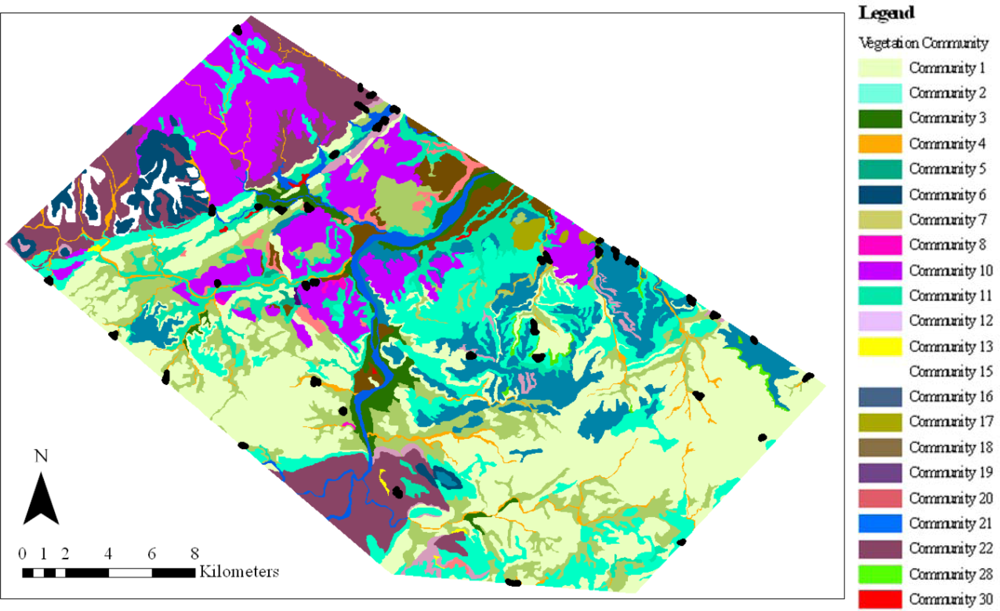
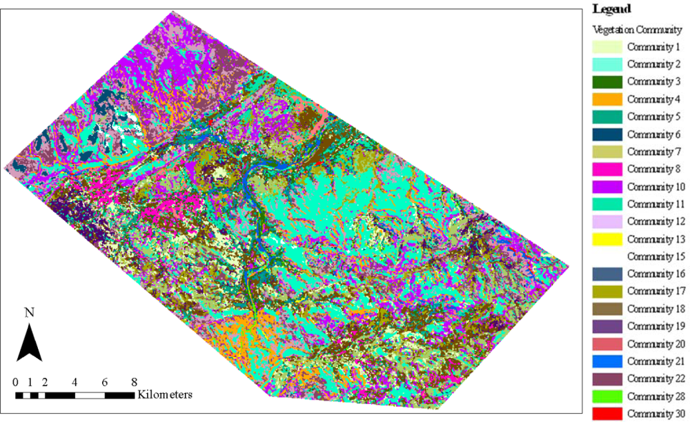
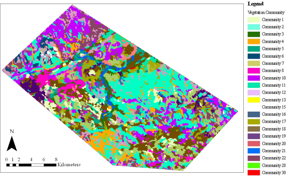
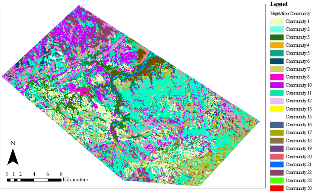
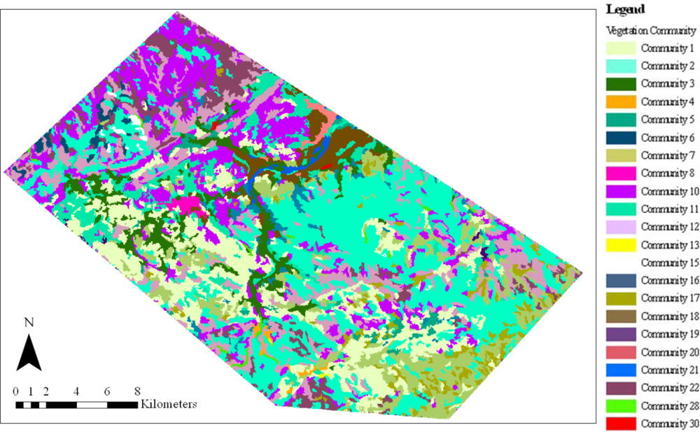
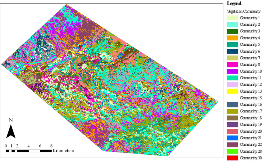
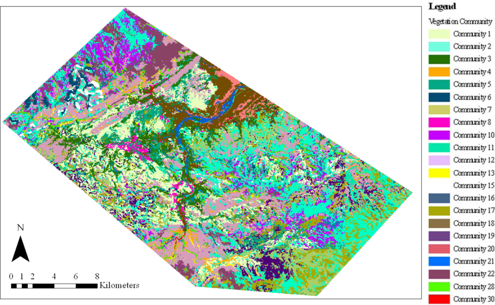
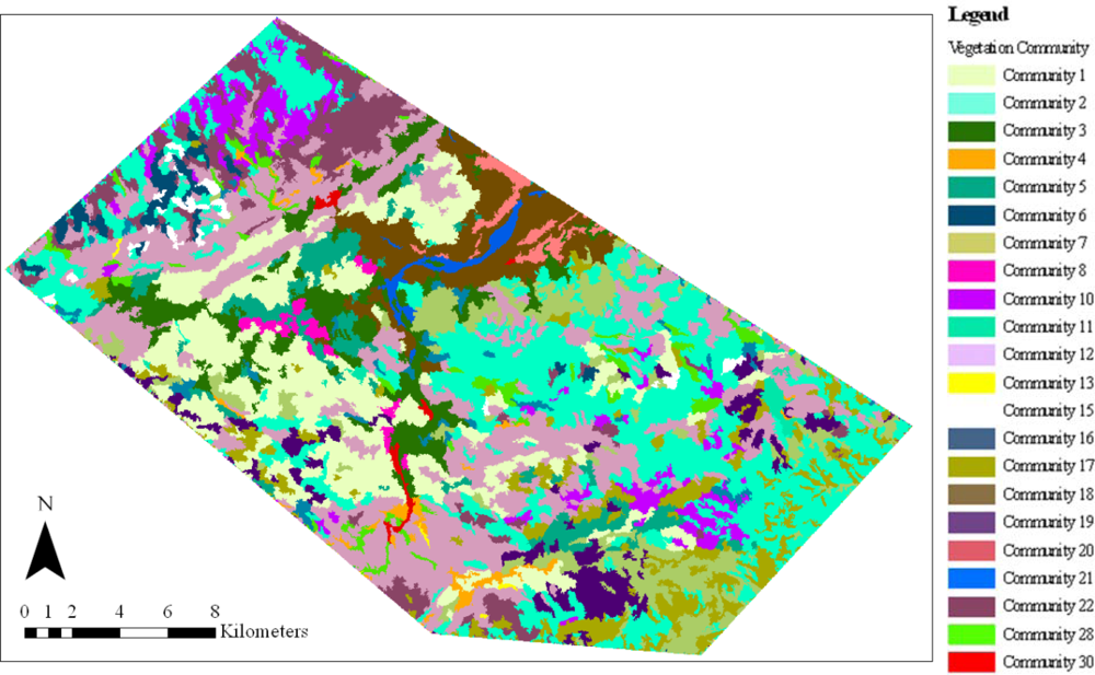
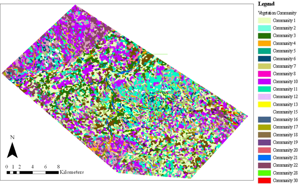
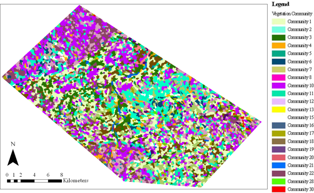
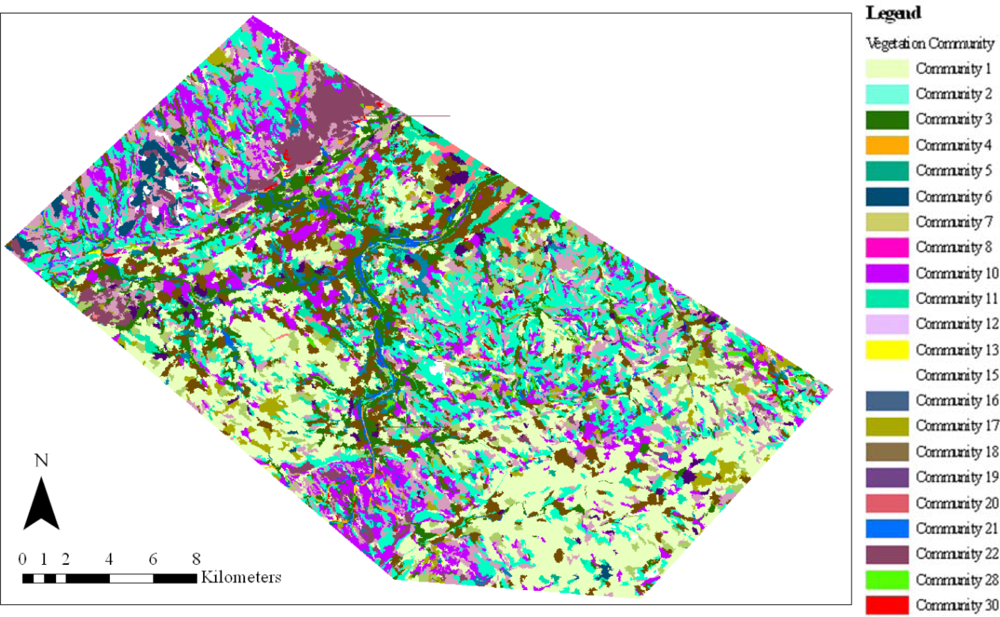
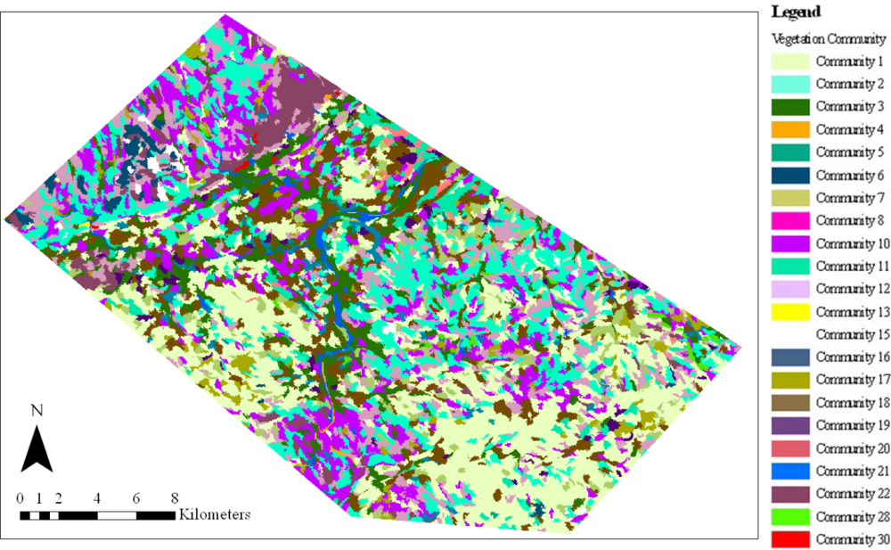
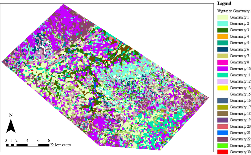
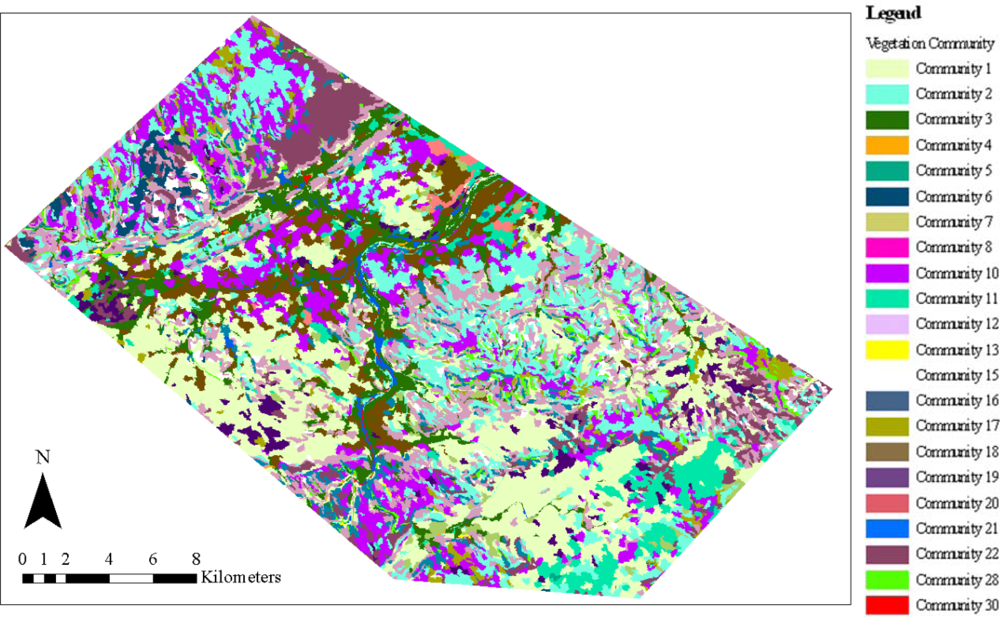
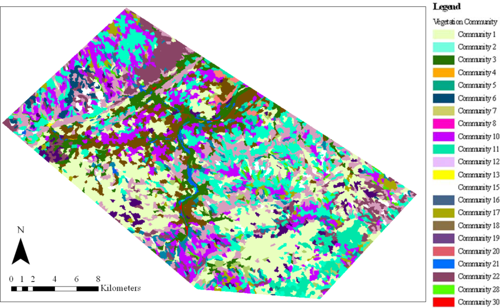
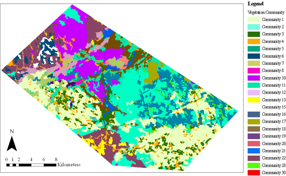
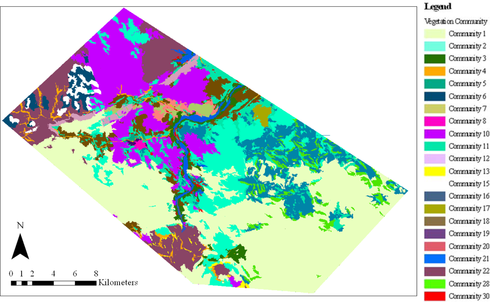
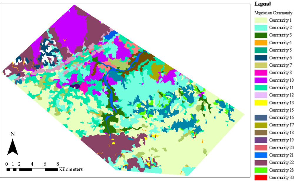
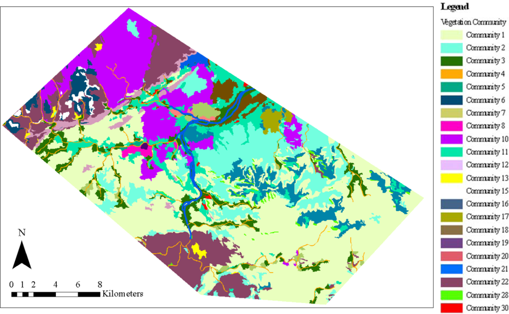
Appendix 2. Output vegetation community maps for the seven mapping approaches, three image dataset and at the 1:25,000 and 1:100,000 spatial scales. API: 1:50,000 aerial photography mosaic at 1:25,000 and 1:100,000. Datum: GDA94, Coordinate System: Decimal Degrees 129.578–15.877, 129.825–15.597, 129.469–15.534, 129.688–15.7.


| Component | Subcomponent | Detailed Costs and Time Invested |
|---|---|---|
| (1) Field data acquisition and preparation* | Field sampling* Plant identification and databasing* Multi-variate analysis and vegetation classification* | Working hours, staff salaries, staff travel allowance, helicopter hire cost (wet rate), vehicle lease cost, fuel cost Working hours, staff salaries |
| (2) Image data acquisition and preparation | Image acquisition Image pre-processing | Working hours, staff salaries, image cost Working hours, staff salaries |
| (3) Image Classification | API linework API attribution PBIA training PBIA classification GEOBIA segmentation GEOBIA training GEOBIA classification | Working hours, staff salaries |
| (4) Accuracy Assessment* | Accuracy assessment* | Working hours, staff, salaries |
| Component | Subcomponent | Detailed Cost (AU$) | Total Cost (AU$) |
|---|---|---|---|
| Field data acquisition and preparation | Field sampling | Salaries*: 59,227 Travel allowance: 15,746 Vehicle costs: 5,120 Helicopter hire: 28,700 | 120,000 |
| Plant identification and data basing | Plant identification*: 196,700 Data basing*: 5,000 | 201,700 | |
| Multi-variate analysis and vegetation classification | Multi-variate analysis*: 2,260 Vegetation classification*: 750 | 3,010 | |
| Accuracy assessment | Generating training areas from field data*: 1,400 | 1,890 | |
| Accuracy assessment*: 490 | |||
| TOTAL | 326,600 |
Share and Cite
Lewis, D.; Phinn, S.; Arroyo, L. Cost-Effectiveness of Seven Approaches to Map Vegetation Communities — A Case Study from Northern Australia’s Tropical Savannas. Remote Sens. 2013, 5, 377-414. https://doi.org/10.3390/rs5010377
Lewis D, Phinn S, Arroyo L. Cost-Effectiveness of Seven Approaches to Map Vegetation Communities — A Case Study from Northern Australia’s Tropical Savannas. Remote Sensing. 2013; 5(1):377-414. https://doi.org/10.3390/rs5010377
Chicago/Turabian StyleLewis, Donna, Stuart Phinn, and Lara Arroyo. 2013. "Cost-Effectiveness of Seven Approaches to Map Vegetation Communities — A Case Study from Northern Australia’s Tropical Savannas" Remote Sensing 5, no. 1: 377-414. https://doi.org/10.3390/rs5010377
APA StyleLewis, D., Phinn, S., & Arroyo, L. (2013). Cost-Effectiveness of Seven Approaches to Map Vegetation Communities — A Case Study from Northern Australia’s Tropical Savannas. Remote Sensing, 5(1), 377-414. https://doi.org/10.3390/rs5010377