Article

Evaluation of Clear-Sky Incoming Radiation Estimating Equations Typically Used in Remote Sensing Evapotranspiration Algorithms

1
National Institute for Environmental Studies, 16-2 Onogawa, Tsukuba, Ibaraki 305-8506, Japan
2
Civil & Environmental Engineering, University of Connecticut, 261 Glenbrook Road, Storrs, CT 06269, USA
3
Illinois State Water Survey, UIUC, 2204 Griffith, Champaign, IL 61820, USA
4
Department of Plant and Environmental Sciences, New Mexico State University, Las Cruces, NM 88003, USA
5
Ecosystem Processes and Dynamics, CSIR, PO Box 395, Pretoria 0001, South Africa
*
Author to whom correspondence should be addressed.
Remote Sens. 2013, 5(10), 4735-4752; https://doi.org/10.3390/rs5104735
Submission received: 23 July 2013 / Revised: 17 September 2013 / Accepted: 18 September 2013 / Published: 25 September 2013

Abstract

:
Net radiation is a key component of the energy balance, whose estimation accuracy has an impact on energy flux estimates from satellite data. In typical remote sensing evapotranspiration (ET) algorithms, the outgoing shortwave and longwave components of net radiation are obtained from remote sensing data, while the incoming shortwave ( R S ) and longwave ( R L ) components are typically estimated from weather data using empirical equations. This study evaluates the accuracy of empirical equations commonly used in remote sensing ET algorithms for estimating R S and R L radiation. Evaluation is carried out through comparison of estimates and observations at five sites that represent different climatic regions from humid to arid. Results reveal (1) both R S and R L estimates from all evaluated equations well correlate with observations (R2 ≥ 0.92), (2) R S estimating equations tend to overestimate, especially at higher values, (3) R L estimating equations tend to give more biased values in arid and semi-arid regions, (4) a model that parameterizes the diffuse component of radiation using two clearness indices and a simple model that assumes a linear increase of atmospheric transmissivity with elevation give better R S estimates, and (5) mean relative absolute errors in the net radiation (Rn) estimates caused by the use of R S and R L estimating equations varies from 10% to 22%. This study suggests that Rn estimates using recommended incoming radiation estimating equations could improve ET estimates.

1. Introduction

Net radiation (Rn) is a key component of the energy balance, whose estimation accuracy has an impact on energy flux estimates from remotely sensed data. In typical algorithms that handle remote sensing data, evapotranspiration (ET) is estimated as a residual of Rn after accounting for sensible heat flux (H) and soil heat flux (G) [14]; G is estimated from empirical equations that relate G/Rn to vegetation index, and H is estimated such that the maximum value of H over a “hot” surface does not exceed Rn. Llasat and Snyder reported that 65%–85% of the error in Rn estimation directly propagates to crop-reference ET in the Catalonia region of Spain [5]. Sun et al. showed that a 10% error in Rn could result in a 25% error in actual ET when the latter is estimated through the Sim-ReSET algorithm over an irrigated crop field in a semi-arid climate [6].
In algorithms that estimate energy fluxes from remotely senses data, Rn is estimated by summing up estimates of its shortwave and longwave components:
R n = R S R S + R L R L = ( 1 α ) R S + R L ε s σ T s 4
where R S is the incoming shortwave radiation, R S is the outgoing shortwave radiation, R L is the incoming longwave radiation, R L is the outgoing longwave radiation, α is the surface albedo, εs is the surface emissivity, σ is the Stefan-Boltzmann constant (i.e., 5.670373×10⁻⁸ W/m2/K4), and Ts [K] is the surface temperature. The incoming components ( R S and R L ) might be indirectly estimated from remote sensing data and atmospheric profile observational data through radiative transfer models [710], but they are typically estimated from available weather station data using empirical but straightforward equations in remote sensing ET algorithms [1,6,1113]. The outgoing components ( R S and R L ) could be directly estimated from remote sensing optical and thermal information of land surface.
Several studies have been conducted to evaluate empirical estimating equations of incoming components. For example, Gubler et al. evaluated clear-sky R S and all-sky R L parameterizations in Switzerland [14]; Trnka et al. evaluated various empirical formulae of R S in Central European lowlands [15]; Marthews et al. evaluated contrasting semi-empirical estimation schemes of R L under clear and cloudy conditions over a tropical lowland forest site [16]; Carmona et al. estimated daytime R L under clear and cloudy skies conditions over a sub-humid region [17]. However most of those studies were limited to either one or few locations, and Rn calculated from R S and R L was not evaluated.
The purpose of this study was to evaluate the accuracy of commonly used empirical equations that estimate R S , R L , and then Rn from weather station data under clear sky conditions. Our approach was to compare these estimates to ground-based measurements (observations) across continents with contrasting climates and land cover types. We considered 7 equations for estimating R S and 6 equations for estimating R L . The study was limited to clear-sky conditions (given our focus on satellite remote sensing ET algorithms and the fact that satellite remote sensing cannot provide useful visual and thermal data of land surface during cloudy sky conditions).
This paper is organized as follows. Section 2 provides the commonly-used estimating equations for R S and R L under clear sky conditions. Section 3 presents an overview of the ground reference sites and measurements and the evaluation metrics employed. The results of the comparison of R S , R L , and Rn estimates against observations are provided and discussed in Section 4. Conclusions are drawn in Section 5.

2. Methodology

2.1. Estimating Equations for Incoming Shortwave Radiative Flux ( R S )

2.1.1. Theoretical Framework

R S is determined by the solar constant (S0, 1,367 W/m2), solar zenith angle (θ, rad), atmospheric transmissivity (τ), and Earth-Sun distance in astronomical unit (d, AU):
R S = τ S 0 d 2 cos θ
The Earth-Sun distance can be calculated using the day of year (DOY) [11]:
d = 1 + 0.0167 sin ( 2 π DOY 93.5 365 )
d varies between 0.9833 AU (3–5 January) and 1.0167 AU (3–7 July).
The solar zenith angle can be calculated using geographical latitude (φ, rad), solar declination (δ, rad), solar hour angle (ω, rad), and topographic data [18,19]:
  • For sloping surfaces,
    cos θ = sin δ ( sin ϕ cos s cos ϕ sin s cos γ ) + cos δ cos ω ( cos ϕ cos s + sin ϕ sin s cos γ ) + cos δ sin γ sin s sin ω
  • For horizontal surfaces,
    cos θ = sin δ sin φ + cos δ cos φ cos ω
where s [rad] and γ [rad] are the slope and the azimuth calculated from digital elevation models.
The solar hour angle is calculated using local time (t, h):
ω = π t 12 12
The solar declination is calculated using DOY:
δ = 0.4093 sin ( 2 π DOY + 284 365 )
The challenge in R S estimation lies in obtaining accurate estimates of atmospheric transmissivity τ. A number of empirical equations have been proposed for estimating τ.

2.1.2. Equations for Estimating Clear-Sky R S

We considered the following estimating equations commonly used in remote sensing ET algorithms for estimating R S using weather station data:
  • SW1—the equation of Tasumi et al. [20],
  • SW2—the equation of Zillman [21],
  • SW3—the modified equation of Zillman [21],
  • SW4—the equation of Shine [22],
  • SW5—the modified equation of Shine [22],
  • SW6—the scheme of Allen et al. [23], and
  • SW7—the scheme of Kondo [24].
SW1—The equation of Tasumi et al. assumes that the atmospheric transmissivity in cloudless sky conditions is a constant value of 0.75 just above sea surface, and increases linearly with elevation [20]. The equation is given as:
R S = τ S 0 d 2 cos θ = ( 0.75 + 2 × 10 5 E ) S 0 d 2 cos θ
where E [m] is the elevation above mean sea level. This equation was, for example, used for estimation of daily actual ET in North China [13].
SW2—The equation of Zillman uses solar zenith angle and water vapor pressure (e0) at the screen level [21]:
R S = S 0 cos 2 θ 1.085 cos θ + e 0 ( 2.7 + cos θ ) × 10 2 + 0.1 = cos θ 1.085 cos θ + e 0 ( 2.7 + cos θ ) × 10 2 + 0.1 S 0 cos θ
where e0 is in kPa. The seasonal variation of the Earth-Sun distance is not considered in this equation. This equation was adopted to estimate net radiation from Moderate Resolution Imaging Spectroradiometer (MODIS) data [25], and also was used in existing remote sensing ET algorithms [6,26,27].
SW3—The modified equation of Zillman [21]. We modified SW2 by varying the Earth-Sun distance seasonally:
R S = cos θ 1.085 cos θ + e 0 ( 2.7 + cos θ ) × 10 2 + 0.1 S 0 d 2 cos θ
SW4—The equation of Shine is a modified version of SW2 by adjusting the coefficients to well agree with the detailed calculations of a method as a function of cloud thickness and surface albedo [22]:
R S = S 0 cos 2 θ 1.2 cos θ + e 0 ( 1.0 + cos θ ) × 10 2 + 0.0455 = cos θ 1.2 cos θ + e 0 ( 1.0 + cos θ ) × 10 2 + 0.0455 S 0 cos θ
This equation also ignores the seasonal variation of the Earth-Sun distance.
SW5—The modified equation of Shine [22]. We modified SW4 by varying the Earth-Sun distance seasonally:
R S = cos θ 1.2 cos θ + e 0 ( 1.0 + cos θ ) × 10 2 + 0.0455 S 0 d 2 cos θ
SW6—The equation of Allen et al. [23]:
R S = τ S 0 d 2 cos θ = ( K Bo + K Do ) S 0 d 2 cos θ
where KBo is the clearness index for direct beam radiation and KDo is the clearness index for diffuse beam radiation.
The KBo is calculated as:
K Bo = 0.98 e 0.00146 P K t sin β 0.075 ( W sin β ) 0.4
where Kt is the empirical turbidity coefficient, P [kPa] is the surface atmospheric pressure, β [rad] is the angle of the sun above the horizon, and W [mm] is the equivalent depth of precipitable water in the atmosphere. Kt varies between 0 (extremely turbid, dusty or polluted air) and 1 (clean air, typical of agricultural and natural vegetation regions). β is calculated from solar declination (δ) geographical latitude (φ), and solar hour angle (ω) as sinβ = sinδ sinφ +cosδ cosφ cosω. W is calculated from the water vapor pressure at the screen level (e0) and atmospheric pressure (P) as W = 0.14e0 P+2.1.
The KDo is calculated from KBo as:
K Do = { 0.35 0.36 K Bo , K Bo 0.15 0.18 + 0.82 K Bo , 0.065 < K Bo < 0.15 0.10 + 2.08 K Bo , K Bo 0.065
SW7—The equation of Kondo considers the effect of atmospheric optical length, aerosol, vapor, and land surface albedo on shortwave radiation [24]:
R S = τ S 0 d 2 cos θ = ( C + 0.70 e MF ln 10 ) ( 1 I ) ( 1 + J ) S 0 d 2 cos θ
where,
M = ( P / P 0 ) / cos θ
C = 0.21 0.2 η
F = 0.056 + 0.16 η 2
J = ( 0.066 + 0.34 η 2 ) ( α 0.15 )
I = 0.014 ( M + 7.0 + 2.0 F w ) F w
F w = 0.4343 ln ( W / 10 )
W = 1.234 W e 0.21
W e = { e 0.0622 t d + 1.985 b , t d < 5 e 0.0714 t d + 2.003 b , 5 < t d < 23 e 0.0345 t d + 2.851 b , 23 < t d
b = { 0 , 99 < P < P 0 2.3026 ( 1 P / P 0 ) 2 , P > P 0 or P < 99
where M is the optical length of atmosphere, P0 [kPa] is the standard atmospheric pressure at sea level, C and F are two aerosol optical parameters related to the turbidity coefficient (η, 0.03 for clear sky conditions), J is the parameter that accounts for the effect of surface albedo (as a constant of 0.2) on scattered light, I is the vapor optical parameter, Fw is an intermediate variable used to calculate I, W [mm] is the atmospheric precipitable water, We is an intermediate variable for W estimation, td [°C] is the dew point temperature, and b is the parameter that accounts for the effect of air pressure on atmospheric precipitable water. The SW7 scheme was used in the remote sensing ET algorithm of Nishida et al. [12], among others.

2.1.3. Summary of Clear-Sky R S Estimating Equations

Shortwave radiation is the sum of a direct beam component and a diffuse component. Both components depend on atmospheric transmissivity (i.e., integrated effect of molecular and particulate absorption and scattering). Although these processes possess a spectral variability, simple models that compute integrated atmospheric transmissivity are often used in various remote sensing algorithms. Methods SW1 to SW5 are very crude approximations of the integrated shortwave radiation. The diffuse component is parameterized in SW6 using two clearness indices KBo and KDo, with the clearness index for the diffuse component that depends on the clearness index for the direct component and the latter is computed from an empirical turbidity coefficient which is assigned a constant value (equal to 1.0) for clear sky conditions. SW7 is more complex, and it is based on a number of relations that rely on two aerosol optical parameters related to the turbidity coefficient which is assigned a constant value for clear sky conditions. Molecular absorption is parameterized either from elevation (SW1) or from water vapor pressure (SW2 to SW5) or from atmospheric precipitable water (SW6 and SW7). The only difference between SW2 and SW3, and between SW4 and SW5, is the accounting for (or lack thereof) seasonal variation of the Earth-Sun distance.

2.2. Estimating Equations for Incoming Longwave Radiative Flux ( R L )

2.2.1. Theoretical Framework

R L can be calculated as:
R L = ε a σ T a 4
where εa is the atmospheric emissivity, and Ta [K] is the screen-level air temperature. Ta can be obtained from weather station data, but εa depends on vertical profiles of temperature and radiatively active constituents that are not available from typical weather station data. εa is often estimated from weather station data using empirical equations, and therefore the challenge in R L estimation lies in obtaining accurate estimates of εa

2.2.2. Equations for Estimating Clear Sky R L

We considered the following estimating equations commonly used in remote sensing ET algorithms for estimating R L using weather station data:
  • LW1—the equation of Brutsaert [28],
  • LW2 (a–d)—the equation of Prata [29] and its modified equations, and
  • LW3—the scheme of Kondo [24].
LW1—The equation of Brutsaert uses air temperature and vapor pressure to estimate R L [28]:
R L = ε a σ T a 4 = 1.24 ( 10 e 0 T a ) 1 / 7 σ T a 4
where air temperature [K] and vapor pressure [kPa] measurements are taken at the screen level. This equation was used by Gao et al. [13], among others.
LW2(a–d)—The equation of Prata uses atmospheric precipitable water and air temperature to estimate R L [29]:
R L = ε a σ T a 4 = [ 1 ( 1 + W ) e ( 1.2 + 3.0 W ) 0.5 ] σ T a 4
where W [cm] is the atmospheric precipitable water. W is typically estimated from empirical equations involving air temperature and/or vapor pressure. This equation has been adopted for estimation of net radiation from MODIS data [25]. We considered four different empirical equations for estimating W:
Prata [ 29 ] : W = 465 ( e 0 / T a )
Kondo [ 24 ] : W = 0.1234 W e 0.021
Reitan [ 30 ] : ln W = 0.1102 + 0.06141 t d
Ven a ¨ l a ¨ inen [ 31 ] : W = 0.71104 ( 493 e 0 / T a ) 0.032003
Depending on the W equation, different LW equations can be distinguished:
LW3—The equation of Kondo uses We and air temperature to estimate clear-sky R L [24]:
R L = ( 0.59 + 0.038 ln W e + 0.011 ln 2 W e ) σ T a 4 ) .
This equation was used by Nishida et al. [12], among others.

2.2.3. Summary of Clear-Sky R L Estimating Equations

R L can be calculated directly from air temperature and profile of atmospheric emissivity. While air temperature data are available from weather stations, atmospheric emissivity profiles are not. Simple models that compute integrated emissivity based on weather station data are often used in various remote sensing algorithms. Integrated atmospheric emissivity can be estimated from vapor pressure and air temperature at the screen level (LW1, LW2a, LW2d) or from dew point temperature (LW2b, LW2c, LW3). The equations also differ in their functional forms and parameter values.

3. Data and Approach

3.1. Data

Our data came from flux tower stations at five sites (three sites in China, one site in South Africa, and one site in USA). Table 1 provides salient features of the sites, observed variables and data period. The sites represent a wide range of climatic conditions (humid to arid), elevations (28 m a.s.l. (meter above sea level) to 1177 m a.s.l.) and land cover conditions (paddy, irrigated crop, shrub, savanna, and pecan orchard). The sites in China have 30-min measurements of Ta, relative humidity (RH), P, Ts, R S , R S , R L , R L , and Rn [32]. The site in South Africa has 30-min measurements of Ta, RH, P, R S , and R S [33], and the site in USA has 60-min measurements of Ta, RH, P, R S , and Rn [34].
The instruments were well maintained and calibrated yearly, and so the measurement errors can be safely assumed to arise only from the known instrument manufacturing errors. For example, a Q7 net radiometer (see http://www.campbellsci.com/q7-1-l for details) installed at the OPEC site has an accuracy of ±2.5%, while CNR1 net radiometers (see http://www.campbellsci.com/cnr1-l for details) installed at the other four sites have an accuracy of ±10% for daily totals. More information on the instruments and data quality is available in [3234].

3.2. Approach

Our approach was to evaluate estimates of R S , R L , and Rn through comparison of the estimates with flux tower observations. The estimates were obtained from empirical equations using input data (e.g., air temperature) provided by the flux tower observations. We used the following statistics to measure the performance of the estimates:
ME = 1 n i = 1 n ( E i O i )
MAE = 1 n i = 1 n | E i O i |
MRE = 1 n i = 1 n | E i O i | O i
where Ei is the estimated value, Oi is the flux tower observed value, ME is the mean error, MAE is the mean absolute error, MRE is the mean relative absolute error, and n is the number of pairs of estimated and observed values.

4. Results and Discussions

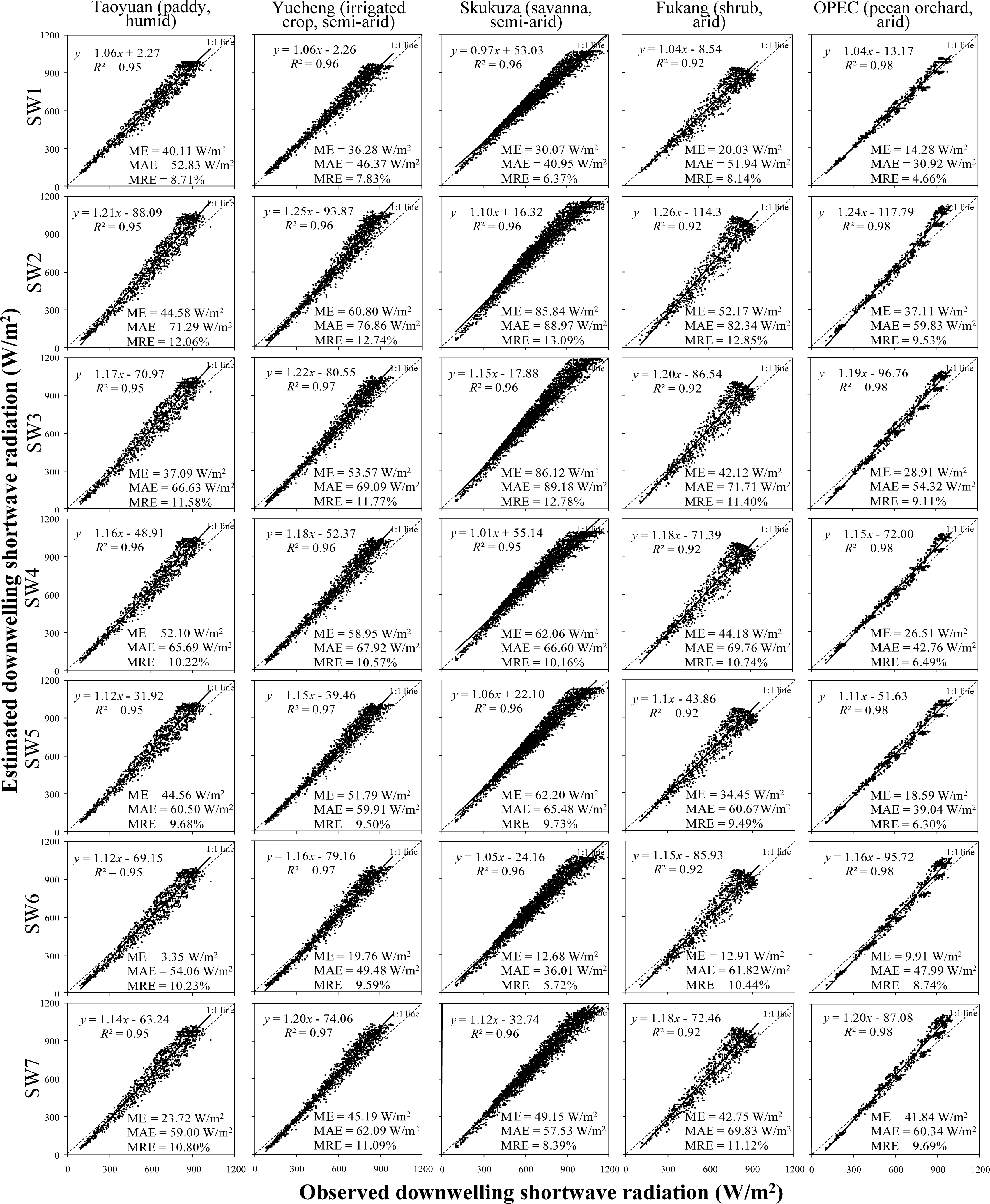
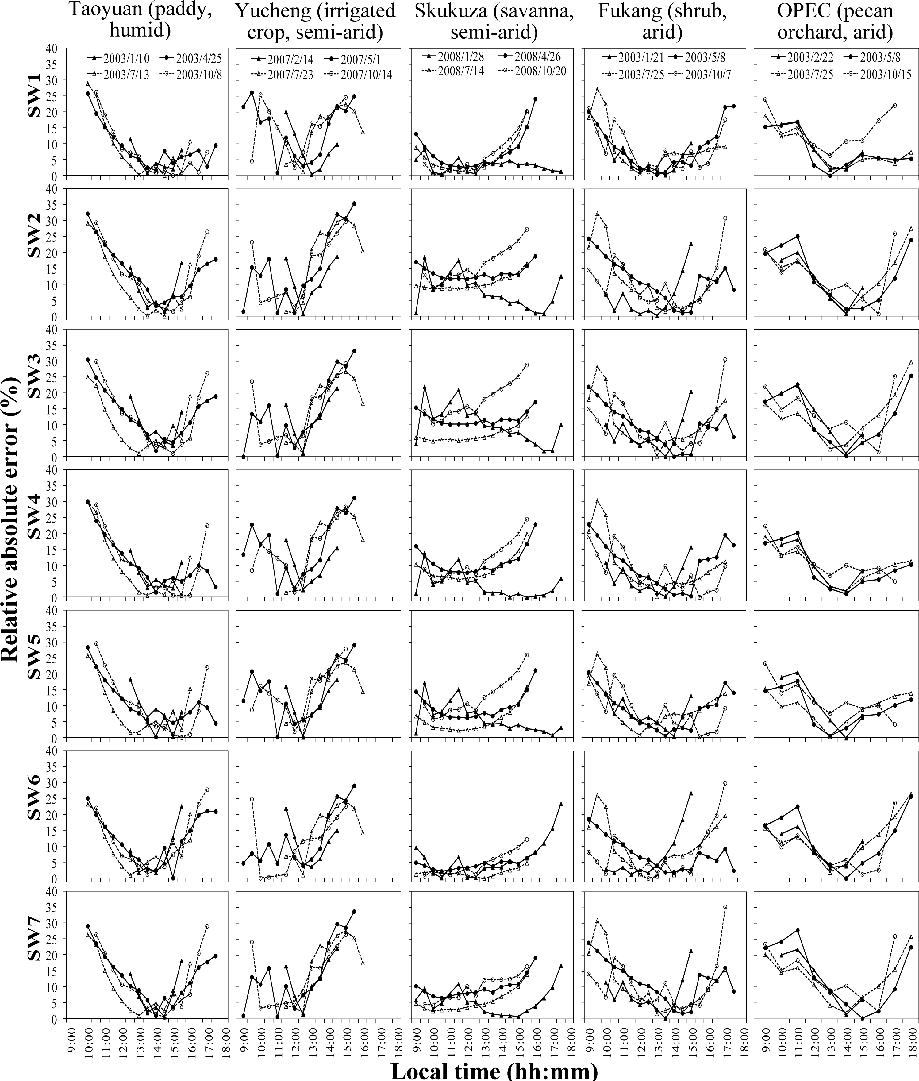
4.1. Evaluation of Clear-Sky Incoming Shortwave Radiation ( R S ) Estimating Equations

Only clear-sky cases were collected. The total number of clear-sky cases was 999, 1,449, 2,948, 897 and 738 cases, at the Taoyuan, Yucheng, Skukuza, Fukang, and OPEC sites, respectively. Figure 1 presents comparison of R S estimates and observations. We note that scattered points in Figure 1 represent 60-min average for the OPEC site (last column), and 30-min average for the other sites. There is a high correlation (R2 ≥ 0.92) between the estimates and observations. The bias (i.e., ME) varies from 3.35 W/m2 to 86.12 W/m2, the variability (i.e., MAE) varies from 30.92 W/m2 to 89.18 W/m2, and the relative variability (i.e., MRE) varies from 4.66% to 13.09%. According to ME, SW6 performs better than the other methods at all sites (ME: 3.35–19.76 W/m2). According to MRE, SW1 performs better than the other methods at four of the five sites (MRE: 4.66%–8.71%). Mainly because of location-specific empirical coefficients, the simple equations (SW2–SW5) that estimate transmissivity based on vapor pressure and the complex SW7 that involves several equations give worse performance (ME: 18.59–86.12 W/m2; MRE: 6.30%–13.09%). The R S values from SW1 to SW7 tend to be overestimated over the higher ranges, which indicates that atmospheric transmissivity tends be overestimated when R S values are relatively high. The SW1 and SW6 perform better because both estimate atmospheric transmissivity better.
Figure 2 shows the relative absolute errors (for four typical days in four seasons at five sites) for each SW model in the daytime from 9:00 to 18:00 during which the diurnal variation of solar radiation can be obtained in the four seasons at the five sites. One observes that the relative absolute errors are higher in the morning and late afternoon. This may be due to the significance diffuse shortwave component in the morning and late afternoon.

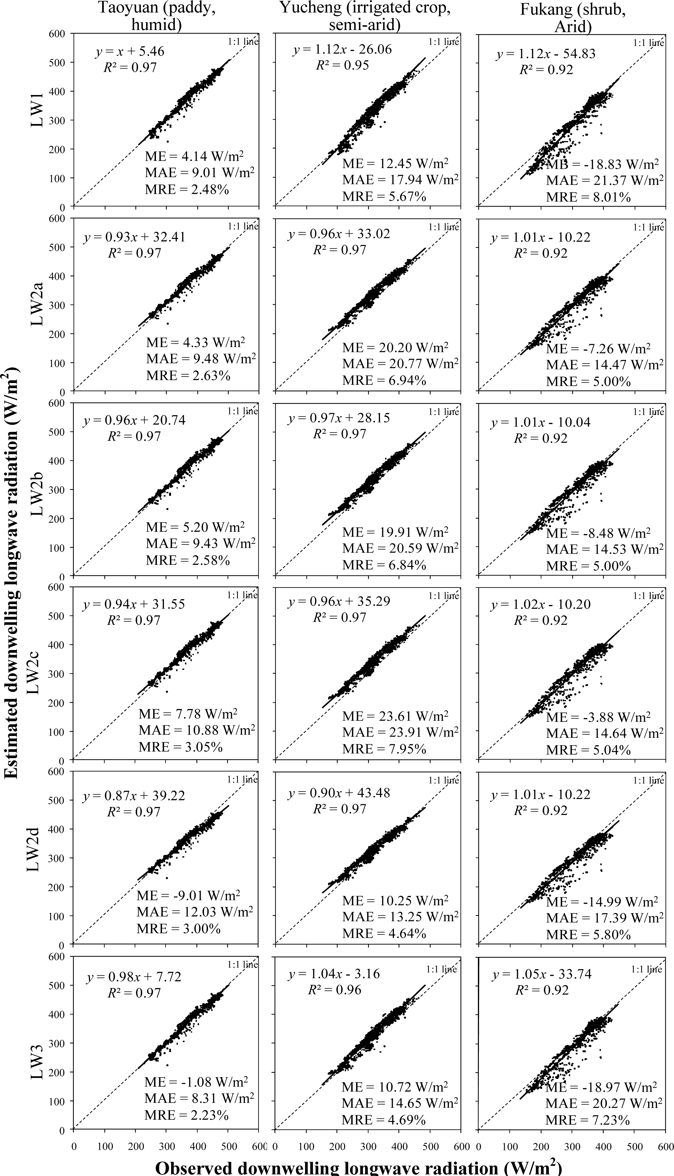
4.2. Evaluation of Clear-sky Incoming Longwave Radiation ( R L ) Estimating Equations

Figure 3 presents comparison of R L estimates and observations. There is a high correlation (R2 ≥ 0.92) between the estimates and observations. The relative variability (i.e., MRE) varies from 2% to 8%, which is better than that of R S estimates. All equations give negatively-biased estimates (ME from −8.97 W/m2 to −3.88 W/m2) at the Fukang site (arid), positively-biased estimates (ME from 10.25 W/m2 to 23.61 W/m2) at the Yucheng site (semi-arid), and relatively less-biased estimates (ME from −9.01 W/m2 to 7.78 W/m2) at the Taoyuan site (humid). This suggests that all the equations considered were not calibrated well for semi-arid and arid regions. The equation that gives the best R L estimate depends on the climate/site: LW3 at the humid site, LW2d and LW3 at the semi-arid site, and LW2c at the arid site. This indicates that the empirical R L estimating equations perform better while local climatic conditions are similar to that under which they were developed.
Figure 4 shows the relative absolute errors (for four typical days in four seasons at three sites) for each LW model. In most cases, there is no pronounced diurnal variation in the estimates.

4.3. Evaluation of Clear-Sky Net Radiation (Rn) Estimating Equations

As discussed in Section 1, Rn is typically estimated as the sum of the incoming and outgoing shortwave and longwave radiation fluxes. Here, we assess the impacts of R S and R L estimating equations on the accuracy of Rn estimates. We compared the Rn estimates (obtained using R S and R L estimates and R S and R L observations) to Rn observations at the three sites in China. Table 2 presents comparison results for all combinations of estimating equations. The MRE varies from 10.53% to 21.57%, depending on the site and estimating equation. The MRE is smaller at the humid site (11.14% to 15.29%) and semi-arid site (10.53% to 16.73%) compared to the arid site (13.65% to 21.57%). The R S and R L estimating equations that give the best Rn estimate are: SW1 and LW2d in the humid site, SW1 and LW2d in the semi-arid site, and SW1 and LW3 in the arid site. This is consistent with our earlier finding that SW1 performs better for estimating R S (see Figure 1). However, the best estimating equations for R L (LW3 at the humid and semi-arid sites, and LW2c at the arid site; See Figure 3) are not involved in the set of equations that give the best Rn estimate. This is because the R L estimates that have large negative biases (therefore not the best R L estimates) tend to counter the large positive biases in the SW1 R S estimates, leading to the best Rn estimates.

4.4. Suggestions on Incoming Radiation Estimation Equations for Remote Sensing ET Algorithms and Further Studies

This study reveals that the R S estimating equations with less location-specific empirical coefficients tend to perform better for the wide ranges of climates and land cover types. This suggests that R S estimating equations with empirical coefficients should be well calibrated before they are used out of the regions where they were developed. Therefore, the developers and users of remote sensing ET algorithms should select incoming radiation estimation equations with less empirical coefficients or well-calibrated equations for estimating Rn and then ET. We conducted a case study at an arid site (Fukang) to demonstrate the improvement of remote sensing-based ET estimates using recommended incoming radiation estimating equations. The SW2 and LW2a equations originally embedded in the Sim-ReSET model were replaced by the SW6 and LW2c equations recommended in this study, respectively. By comparing with eddy covariance flux measurements, the Sim-ReSET model using the SW6 and LW2c equations could better estimate actual ET than that using the original SW2 and LW2a equations, with the MRE decreasing from 30% to 21% (see Figure 5). Refer to Sun et al. [6,35] for details about the Sim-ReSET model and ground measurements.
Although our evaluations on incoming radiation estimation equations span wide ranges of climate and land cover types, it is still hard to affirm that the best estimating equations in this study work best across the lands. For universal empirical estimating equations for R S , R L and then Rn, robust radiative transfer models could be used to simulate full ranges of climates and land cover types to obtain universal empirical coefficients or make a look-up table of empirical coefficients in further studies. Meanwhile, more ground observations representing all kinds of climates land cover types are in the request to validate the results of simulations.

5. Conclusions

We have evaluated the accuracy of seven estimating equations for incoming shortwave radiative flux ( R S ) and six estimating equations for incoming longwave radiative flux ( R L ) by comparing the estimates to flux tower observations at five sites that represent humid; semi-arid and arid climates. Our conclusions can be summarized as:
  • Both R S and R L estimates from all evaluated equations well correlate with observations (R2 ≥ 0.92).
  • The R S estimating equations tend to overestimate, especially at higher values. The equations give large errors in the morning and late afternoon hours, where diffuse radiation is substantial. Of all the estimating equations, the equation treats the diffusive radiation component using two clearness indices and the equation assumes a linear increase of atmospheric transmissivity with elevation give the best estimates, and the mean relative absolute errors (MRE) are less than 10%. The equations that estimate atmospheric transmissivity from vapor pressure data or involve several complex relations produce worse results, and their MREs tend to be more than 10%.
  • The R L estimating equations produce biased estimates at the arid and semi-arid sites (MRE: >4%) and less-biased estimates at the humid site (MRE: <3%).
  • As a whole, the R L estimating equations tend to perform better than the R S estimating equations.
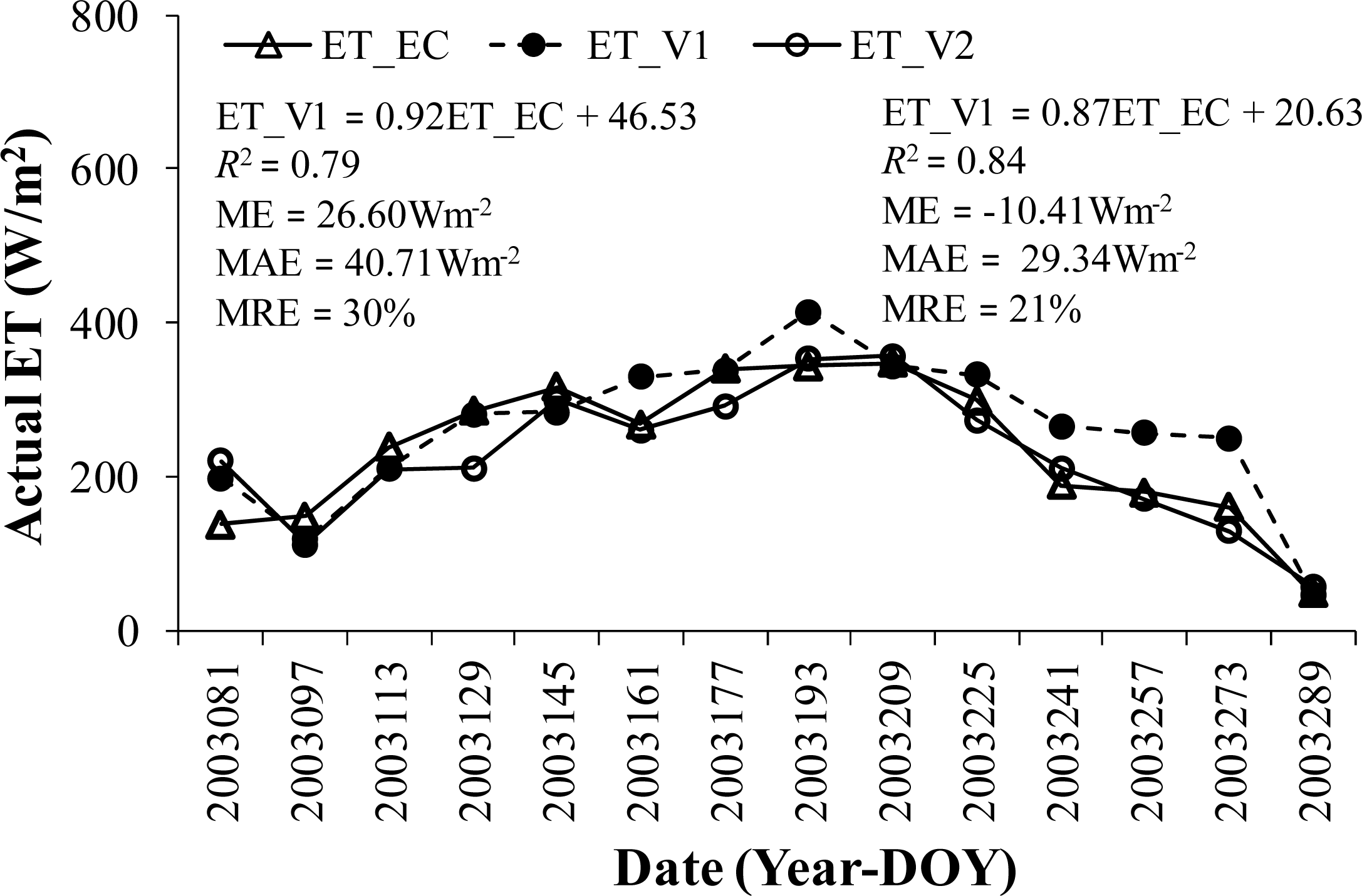
  • The MRE in the net radiation (Rn) estimates caused by the use R S and R L estimating equations varies from 10% to 22%. The equation that gives the best estimate of Rn involves (1) the best R S estimating equation for R S estimation, and (2) the R L estimating equation that gives the largest negative bias or the smallest positive bias for R L estimation to compensate for the large positive bias in the R S estimates.
This study suggests that incoming radiation estimation equations with less empirical coefficients or well-calibrated equations could be used for better estimating Rn and then evapotranspiration (ET) in remote sensing ET algorithms. The best Rn estimates still have at least 10% error, which will be inevitably propagated to ET estimates. Therefore, the accuracy of Rn estimation should be carefully considered in developing and applying remote sensing ET algorithms in future studies and applications.

Acknowledgments

This study was supported by the NASA NIP Grant NNX08AR31G to the University of Connecticut and by the Environment Research and Technology Development Fund (E-1203) of the Ministry of the Environment, Japan. Authors thank anonymous reviewers and editors for their constructive comments.

Conflicts of Interest

The authors declare no conflict of interest.

References

  1. Ruhoff, A.L.; Paz, A.R.; Collischonn, W.; Aragao, L.E.O.C.; Rocha, H.R.; Malhi, Y.S. A MODIS-based energy balance to estimate evapotranspiration for clear-sky days in Brazilian tropical savannas. Remote Sens 2012, 4, 703–725. [Google Scholar]
  2. Mariotto, I.; Gutschick, V.P. Non-lambertian corrected albedo and vegetation index for estimating land evapotranspiration in a heterogeneous semi-arid landscape. Remote Sens 2010, 2, 926–938. [Google Scholar]
  3. Cuenca, R.; Ciotti, S.; Hagimoto, Y. Application of Landsat to evaluate effects of irrigation forbearance. Remote Sens 2013, 5, 3776–3802. [Google Scholar]
  4. Hankerson, B.; Kjaersgaard, J.; Hay, C. Estimation of evapotranspiration from fields with and without cover crops using remote sensing and in situ methods. Remote Sens 2012, 4, 3796–3812. [Google Scholar]
  5. Llasat, M.C.; Snyder, R.L. Data error effects on net radiation and evapotranspiration estimation. Agric. For. Meteorol 1998, 91, 209–221. [Google Scholar]
  6. Sun, Z.G.; Wang, Q.X.; Matsushita, B.; Fukushima, T.; Ouyang, Z.; Watanabe, M. Development of a simple remote sensing evapotranspiration model (Sim-ReSET): Algorithm and model test. J. Hydrol 2009, 376, 476–485. [Google Scholar]
  7. Gueymard, C.A. Clear-sky irradiance predictions for solar resource mapping and large-scale applications: Improved validation methodology and detailed performance analysis of 18 broadband radiative models. Solar Energy 2012, 86, 2145–2169. [Google Scholar]
  8. Liang, S.L.; Wang, K.C.; Zhang, X.T.; Wild, M. Review on estimation of land surface radiation and energy budgets from ground measurement, remote sensing and model simulations. IEEE J. Sel. Top. Appl. Earth Obs. Remote Sens 2010, 3, 225–240. [Google Scholar]
  9. Wu, H.R.; Zhang, X.T.; Liang, S.L.; Yang, H.; Zhou, G.Q. Estimation of clear-sky land surface longwave radiation from MODIS data products by merging multiple models. J. Geophys. Res.-Atmos. 2012, 117. [Google Scholar] [CrossRef]
  10. Chen, L.; Yan, G.J.; Wang, T.X.; Ren, H.Z.; Calbo, J.; Zhao, J.; McKenzie, R. Estimation of surface shortwave radiation components under all sky conditions: Modeling and sensitivity analysis. Remote Sens. Environ 2012, 123, 457–469. [Google Scholar]
  11. Bastiaanssen, W.G.M.; Menenti, M.; Feddes, R.A.; Holtslag, A.A.M. A remote sensing surface energy balance algorithm for land (SEBAL)-1. Formulation. J. Hydrol 1998, 212, 198–212. [Google Scholar]
  12. Nishida, K.; Nemani, R.R.; Running, S.W.; Glassy, J.M. An operational remote sensing algorithm of land surface evaporation. J. Geophys. Res.-Atmos. 2003. [Google Scholar] [CrossRef]
  13. Gao, Y.C.; Long, D.; Li, Z.L. Estimation of daily actual evapotranspiration from remotely sensed data under complex terrain over the upper Chao River Basin in North China. Int. J. Remote Sens 2008, 29, 3295–3315. [Google Scholar]
  14. Gubler, S.; Gruber, S.; Purves, R.S. Uncertainties of parameterized surface downward clear-sky shortwave and all-sky longwave radiation. Atmos. Chem. Phys 2012, 12, 5077–5098. [Google Scholar]
  15. Trnka, M.; Žalud, Z.; Eitzinger, J.; Dubrovský, M. Global solar radiation in central European lowlands estimated by various empirical formulae. Agric. For. Meteorol 2005, 131, 54–76. [Google Scholar]
  16. Marthews, T.R.; Malhi, Y.; Iwata, H. Calculating downward longwave radiation under clear and cloudy conditions over a tropical lowland forest site: An evaluation of model schemes for hourly data. Theor. Appl. Climatol 2012, 107, 461–477. [Google Scholar]
  17. Carmona, F.; Rivas, R.; Caselles, V. Estimation of daytime downward longwave radiation under clear and cloudy skies conditions over a sub-humid region. Theor. Appl. Climatol. 2013. [Google Scholar] [CrossRef]
  18. Duffie, J.A.; Beckman, W.A. Solar Engineering of Thermal Process, 1st ed.; John Wiley and Sons: New York, NY, USA, 1980. [Google Scholar]
  19. Garner, B.J.; Ohmura, A. A method for calculating direct shortwave radiation income of slopes. J. Appl. Meteorol 1968, 7, 796–800. [Google Scholar]
  20. Tasumi, M.; Allen, R.G.; Bastiaanssen, W.G.M. The Theoretical Basis of Sebal; University of Idaho: Moscow, ID, USA, 2000; pp. 46–69. [Google Scholar]
  21. Zillman, J.W. A Study of Some Aspects of the Radiation and Heat Budgets of the Southern Hemisphere Oceans; Bureau of Meteorology, Department of the Interior: Canberra, ACT, Australia, 1972. [Google Scholar]
  22. Shine, K.P. Parameterization of the shortwave flux over high albedo surfaces as a function of cloud thickness and surface albedo. Q. J. Roy. Meteor. Soc 1984, 110, 747–764. [Google Scholar]
  23. Allen, R.G.; Trezza, R.; Tasumi, M. Analytical integrated functions for daily solar radiation on slopes. Agric. For. Meteorol 2006, 139, 55–73. [Google Scholar]
  24. Kondo, J. Atmospheric Science near the Ground Surface; University of Tokyo Press: Tokyo, Japan, 2000. [Google Scholar]
  25. Bisht, G.; Venturini, V.; Islam, S.; Jiang, L. Estimation of the net radiation using MODIS (moderate resolution imaging spectroradiometer) data for clear sky days. Remote Sens. Environ 2005, 97, 52–67. [Google Scholar]
  26. Venturini, V.; Islam, S.; RodrigueZ, L. Estimation of evaporative fraction and evapotranspiration from MODIS products using a complementary based model. Remote Sens. Environ 2008, 112, 132–141. [Google Scholar]
  27. Jiang, L.; Islam, S.; Guo, W.; Jutla, A.S.; Senarath, S.U.S.; Ramsay, B.H.; Eltahir, E.A.B. A satellite-based daily actual evapotranspiration estimation algorithm over south florida. Glob. Planet. Change 2009, 67, 62–77. [Google Scholar]
  28. Brutsaert, W. On a derivable formula for longwave radiation from clear skies. Water Resour. Res 1975, 11, 742–744. [Google Scholar]
  29. Prata, A.J. A new long-wave formula for estimating downward clear-sky radiation at the surface. Q. J. Roy. Meteor. Soc 1996, 122, 1127–1151. [Google Scholar]
  30. Reitan, C.H. Surface dew point and water vapor aloft. J. Appl. Meteorol 1963, 2, 776–779. [Google Scholar]
  31. Venäläinen, A. The Spatial Variation of Mean Monthly Global Radiation in Finland; University of Helsinki: Helsinki, Finland, 1994. [Google Scholar]
  32. Watanabe, M.; Wang, Q.X.; Hayashi, S. Monitoring and simulation of water, heat, and CO2 fluxes in terrestrial ecosystems based on the APEIS-flux system. J. Geogr. Sci 2005, 15, 131–141. [Google Scholar]
  33. Kutsch, W.L.; Hanan, N.; Scholes, B.; McHugh, I.; Kubheka, W.; Eckhardt, H.; Williams, C. Response of carbon fluxes to water relations in a savanna ecosystem in South Africa. Biogeosciences 2008, 5, 1797–1808. [Google Scholar]
  34. Wang, J.M.; Miller, D.R.; Sammis, T.W.; Gutschick, V.P.; Simmons, L.J.; Andales, A.A. Energy balance measurements and a simple model for estimating pecan water use efficiency. Agric. Water Manage 2007, 91, 92–101. [Google Scholar]
  35. Sun, Z.G.; Wang, Q.X.; Matsushita, B.; Fukushima, T.; Ouyang, Z.; Watanabe, M.; Gebremichael, M. Further evaluation of the Sim-ReSET model for et estimation driven by only satellite inputs. Hydrol. Sci. J 2013, 58, 994–1012. [Google Scholar]
Figure 1. Scatter plot of R S estimates versus measurements for different estimating equations and sites.
Remotesensing 05 04735f1
Figure 2. Diurnal variation of relative absolute error (|EiOi|/Oi) in R S estimates on four typical days in four seasons at five sites.
Remotesensing 05 04735f2
Figure 3. Scatter plot of R L estimates versus measurements for different estimating equations and sites.
Remotesensing 05 04735f3
Figure 4. Diurnal variation of relative absolute error (|EiOi|/Oi) in R L estimates on four typical days in four seasons at three sites.
Remotesensing 05 04735f4
Figure 5. Comparison of actual ET estimates from the Sim-ReSET model involving original (ET_V1) and recommended (ET_V2) incoming radiation estimating equations against eddy covariance flux measurements (ET_EC) at the Fukang site, respectively.
Remotesensing 05 04735f5
Table 1. Ground validation sites and ground-based measurements.
SiteLocationClimate (Annual Average Temperature, Annual Precipitation)Land CoverMeasurements *Date Available over the Whole Year of
Taoyuan (China)111.469°E
28.944°N
108 m a.s.l.
Humid (16.5 °C, 1,450 mm)PaddyTa, RH, P, Ts, R S , R S , R L , R L , Rn2003
Yucheng (China)116.571°E
36.829°N
28 m a.s.l.
Semi-arid (13.1 °C, 610 mm)Irrigated cropTa, RH, P, Ts, R S , R S , R L , R L , Rn2007
Fukang (China)87.937°E
44.292°N
470 m a.s.l.
Arid, (6.6 °C, 164 mm)ShrubTa, RH, P, Ts, R S , R S , R L , R L , Rn2003
Skukuza (South Africa)31.497°E
25.020°S
365 m a.s.l.
Semi-arid (21.9 °C, 547 mm)SavannaTa, RH, P, R S , R S 2008
OPEC (New Mexico, USA)106.756°W
32.225°N
1177 m a.s.l.
Arid, (17.8 °C, 280 mm)Pecan orchardTa, RH, P, R S , Rn2003
Note:
*:Ta is the air temperature, RH is the relative humidity, P is the air pressure, Ts is the surface temperature, R S is the downwelling shortwave radiation, R S is the upwelling shortwave radiation, R L is the downwelling longwave radiation, R L is the upwelling longwave radiation, and Rn is the net radiation.
Table 2. Mean absolute relative error (%) in Rn estimates resulting from various combinations of R S and R L estimating equations.
SW1SW2SW3SW4SW5SW6SW7
LW1Taoyuan (paddy, humid)12.8415.0514.4413.8313.1712.2513.06
Yucheng (irrigated crop, semi-arid)11.0716.6915.2114.3612.8814.8014.43
Fukang (shrub, arid)13.8420.8518.1717.7815.5015.7517.88

LW2aTaoyuan (paddy, humid)12.8615.0114.5113.9113.3612.1813.15
Yucheng (irrigated crop, semi-arid)10.9016.5615.3614.1813.0514.5014.72
Fukang (shrub, arid)13.8121.3818.5318.1015.7815.6118.22

LW2bTaoyuan (paddy, humid)12.9215.0014.4513.9513.3412.1113.06
Yucheng (irrigated crop, semi-arid)10.8816.6315.3914.2113.0414.5614.74
Fukang (shrub, arid)13.8121.2818.4518.0315.7015.6318.13

LW2cTaoyuan (paddy, humid)13.2115.2914.7614.3513.7212.1113.30
Yucheng (irrigated crop, semi-arid)11.0516.7315.5514.3913.2814.4514.88
Fukang (shrub, arid)13.7621.5718.6918.2415.9315.4818.35

LW2dTaoyuan (paddy, humid)11.1414.1813.7812.5312.2112.4012.67
Yucheng (irrigated crop, semi-arid)10.5315.9914.8813.5112.5314.7414.43
Fukang (shrub, arid)13.7420.4417.7317.3115.2215.6317.49

LW3Taoyuan (paddy, humid)12.0314.6814.1213.2012.6012.3012.83
Yucheng (irrigated crop, semi-arid)10.8116.4315.0114.0212.6614.7814.37
Fukang (shrub, arid)13.6520.3917.8217.3615.2315.5117.56

