Fast Automatic Precision Tree Models from Terrestrial Laser Scanner Data

 ,
,  , and
, and
Abstract
: This paper presents a new method for constructing quickly and automatically precision tree models from point clouds of the trunk and branches obtained by terrestrial laser scanning. The input of the method is a point cloud of a single tree scanned from multiple positions. The surface of the visible parts of the tree is robustly reconstructed by making a flexible cylinder model of the tree. The thorough quantitative model records also the topological branching structure. In this paper, every major step of the whole model reconstruction process, from the input to the finished model, is presented in detail. The model is constructed by a local approach in which the point cloud is covered with small sets corresponding to connected surface patches in the tree surface. The neighbor-relations and geometrical properties of these cover sets are used to reconstruct the details of the tree and, step by step, the whole tree. The point cloud and the sets are segmented into branches, after which the branches are modeled as collections of cylinders. From the model, the branching structure and size properties, such as volume and branch size distributions, for the whole tree or some of its parts, can be approximated. The approach is validated using both measured and modeled terrestrial laser scanner data from real trees and detailed 3D models. The results show that the method allows an easy extraction of various tree attributes from terrestrial or mobile laser scanning point clouds.1. Introduction
The determination and prediction of tree characteristics and quality attributes is important in forest management, especially in pre-harvest measurements [1]. These attributes are geometric and statistical characteristics of trees such as the crown-base height, total above-ground volume, the branch size distribution, and the branching structure. In particular, timber assortments, tree quality, branch decay times and carbon cycle estimations, etc. require accurate estimates on branch sizes and other tree attributes. However, many of these characteristics have been difficult or even impossible to measure operationally, often requiring cutting and laborious manual measurements.
One way to estimate parameters that are hard to measure, particularly for a group of similar trees, is to use other simpler measures together with statistical models developed from detailed manual measurements. For example, the biomass of a tree can be estimated quickly and quite accurately from stem diameter at breast height and height of the tree [2]. Traditionally, the crown–base height is measured and used in estimation of timber quality. However, there are obvious limitations on the accuracy and applicability of such simplified statistical models.
With accurate and fast-to-use laser scanners, tree parameters can be determined with fewer practical difficulties [3]. 3D mapping of smaller areas with high detail is possible with terrestrial laser scanning (TLS) which can produce dense 3D point clouds of the tree surfaces [4]. However, often the laser scanner data are only used together with statistical models to give statistical estimates of tree properties. For example, standing tree biomass and its changes can be measured with TLS because they are highly correlated with the number of hits in the TLS point cloud [5,6].
TLS can produce 3D point clouds that allow the quantitative analysis of trees and the reconstruction of quantitative 3D tree models. These are required in forest research in general, and they can be also used to develop better statistical models for tree attributes. ¿From a TLS point cloud, one can measure tree and stand characteristics such as the location, height, crown coverage, species and stem curve [6–12]. In forest research, TLS has been used for the detailed modeling of individual trees and canopies [7,8,11,13,14]. However, a typical property of the modeling procedures has been the estimation of only a few attributes from TLS data, and only for a limited part of the tree, e.g., stem length/volume.
Many problems in forestry, biomass estimation, forest research, and forest remote sensing could be more readily tackled if it were routinely possible to fit tree models to TLS measurements, such that a model is:
Comprehensive: it (i) covers all parts of the tree that are resolved in the data; and; (ii) interpolates to obtain credible reconstructions of the unseen parts that are not represented in the dataset but are located between some seen parts.
Precise: its parts are best-fit solutions describing the corresponding parts of the tree accurately and in detail, giving their location, size, orientation, relation to other parts of tree, or many other desired topological and metric attributes.
Compact: it is easily stored and manageable, and any attributes can be readily extracted from it anytime after its construction without having to use the actual data. Most of the relevant information of the original data is retained for future use in a compact form, even if one does not yet know what that information is.
Automatic: it is constructed without manual operation such that the pipeline processing of a large number of measured trees is possible.
Fast: a single tree can be modeled virtually immediately (within minutes).
Modeling procedures fulfilling all the conditions above have hitherto not been available, although various methods have been developed to allow automated tree reconstruction [10,15–20].
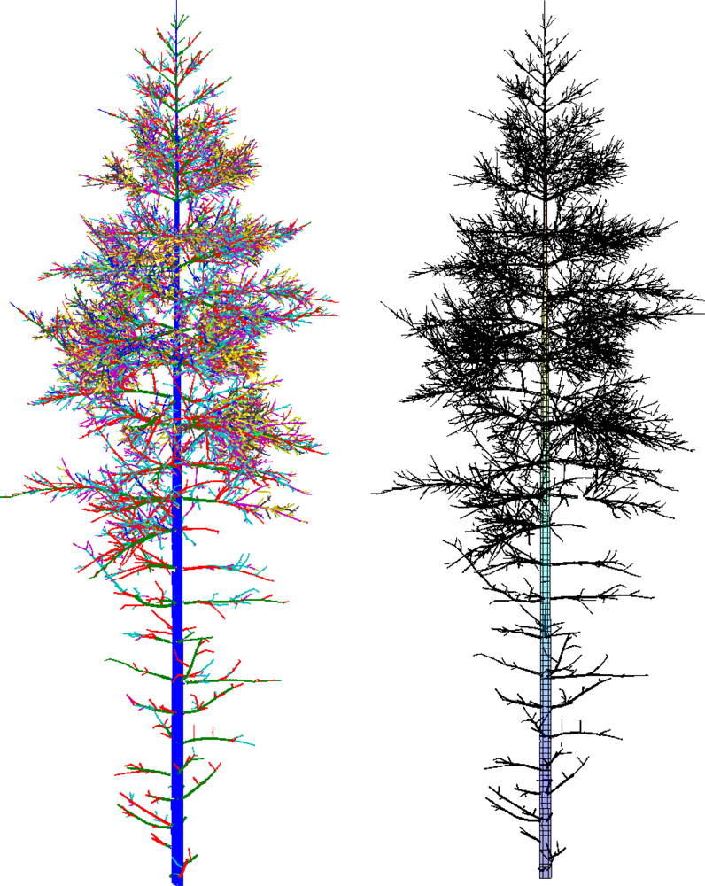
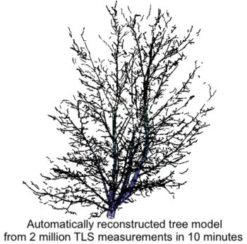
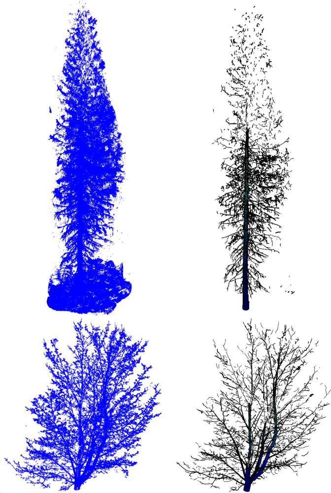
In this paper, we present a new method that produces 3D tree models from TLS data fulfilling all the conditions above (see the examples of reconstructed models in Figures 1 and 2). In particular, we present all the modeling steps from the point cloud data to a complete tree model. One of the core ideas behind the approach introduced here is that practically any external attributes of a tree can be approximated accurately at will from a compact model of the type above. The attributes can be, e.g., the volume and its distribution along different parts of the tree; the lengths and taper functions for the trunk and branches; the bifurcation frequency, topology and branching angles, a 3D “branch map”, etc. In this paper, we restrict the models to cover the woody parts of the tree (no foliage or needles), and only consider scans from a single tree.
Our scheme is based on the principle of building the global model step by step by an advancing collection of small connected surface patches. These patches are small local subsets of the point cloud and their geometric properties and neighbors are easily defined. This building-brick approach makes the method robust as the procedure does not need to know what a tree is supposed to look like and the point density can be quite varying. An ordered collection of local connected surface patches automatically yields the global structure both qualitatively and quantitatively.
A key part of any modeling method is the segmentation of the point cloud into branches. The segmentation gives the topological tree structure and the resulting segments (branches) can be then geometrically reconstructed. Our segmentation procedure uses the surface patches and recognizes bifurcations along the tree surface by checking local connectivity of a moving surface region. Other methods for segmenting have been presented: one way is to use voxels and mathematical morphology [21]. Another is to use octree based skeletonization approach [22,23]. Skeletons can be defined also using a neighborhood graph and checking the connected components of the level sets of the graph [17,24].
The paper is organized as follows. The method is presented in Section 2; in Section 2.1 we describe our data, and the outline of the method is given in Section 2.2. In Sections 2.3–2.10 we describe the method in detail, with some algorithmic points covered in the Appendix. In Section 3 we test the method using real and artificial TLS point clouds and show some results. Finally, Sections 4 and 5 contain discussion and conclusions.
We have published two short conference papers [25,26] describing some of the ideas of our method. In this paper, however, we develop the method further and present many more details, tests, and validations. The primary novel features of our method are: (i) the partition of the point cloud into patchlike sets that allow a fast automatic procedure; (ii) efficient segmentation rules that retain the topological and hierarchical information; and (iii) a tool-like interface with direct handles for any geometric and topological attributes of the tree. We render the processed point cloud of a tree in a readily accessible geometric mode that can be utilized by a wide variety of applications and end-users.
2. Method
2.1. Data: Point Clouds
A (laser scanner produced) point cloud PM is a finite subset of the 3-dimensional real coordinate space ℝ3. In this paper, each point x∈ PM gives the Cartesian x, y, z-coordinates of the corresponding scanned point. Furthermore, we assume that each point cloud PM is a sample of a surface M embedded in ℝ3. The surface M represents the surface of the scanned tree, and the point cloud PM is a finite but dense enough sample of M such that the point density varies little within distances of about the maximum trunk diameter. Notice also that the points in PM are unorganized and can be saved in any order as rows into a three-column matrix.
In this paper, we have used scans from four trees: one Norway spruce [Picea abies (L.) H. Karst] (see Figure 2), two Scots pines [Pinus sylvestris] (see the other in Figure 3), and one Norway maple [Acer platanoides] (see Figure 2). The trees were scanned from three different directions to have a comprehensive cover of the branching structure. The scans were registered to a common coordinate system via spherical reference targets placed in the measured area. Our method handles the TLS data only as point clouds and does not take into account the particular features of the equipment used. For the datasets used in this paper, our system consisted of a phase-based terrestrial laser scanner (Leica HDS6100 with a 650–690 nm wavelength). The distance measurement accuracy of the scanner is 2–3 mm, and the field-of-view is 360° × 310°, the circular beam diameter at the exit is 3 mm and the beam divergence is 0.22 mrad (see [9,27] for more details). The measured point clouds for the trees we have studied in this paper contain roughly one to five million points each. The horizontal distance of the scanner to the trunks and the point separation angle were about 7–12 m and 0.036 degrees, respectively. Thus the average point density on the surface of the trunk (at the level of the scanner) for a single scan is about 2–5 points per square centimeter.
We have also used a complex artificial tree model and simulated laser scanning to produce point clouds. This was done for controlled testing and validation of the method. The 3D structural tree model used here represents a 30-year-old Scots pine tree (see Figure 1 in this paper and Figure 4 in [28]). The model is generated using an empirical growth model parametrized by species-dependent branching statistics in conjunction with specified external environmental conditions [29]. TLS point clouds were simulated using the Monte Carlo ray-tracing code which has been used for a wide range of applications [28,30–32]. Simulation parameters were the same as in the scanner used in the measurements (see above). The simulated lidar was situated at 1.5 m height, at a radial distance of 20 m from the tree (at [0, 0, 0]), at 70°, 0° and −70° in the xy plane, i.e., xyz locations [0, 20, 1.5], [18.7939, 6.8404, 1.5] and [−18.7939, 6.8404, 1.5]. The simulated point cloud has about 4.5 million points.
2.2. Outline of the Method
Our method is based on covering the point cloud data with small sets corresponding connected patches on the tree surface. Then using a building-brick approach, the unknown global tree model is built by “growing” the tree surface step-by-step using the surface patches. After the patchwork over the tree has been obtained and the tree has been segmented into its branches, the remaining question is how to render it in a form suitable for fast computations and storage. The choice adopted here is the simplest one: the tree surface is reconstructed as an aggregate of small cylinders of varying size approximating parts of the trunk and branches. Cylinders (or their generalizations) are essentially a robust regularization choice that is sufficient for providing the essential attributes of the tree such as stem and branch diameters.
All the desired external characteristics of the tree can be readily approximated from the cylinder data. Moreover, the method is scale-independent because it uses only topological properties and relative sizes. Absolute size restrictions are related to cover set size (building brick size) and the accuracy and density of measurements. Thus, if the cover set size is small enough, the method can be used to reconstruct the model accurately down to the measurement accuracy of the laser scanning. From the point of view of information compression, the cylinder model retains most of the information of the original point cloud in a format that is hundreds to thousand times more compressed in size.
Constructing the tree model requires some assumptions and a priori knowledge about the data and trees. First, we assume that the point cloud is a locally uniform and extensive enough sample of the surface in a 3D Euclidean space modeling of the real tree. Second, it must be possible to cover the point cloud sample with small sets that correspond to connected patches along the surface. Third, some other features of the tree, such as the order of magnitude of the branch and trunk size and the approximate trunk direction, are assumed to be known. Finally, we assume the tree to be locally approximately cylindrical. In the future versions of the algorithm, we will include the option of deformable cylindrical surfaces whenever this approximation is significantly violated.
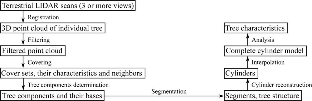
The main steps of the method are the following (see Figure 4). At first, the point cloud is filtered to remove noise or isolated points (see Section 2.3). Then the filtered point cloud is covered with small sets conforming to the surface of the tree (Section 2.4). Next the neighbor-relation of the cover sets is defined (Section 2.5) and the sets are geometrically characterized (Section 2.6). The neighbor-relation determines the connectivity properties, and the geometric characterizations are used, e.g., for the classification of trunk points. Next, the sets that are not part of the tree, such as the ground sets, are removed, and the tree components and their bases are defined (Section 2.7). Here, and throughout the paper, by a tree component we mean an essentially separate part or cluster of the point cloud that can be, e.g., a single branch, a collection of branches, or even the whole tree. Following this, the tree components are segmented (Section 2.8). Throughout the paper, by segment we mean a connected non-bifurcated part of the tree, such as a branch or part of a branch or the trunk. The segmentation also gives the ordered information of the tree structure. In the segmentation process, we use surface growing, and bifurcations are recognized by checking local connectivity. The next step is to approximate each segment as a sequence of cylinders of possibly varying radius, length, and orientation (Section 2.9). To complete the cylinder model of the whole tree, gaps between cylinders are sought and filled with additional cylinders (Section 2.10). Finally, statistical and other characteristics of the tree can be computed from the completed cylinder model (Section 3.1).
2.3. Filtering Noise from the Sample
The point cloud sample may contain outliers and noisy points caused by various reasons such as interference effects. Such points are not regarded as samples of the actual surface we want to reconstruct, and the first step in our method is to filter some noise from the point cloud. Our approach to filtering is based on the covers of the point cloud that are defined in the next section.
To remove separate single points or few-point clusters, we cover the point cloud with small balls and reject points that are only included in balls that contain fewer than some small number of points. A more comprehensive version of this filtering scheme is to define a small ball for each point and then reject the points whose balls contain too few points. The size of the balls and the number of points depend on the density of the points in the data. We have used balls whose radius is 1.5 cm and removed all the balls with less than three points.
Another, and possibly additional, filtering scheme to remove small separate parts of the point cloud uses covers of larger balls to determine the connected components of the point cloud. Then the points in components with too few cover sets are removed. We have used balls whose radius is 3 cm and removed all the components with less than tree balls.
The values of the filtering parameters and their effects on resulting tree models depend on the noise level and its distribution in the data, the geometry of the tree, etc., so there is no simple selection rule for the parameter values. However, we have found that, in practice, experience guides the selection of the values quite robustly. The effects are mainly local and usually not very sensitive to the parameter values. Furthermore, the same parameter values work well for similar trees and scanner parameters. For future versions of the algorithm, we will study automated machine learning of the parameter values and their adaptive adjustment.
2.4. Cover Sets
The embedding space ℝ3 is endowed with the usual Euclidean distance dis and thus Euclidean topology. The restriction disP of the distance dis to PM gives the distances between the points of PM, and thus also a metric topology for PM. Notice that disP locally approximates the distance function of the surface M and it can thus be used to approximate the surface M from the sample PM. A spherical neighborhood of radius r at x, or simply r-ball atx, is the subset B(x, r) of PM consisting of all the points y that satisfy disP (x,y) < r. A cover C = {Bi} of PM is a collection of subsets Bi ⊂ PM such that each point of PM belongs in at least one of the subsets Bi. A cover is a partition if each point belongs in exactly one of the subsets.
We aim to reconstruct the surface M from the sample PM, but the “global shape” and structures of M are impossible to determine directly from the whole sample. However, locally the surface and its structures can be approximated well from the sample. Furthermore, the sample PM is generally quite dense compared to the size of the local details of M. Therefore, a much smaller subsample of PM retains all the necessary information to reconstruct a cylinder model of the tree surface M. To accomplish these aims, we cover the sample PM with such small sets that they are expected to correspond to connected subsets of the surface (see Figure 5). Thus, the cover sets are small, connected surface patches and they define a new much smaller sample of M, which locally approximates the shape and topology of the surface. Because the cover sets are in a way the smallest unit sufficient to represent the sample PM, the size of the sets defines the limit of the details of M that can be accurately approximated (see Figure 6).
We generate two mutually related covers which are used for different purposes. First, we generate a cover CB = {Bi} of r-balls, which will then induce the other cover, a partition CP = {bi}. The cover CB is used to approximate the structures of M and to define the neighbor-relation for the partition CP, which is used to define the components and segments of the tree. The cover CB of r-balls is random, but to distribute the balls evenly along the surface, there are two restrictions: (1) the minimum distance between the centers of two balls is d; and (2) the maximum distance from any point to the nearest center is also d. The parameter d is a little smaller than, or equal to, the radius r, and it controls the size of the cover sets in the partition CP. The partition CP = {bi} is induced by the r-balls: for each ball Bi there is a corresponding set bi that consists of those points of Bi that are closer to the center of Bi than any other center. Thus the minimum diameter of the sets bi, in the case they are not near, e.g., the tip of a branch, is d and the maximum possible diameter is 2d.
The parameters d and r should be as small as possible so that the cover sets conform to the details of the surface. On the other hand, they should be large enough so that the sets can be reliably used to approximate different characteristics, such as surface normals, and to restrict the computational requirements. The parameters depend on the size of the smallest branches/details we are looking for, the point density, and the noise level. Usually, in the case of trees, d is about 1 to 3 cm. To generate the r-balls, we first partition PM into cubes with side length r. Then each r-ball belongs to the r-cube containing the center and the 26 neighboring cubes.
2.5. Neighbor-Relation
The neighbor-relation for the partition CP is a central tool defined by the r-balls: Let bi and bj be cover sets of the partition CP, and Bi and Bj be the corresponding r-balls. Then bi and bj are neighbors, if either bi and Bj or bj and Bi have a common point. Thus, the smaller d is compared to r, the more neighbors there possibly are for each cover set in CP. To guarantee that cover sets whose centers are up to 2d apart from each other are neighbors, as they should, r should be little larger than d. Notice also that the number of neighbors varies and thus a natural way to store the neighbor information is to use cell-arrays with variable cell size.
Let G be a cover set or a group of cover sets. With the neighbor-relations, G can be extended by adding its neighbors to it, and the resulting group of cover sets is denoted by Ext(G). This can be repeated multiple times and we can, e.g., “grow” the tree surface from the given initial set and thus also change the scale from small to large.
One of the applications of the cover set extension is to determine connected components or connectedness of a given group of cover sets: two cover sets of CP are in the same component if the cover sets can be expanded by the neighbor-relation to the same sets. Furthermore, the maximal disjoint sets generated by the cover set extension are the connected components of a given group of cover sets.
2.6. Characterization of Subsets
Next, we present a number of useful geometric characterizations of the cover sets and other subsets B ⊂ PM of the point cloud. Many of these use the eigenvectors and eigenvalues of the structure tensor (i.e., scatter matrix or covariance matrix) S(B) of B[33]: Let {u1,u2,u3} be the unit eigenvectors of S(B) such that the corresponding eigenvalues satisfy λ1 ≥ λ2 ≥3.
If B is a r-ball, then {u1,u2} span the tangent space and u3 approximates the normal line (u3 can point to either side of the surface M) [34]. The eigenvectors also give the principal components of the set B, i.e., they describe the orthogonal components of the data exhibiting maximal variance [35]. The eigenvalues of S(B) can be used as indicators for the dimensionality of the set B[36], i.e., if the set is elongated, planar or 3-dimensional.
We use the eigenvectors S(B) also to define the branch direction line D(B) for each r-ball B as a unit vector that estimates the direction of the underlying branch or trunk at B. For clearly elongated sets we set D(B) equal to u1. For other sets we use the normals of B and its neighboring sets to define D(B). Because branches are locally approximately cylindrical, the normals of the neighboring sets are all approximately orthogonal to the branch direction. Thus the vector that minimizes the sum of the squared dot products with the normals is a good approximation of the branch direction. Then D(B) is the unit eigenvector corresponding to the smallest eigenvalue of the matrix NTN, where N is the matrix whose rows are the unit normals of B and its neighbors.
For many trees, the trunk, at least near the base of the tree, is often almost straight and has generally a direction different from that of the most branches and the nearby ground. Thus, if the trunk direction can be estimated (globally) by a vector T, then the angle between T and D(B) estimates the parallelism of the underlying branch/trunk of a cover set B.
2.7. Tree Components and Their Bases
The next step, after the generation of a cover, the determination of its neighbor-relation, and the geometric characterization of its sets, is to extract the cover sets pertaining to the tree. In other words, the point cloud may contain ground and other points which are not part of the tree. These parts are removed and the base of the trunk is defined. Furthermore, because of possible gaps in the data, the point cloud may have multiple (often hundreds or thousands) connected components of the tree. The bases of these other tree components also need to be defined because later on, starting from the base each component is segmented into its branches. Although we next present an automatic way to separate the surroundings from the tree, we still assume that the tree is the only (big) tree in the point cloud. Hence the manual removal of adjacent trees from the point cloud may be needed. An automated way to handle multiple trees is a subject of future development.
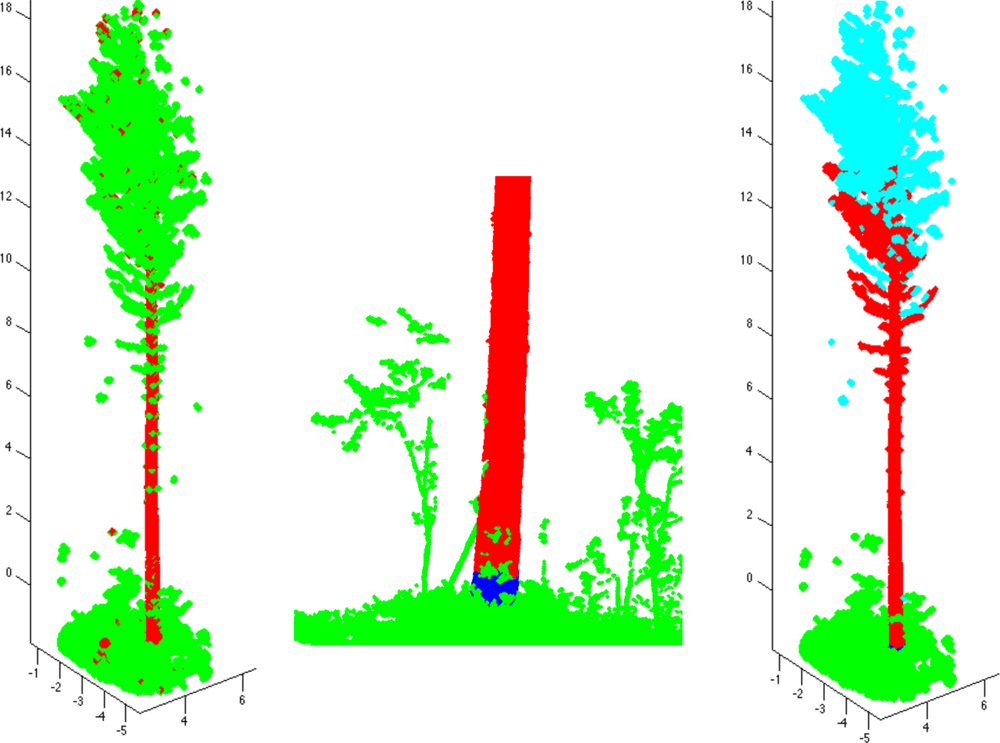
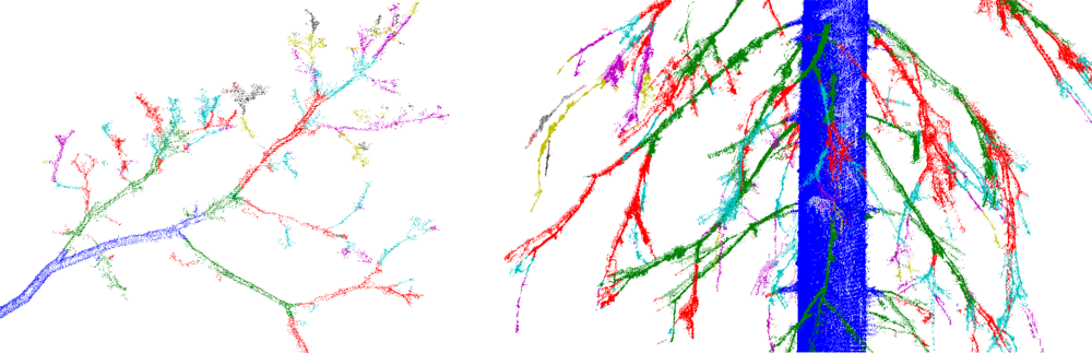
To determine the tree components, the trunk is first defined approximately as a set Trunk of all those cover sets that are parallel to the approximated trunk direction and are two-dimensional (see also [9,25]). Next redefine the trunk by including its neighboring cover sets, i.e., set Trunk = Ext(Trunk). On the left in Figure 3, we show an example of set Trunk so defined. The set Trunk may contain small branch components and parts of ground, but most of these can be easily removed by determining the connected components of Trunk and then removing all the small components. Furthermore, using the largest component of Trunk, the axis of the trunk can be estimated and Trunk can be redefined as those large components whose mean is less than, say, half a meter away from the axis.
Next, define the base TBase of the trunk as the lowest part (and its neighbors) of the lowest component of Trunk (e.g., a 20-cm slice from the lowest point). Most of the ground and other sets that are not part of the tree can now be removed easily. First, define the set Ground containing the cover sets connected to the tree base TBase, but not connected to it through Trunk. The set Ground now includes ground and vegetation points. Next, define the tree component starting from TBase by expanding TBase as long as possible, but prevent the expansion into Ground. This is now the first tree component and TBase is its base (see the middle frame of Figure 3).
Next, determine the connected components of the point cloud from which Ground and the first tree component are removed. Then find out which of these components are part of the tree. This can be done heuristically by defining the means of the components and then checking their heights from the ground and distances to the trunk axis. The final classification of the connected components is shown in the last frame of Figure 3.
The bases of the other tree components need to be determined for the segmentation process. There is no easy and fast way to do this with full reliability, and for some components, the defined base may not be the right one. A wrong base can mix up the branching-relation, i.e., which segment is the parent branch and which is the child branch. However, our heuristic apparently works most of the time. If the component shares common sets with Trunk, then we select the lowest common set as its base, and this base defines a trunk segment. For other components, we first project the component into its largest principal component to find its two ends in the principal direction. Then, we select the end that is closer to the trunk axis as the base of the component.
2.8. Segmentation
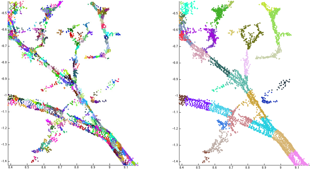
When the tree components and their bases are determined, the next step is to segment these components into branches. Each component is partitioned into segments that correspond to the whole or part of a real branch or trunk. In particular, segments should not have any bifurcations. This kind of segmenting also defines the tree structure, i.e., the branching-relations of the child and parent branches for each branch. It is also straightforward to fit cylinders to these segments. Examples of segmented tree parts are shown in Figure 7 and Figure 1 shows a segmented tree.
2.8.1. Overview of the Algorithm
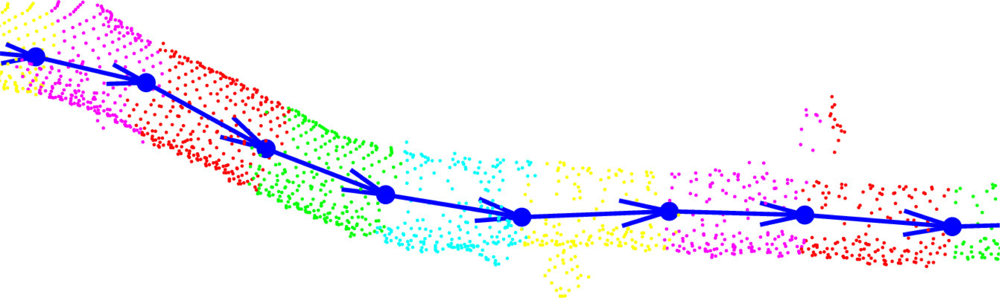
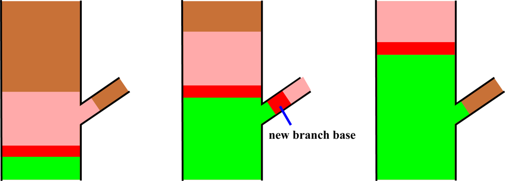
The segmentation process takes place at the level of the cover sets, and the basic tool is their neighbor-relation. The procedure starts from the base of a tree component and, step by step, a cut region and its extension, a study region, move along the component (see Figure 8). The cover sets are the building bricks of the tree surface and the cut region is a layer of these bricks that separates the component into two parts. At each step the cut region moves to the neighboring layer of cover sets. Every cut region is expanded or “grown” along the tree component into the study region that consists of multiple layers of cover sets. Each study region is checked for connectivity to find out possible bifurcations. If the study region is not connected, then it is further checked if its separate parts are the beginnings of new branches or parts of the current segment. The part of the cut region in a branch becomes a base for a new segment to be determined later. The parts of the cut region that are not new segment bases are added to the segment, and this way the segment grows one layer a time. The segment is expanded until no cut regions can be constructed or none of the separate parts of the study region are clear continuations of the segment. A schematic picture of this process is shown in Figure 8.
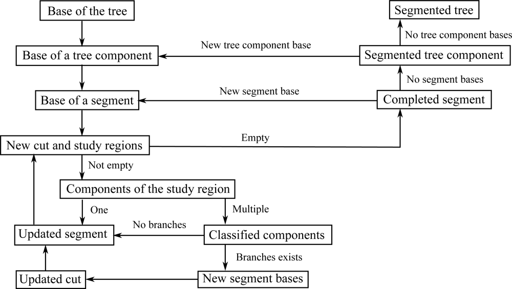
Notice that each new segment base found also defines the tree structure step by step. Furthermore, because only neighbor-relations and relative sizes are needed, the process is scale independent. However, the accuracy and density of the scanned data points and the size of the cover sets define a limit for the separation: If the accuracy of the scanned points is of the order of the width of the gap between neighboring parallel branches, then the two branches are merged into one in the data. Also, if the density of the points is so small that the distance between the closest points is about the same as the gap between branches, then the gap and thus the branches are indistinguishable. Finally, if the branches are so small that they are contained (in the transversal direction) in a single cover set, they are also indistinguishable, because segments are collections of cover sets. Figure 9 shows the segmentation process as a flow chart. Details of the segmentation algorithm are given in the Appendix.
2.8.2. Remarks
Because each segment is constructed one layer of cover sets at a time, these layers partition the segments. These layers should be saved so that they can be used in the cylinder reconstruction, where the segments are first divided into smaller regions. Furthermore, especially in the trunk where the cover sets are small compared to the segment size, gaps in the data due to self-shadowing may lead to wrong segments. These gaps may lead to small segments along the trunk which are classified as child segments of the trunk segment that continues past them, i.e., the child and parent segments are part of the same real trunk at the same height of the trunk. When cylinders are fitted to these small segments, the cylinders are strongly overlapping and nearly parallel to the cylinders in the parent trunk segment. This can be corrected by comparing the cylinders in these segments and removing the overlapping ones in the child segments.
2.9. Cylinder Reconstruction
Each segment is reconstructed with successive cylinders locally approximating the radius and orientation of the segment (branch). In the process, also the succession relations of the fitted cylinders are recorded so that the tree structure can be expressed in terms of the child/parent relation of the cylinders.
The cylinders are expressed parametrically with seven real numbers (the radius and the components of the axis direction vector and the axis position vector) and the parameters are optimized using the total least squares method [37]. This nonlinear optimization problem requires iterative solution methods with good initial estimates for the parameter values [38]. Another possible way to fit cylinders is to fix the axis direction and project the points into a plane orthogonal to the axis. Then we fit a circle to the projected points in the least square sense [39].
Our adopted approach starts from the base of a segment and then subdivides it into small successive pieces. These pieces consist of layers of cover sets and, here, the partition of the segment into layers in the segmentation process can be used. The number of layers should be such that the length of the pieces is at least equal to the estimated diameter of the segment. The center points of the successive pieces define vectors that define the regions, which are later approximated with cylinders. The regions form a new subdivision of the segment and each region consists of those points of two consecutive pieces whose projected points are between the start and end points of the vector joining the center points of the pieces (see Figure 10). These vectors and their starting points are also used as the initial estimates for the axis direction and starting point in the cylinder fitting. The initial estimate for the radius can be the mean or median distance of the points in the region from its estimated axis. Longer regions are more tolerant of noise, outliers, and imperfect point cover, but in some cases, they may not follow the radius and direction of the branch as accurately as shorter regions. The effects of outliers and noise can also be reduced by a second fitting: the cylinder of the first fitting is used to identify points far away from the cylinder that can be removed from the point set of the second fitting.
When all the regions of a segment are approximated by an adjusted sequence of cylinders, the radii of the cylinders are checked using prior knowledge: the diameter of a branch is practically always smaller or only a little larger than the diameter of its parent, and the diameter of a branch usually decreases away from its base. Moreover, to make the sequence more continuous (e.g., to close small gaps between the cylinders) and to correct for the effects of radius changes, the starting points and the axes are modified when needed.
2.10. Completing the Cylinder Model
When all the segments are reconstructed with cylinders, the cylinder model may still be refined. The point cloud may have multiple connected components, in which case there are gaps between these components. There may also be clear gaps between a parent cylinder and its child cylinder which is not an extension. Thus there may be gaps in the cylinder model which can produce errors for the tree statistics. To reduce these errors, we identify small gaps between the fitted cylinders and then fit cylinders to these gaps using only the previously fitted cylinders as data.
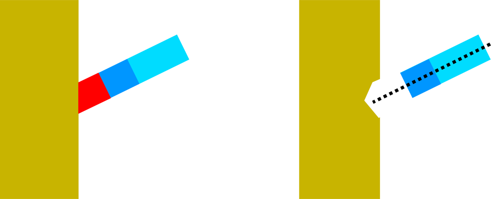
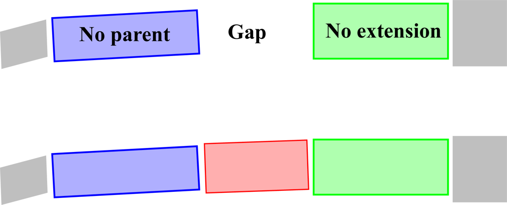
There are two basic cases. In the first case, there are two nearby and nearly parallel cylinders, one without a parent (C) and the other without an extension (A) (see Figure 11). Define a vector from the top of A to the bottom of C. Then this vector defines the axis of the new cylinder B whose radius is the mean of the radii of A and C. Moreover, B not only joins the cylinder chains but also the underlying segments since the segments of A and C are joined into one single segment. In this way, the tree structure is also refined.
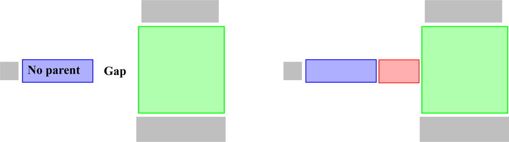
In the second case, there is a cylinder C without a parent, and, close to it, there is a second cylinder A which is transversal to C and has larger radius (see Figure 12). The idea is to add a new cylinder B as a child of A such that the radius of B equals that of C. Furthermore, the axis line of B will intersect the axis of A, and the axes of C and B are adjusted to be as parallel as possible. Again, the added cylinder refines the tree structure.
3. Testing and Results
In this section we first define different tree metrics that can be approximated from completed tree models. Then we test our method using first simulated TLS data from artificial tree models. Next, we compare model results for caliper measurements of small branches of a real tree. Finally, we present complete models and results for real trees.
3.1. Tree Metrics
A large variety of (external) statistical measures and other characteristics of the tree can be approximated from the cylinder model. These are, e.g., the total volume of the whole tree or its parts such as the part of trunk with certain radii and the branches of certain size. The total volume and length of the trunk and branches can be also estimated, but depending on the quality of data (e.g., the extent of surface cover), the upper parts of the tree may be quite incomplete. Similarly, the sum of the lengths of the cylinders gives a good estimate of the total branch length in the tree. Trunk and branch profiles (taper functions) can also be easily estimated.
There are other statistical data that can be approximated from the cylinder model, e.g., the number of sub-branches originating from branches, the angles between child and parent branches, and the averages of these. An important concept is the branch size distribution, which characterizes a tree in many ways. From the cylinder models we determine the distribution as follows: we assign the branch cylinders according to their diameter into bins (under 1 cm, over 1 cm but under 2 cm, over 2 cm but under 3 cm, etc.). and then compute how much of the total branch volume there is in each bin.
3.2. Testing with Artificial Trees
The basic performance of the procedure for the parts existing in the data was validated in [40], where random but uniformly distributed samples were taken from a simple artificial tree. Random samples mimicking typical target sizes estimated the error level to remain within the expect bounds; i.e., within roughly 5–10% for the characteristics of the whole part existing in the data, depending on the reconstructed quantity.
To test the method with more realistic data and the dependency of some results on the main input parameters, the cover parameters d and r, we have used simulated TLS scanning from a complex artificial 3D tree model (see Section 2.1). First, we fixed the cover set diameter d to 2.0 cm and checked how changes in the radius r, which controls the geometric characteristics and neighbor-relation, affect reconstructions. The resulting partition CP was the same for each case. The results for the radius test are shown in Table 1. Figure 1 shows the segmented point cloud and the final cylinder model when d = 2.0 cm and r = 2.4 cm.
Obviously, as the radius increases, the connectivity increases as well, which is reflected in the decreasing number of tree components. We also see that the total branch length and the number of branches are little affected by the increasing radius, but they decrease somewhat. This is again expected because of the increasing connectivity (larger neighborhoods). Because there are about 1,778 m of branches with a diameter under 1 cm in the original tree, it is clear that not all of them are sampled sufficiently by the point cloud. This explains the difference between the total branch lengths of the original and reconstructed. Nearly all or all the first-order branches (branches originating from the trunk) are found, and with a larger radius also some second-order branches very close to trunk are classified as first-order branches. The evaluation of the branching structures beyond the first order is complicated because there are lots of separate components and the order of the “base branch,” even if that exists, is unknown. However, visual inspection verifies that the branching structure is well defined inside the components in the sense of branch separation. We also see that, for a large radius, the trunk classification, due to, e.g., the segmentation and initial trunk component classification, varies quite a lot in the sense of trunk length. However, most of the trunk volume is still covered as the length differences pertain to thin parts. From the data we conclude that in this case the suitable radius r is about 2.0–2.4 cm, and thus the radius can be a little larger than the diameter d.
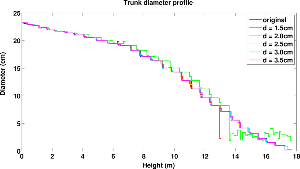
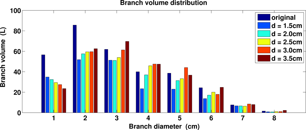
Next we used multiple different sizes for cover sets to see the effect of the diameter d on the results (in each case the radius is 0.4 cm larger than the diameter). Figure 13 shows that the trunk profiles of the original and reconstructed trees are little affected by the size of the cover set, except for small variations in the upper part for the smallest cover sets (see also the trunk volumes in Table 2). This is expected because most of the trunk is visible in the data and it is covered quite well all around. Figure 14 shows the branch size distribution of the original and reconstructed trees. First, only part of the smallest branches (diameter under 2 cm) exists in the data and thus only part of their volume is reconstructed. Second, branches whose diameters are much smaller than the cover set usually cannot be sharply segmented. Then a large cover set may contain points from multiple nearby small branches or from a branch and its child branches. Thus we see that the larger the cover sets, the larger the bins in the volume distributions and the less the number of branches and components. This can be seen also in Table 2: the total volume and length of the branch cylinders increase and decrease, respectively, as d increases. When the trunk is correctly defined, then all (or nearly all) first-order branches are found, and with larger d few second-order branches close to trunk are classified as first-order branches. Again, the branching structure is well defined for most of the tree, and the differences are in the smallest branches.
3.3. Testing with Real Measurements for Small Branches
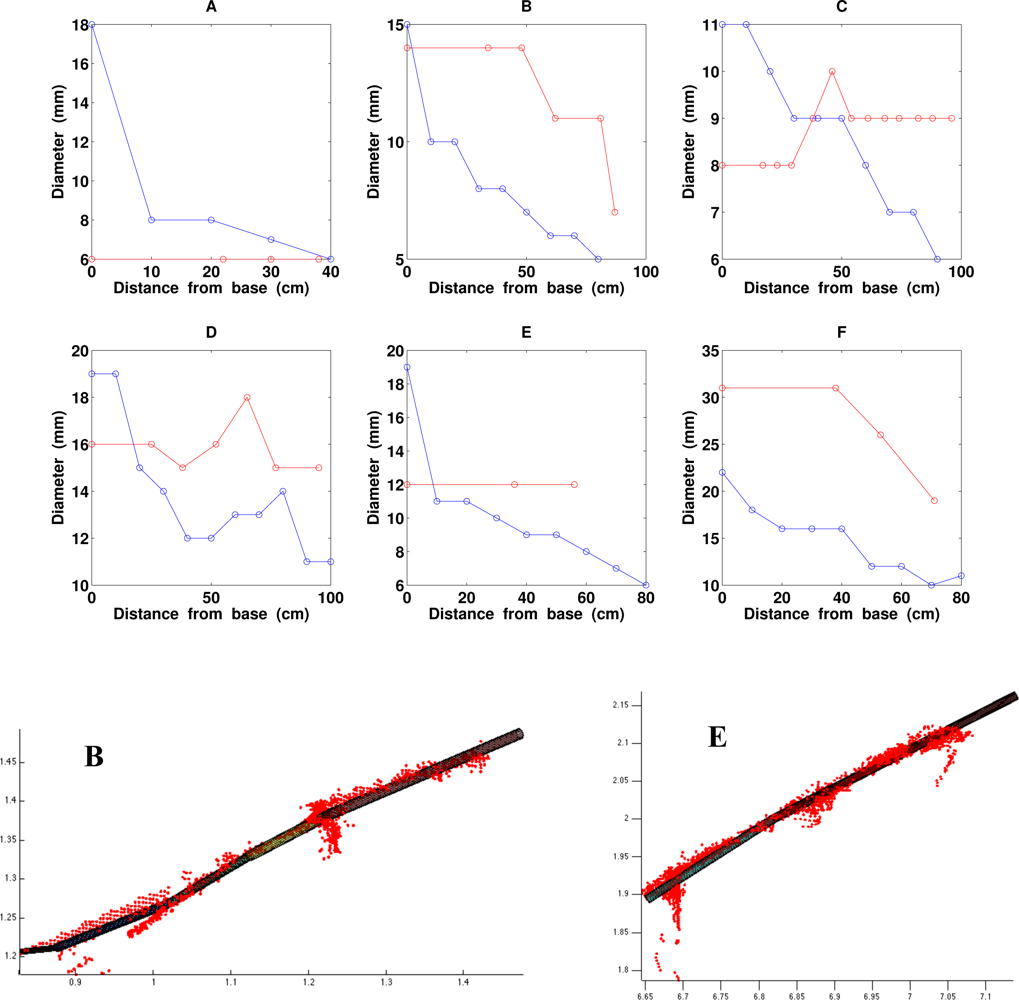
There are many sources of errors in the scanning, particularly for small branches. The size of the laser spot is about 5 mm when it hits the branch (the spot size depends on the distance). There is also a small error when scans from different directions are registered into a common coordinate system (some millimeters). Windy conditions can add some error due to movement of the branches. Furthermore, the scanning beam can be reflected from parts outside the actual surface. For example, there is a certain amount of data noise in coniferous trees throughout the year due to needles. Thus, it is clear that the smallest branches (diameter under 3 cm) cannot be scanned very accurately. In order to check if the cylinder reconstruction works at all for branches whose diameter is near the scanning accuracy, we have measured some branch profiles for the spruce shown in Figure 2 using caliper. The branches have small diameters (about 1–3 cm) and their height above the ground is some 1–3 m. In Figure 15, we show some caliper measurement results and compare them with the results obtained from the cylinder model.
Assuming that the caliper measurements are accurate, the results show that the diameter measurement error for very small branches is of the order of one centimeter, and usually the computed diameter is larger than the measured one. There may, of course, be different biases in the two measurements (caliper and cylinders) which affect the results. For example, the cross-section of small branches is rarely circular. However, the accuracy of the cylinder fitting for branches whose diameter is near the scanning accuracy is as expected. Moreover, the orientations and locations of branches and the tree structure can still usually be reliably reconstructed for small branches, as can be seen from the bottom frames of Figure 15.
3.4. Complete Models from Real TLS Data
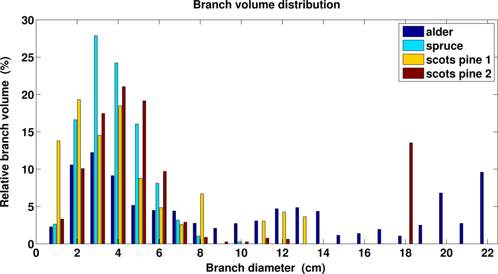
We have scanned four trees, a Norway spruce and maple, and two Scots pines, the first one shown in Figure 3. The trees have been scanned from three different directions to have a comprehensive cover of the branching structure (see the scanner specifications in Section 2.1). Complete cylinder models for a Norway spruce and maple (without leaves) are shown in Figure 2. In Table 3, we show some statistics computed for the trees. Branch size distributions for the trees are shown in Figure 16. Notice that because the trunks of the maple and the scots pine 2 bifurcate, a significant proportion of the branch volume is in large branches with diameter over 10 cm.
4. Discussion
The results from Section 3 demonstrate that our method is able to automatically build models that reconstruct the parts existing in the data. With near-perfect data, such as the simulated data, where potential error sources (registration, wind, etc.) can be controlled and eliminated, the method is able to reconstruct the tree accurately. Even small branches near the accuracy level of scanning can be reconstructed, and their branching structure is retained in the model. Overall, the results seem quite good and, e.g., trunk volumes are very close to the real ones. Compared to a recent voxel-based method [41], where there was much better cover of the tree (4–5 scanning positions and 20–60 million points) and smaller unit size (1 cm), the errors in the total volume are about the same. In future studies, we plan to conduct more validation tests with large field measurements.
Most of the parts missing in the data are not reconstructed, and this affects different tree metrics estimated from the model. In particular, the top parts of (high) trees are usually poorly covered by TLS data (see Figure 2). However, because the lower parts have a better cover, it should be possible to use the modeled lower parts to give accurate corrections to the total volumes and branch size distributions in the upper parts. This is a subject for further study.
The method does not model the foliage or needles, and if these are present, they can add noise, make nearby branches indistinguishable, prevent the visibility of many parts, etc. Needles, especially, can make the smallest branches appear larger in diameter then they are. Again, however, these could be taken into account with proper calibration, but this requires extensive field measurements and testing.
The segmentation works well and the separation of the branches comparable or larger in sizes to the cover sets is nearly perfect. Large noise, if it cannot be properly removed, can affect the separation of branches but this cannot be helped. Thus individual branches can be analyzed and their topological relation to the other branches can be determined. However, gaps in the data breaks the data into separate components and the relations of the components is harder to determine accurately. The gap-filling procedure presented in Section 2.10 was realized so that only very clear cases were allowed. Thus, only a few tens of gaps were filled in any of the reconstructed models. This procedure will be developed further.
As shown in Section 3.2, the method is quite robust against the selection of the cover parameters d and r. This is especially true for parts that are large enough compared to d; i.e., when the sampling size is small enough, the reconstruction works well. However, this method and all methods reconstructing the whole tree structure from point clouds are quite sensitive to the quality of the measurements. Therefore, for example, if the point density is too low or there is lot of movement in the tree during the measurements, the smallest branches cannot be reliably reconstructed.
We have implemented the method with MATLAB, and the main inputs are the point cloud as well as the cover and filtering parameters. Other parameters determine, e.g., if a component is part of the tree, whose parts are initially classified as trunk, and converge criteria for cylinder fitting. If these parameters are approximately tuned, the method is automatic and no human intervention is needed. The computation time and memory required mainly depend on the number of cover sets used, and for most of the steps, the time depends linearly on the number of sets. Especially for the segmentation, which is the most time-consuming step, the required time is roughly proportional to the total length of the branches. However, the time and hardware requirements are modest; the whole process (with data sets of 1–5 million points) takes from minutes to half an hour (see the tables in Section 3) with a MacBook Pro (2.8 GHz, 8 GB).
In future work, we will apply our method to a larger number of trees to draw some statistical inferences, and we will analyze exposed stumps and roots of trees, for which there is so far very little size and structure data (Liski et al., in preparation). We will also compare the results obtained with conical-elliptic shapes and deformable cylinders to estimate the inherent systematic errors of the procedure in some attributes extracted. Furthermore, the computational method and its realizations still need some testing, validations, and further developments, such as adaptive parameter tuning, so that a general software package can be compiled for a variety of end-users.
5. Conclusions
We have presented the main steps and demonstrated the potential and operability of a method for constructing automatically comprehensive precision models of trees from TLS point clouds. The method is fast, producing almost immediately a model that is compact compared to the measurement data. In the model, the diameters and orientations of the trunk and branches are locally approximated with cylinders. The branching structure, i.e., the parent–child relation of the branches, is also recorded in the model. The method is independent of the absolute scale and can thus be used to analyze the tree quantitatively down to the level of detail allowed by the data.
The cover-set approach is the driving engine behind our method. It renders the point cloud as a collection of topologically, geometrically, and hierarchically defined units that can be analyzed with standard fitting procedures to obtain orientations, sizes, etc. The other key principle presented here is the wholesale processing of the point cloud to obtain a simple easily accessible model that is designed to contain most of the necessary trunk–branch information even without defining that information a priori.
Using the model, we can carry out quantitative analysis of the structure and size properties of the tree. For example, the total volume of the whole tree or any of its parts, such as the trunk or branches, can be approximated from the model. The trunk and branch profiles, or statistical distributions such as the branching angle distribution, can be determined from the model. In particular, the model yields the branch size distributions, which can be used to improve tree quality and forest carbon cycle estimations.
The reference measurements from small real tree branches show that the method is able to reconstruct the branches with reasonable accuracy (error under 1 cm). The results from the modeled TLS data show that the volume of trunks and large branches can be reconstructed accurately (few percent error) even when large portions of tree parts are not sampled by measurements. The data need not be as comprehensive and dense as required for voxel-based methods.
In the future, we will validate the method further with a large number of trunk and branch measurements from real trees. We will also develop the method further, e.g., by utilizing generalized cylinder shapes.
Together with the computational method presented, laser scanning provides a fast and efficient means to collect essential geometric and topological data from trees, thereby substantially increasing the available data from trees.
Acknowledgments
This study was financially supported by the Academy of Finland projects: Modelling and applications of stochastic and regular surfaces in inverse problems and New techniques in active remote sensing: hyperspectral laser in environmental change detection, and the Finnish Centre of Excellence in Inverse Problems Research. We thank Jari Liski and Risto Sievänen for valuable discussions and suggestions.
References
- Peuhkurinen, J.; Maltamo, M.; Malinen, M.; Pitkänen, J.; Packalén, P. Preharvest measurement of marked stands using airborne laser scanning. For. Sci 2007, 53, 653–661. [Google Scholar]
- Repola, J. Biomass equations for Scots pine and Norway spruce in Finland. Silva Fennica 2009, 43, 625–647. [Google Scholar]
- Van Leeuwen, M.; Nieuwenhuis, M. Retrieval of forest structural parameters using lidar remote sensing. Eur. J. For. Res 2010, 129, 749–770. [Google Scholar]
- Dassot, M.; Constant, T.; Fournier, M. The use of terrestrial LiDAR technology in forest science: Application fields, benefits and challenges. Ann. For. Sci 2011, 68, 959–974. [Google Scholar]
- Hyyppä, J.; Jaakkola, A.; Hyyppä, H.; Kaartinen, H.; Kukko, A.; Holopainen, M.; Zhu, L.; Vastaranta, M.; Kaasalainen, S.; Krooks, A.; et al. Map Updating and Change Detection Using Vehicle-Based Laser Scanning. Proceedings of 2009 Urban Remote Sensing Joint Event, Shanghai, China, 20–22 May 2009.
- Holopainen, M.; Vastaranta, M.; Kankare, M.; Räty, M; Vaaja, M.; Liang, X.; Yu, X.; Hyyppäa, J.; Hyyppä, H.; Viitala, R.; et al. Biomass estimation of individual trees using stem and crown diameter TLS measurements. Int. Arch. Photogramm. Remote Sens. Spat. Inf. Sci 2011, 38, 91–95. [Google Scholar]
- Henning, J.G.; Radtke, P.J. Detailed stem measurements of standing trees from ground-based scanning lidar. For. Sci 2006, 52, 67–80. [Google Scholar]
- Hopkinson, C.; Chasmer, L.; Young-Pow, C.; Treitz, P. Assessing forest metrics with a ground-based scanning lidar. Can. J. For. Res 2004, 34, 573–583. [Google Scholar]
- Liang, X.; Litkey, P.; Hyyppaä, J.; Kaartinen, H.; Vastaranta, M.; Holopainen, M. Automatic stem mapping using single-scan terrestrial laser scanning. IEEE Trans. Geosci. Remote Sens 2012, 50, 661–670. [Google Scholar]
- Pfeifer, N.; Gorte, B.; Winterhalder, D. Automatic reconstruction of single trees from terrestrial laser scanner data. Int. Arch. Photogramm. Remote Sens. Spat. Inf. Sci. 2004, 35(B5), 114–119. [Google Scholar]
- Thies, M.; Pfeifer, N.; Winterhalder, D.; Gorte, B.G.H. Three-dimensional reconstruction of stems for assessment of taper, sweep and lean based on laser scanning of standing trees. Scand. J. For. Res 2004, 19, 571–581. [Google Scholar]
- Watt, P.J.; Donoghue, D.N.M. Measuring forest structure with terrestrial laser scanning. Int. J. Remote Sens 2005, 26, 1437–1446. [Google Scholar]
- Moorthy, I.; Miller, J.R.; Hu, B.; Chen, J.; Li, Q. Retrieving crown leaf area index from an individual tree using ground-based lidar data. Can. J. Remote Sens 2008, 34, 320–332. [Google Scholar]
- Pfeifer, N.; Winterhalder, D. Modelling of tree cross sections from terrestrial laser-scanning data with free-form curves. Int. Arch. Photogramm. Remote Sens. Spat. Inf. Sci 2004, 36, 76–81. [Google Scholar]
- Binney, J.; Sukhatme, G.S. 3D Tree Reconstruction from Laser Range Data. Proceedings of ICRA ’09 IEEE International Conference on Robotics and Automation, Kobe, Japan, 12– 17 May 2009; pp. 1321–1326.
- Bucksch, A.; Fleck, S. Automated detection of branches dimensions in woody skeletons of fruit tree canopies. Photogramm. Eng. Remote Sensing 2011, 77, 229–240. [Google Scholar]
- Côté, J.-F.; Widlowski, J.-L.; Fournier, R.A.; Verstraete, M.M. The structural and radiative consistency of three-dimensional tree reconstructions from terrestrial lidar. Remote Sens. Environ 2009, 113, 1067–1081. [Google Scholar]
- Filin, S.; Pfeifer, N. Neighborhood systems for airborne laser data. Photogramm. Eng. Remote Sensing 2005, 71, 743–755. [Google Scholar]
- Maas, H.-G.; Bienert, A.; Scheller, S.; Keane, E. Automatic forest inventory parameter determination from terrestrial laser scanner data. Int. J. Remote Sens 2008, 29, 1579–1593. [Google Scholar]
- Rutzinger, M.; Pratihast, A.K.; Oude Elberink, S.; Vosselman, G. Detection and modeling of 3D trees from mobile laser scanning data. Int. Arch. Photogramm. Remote Sens. Spat. Inf. Sci 2010, 38, 520–525. [Google Scholar]
- Gorte, B.G.H.; Pfeifer, N. Structuring laser scanned trees using 3D mathematical morphology. Int. Arch. Photogramm. Remote Sens. Spat. Inf. Sci 2004, 35, 929–933. [Google Scholar]
- Bucksch, A.; Lindenbergh, R. CAMPINO—A skeletonization method for point cloud processing. ISPRS J. Photogramm 2008, 63, 115–127. [Google Scholar]
- Bucksch, A.; Lindenbergh, R.; Menenti, M. SkelTre-Robust skeleton extraction from imperfect point clouds. Vis. Comput 2010, 26, 1283–1300. [Google Scholar]
- Verroust, A.; Lazarus, F. Extracting skeletal curves from 3D scattered data. Vis. Comput 2000, 16, 15–25. [Google Scholar]
- Raumonen, P.; Kaasalainen, S.; Kaasalainen, M.; Kaartinen, H. Approximation of volume and branch size distribution of trees from laser scanner data. Int. Arch. Photogramm. Remote Sens. Spat. Inf. Sci. 2011, 38(5/W12), 79–84. [Google Scholar]
- Åkerblom, M.; Raumonen, P.; Kaasalainen, M.; Kaasalainen, S.; Kaartinen, H. Comprehensive Quantitative Tree Models from TLS Data. Proceedings of 2012 IEEE International Geoscience and Remote Sensing Symposium (IGARSS), Munich, Germany, 22– 27 July 2012; pp. 6507–6510.
- Kaasalainen, S.; Jaakkola, A.; Kaasalainen, M.; Krooks, A.; Kukko, A. Analysis of incidence angle and distance effects on terrestrial laser scanner intensity: Search for correction methods. Remote Sens 2011, 3, 2207–2221. [Google Scholar]
- Disney, M.I.; Lewis, P.; Saich, P. 3D modelling of forest canopy structure for remote sensing simulations in the optical and microwave domains. Remote Sens. Environ 2006, 100, 114–132. [Google Scholar]
- Leersnijder, R.P. PINOGRAM: A Pine Growth Area Model, WAU Dissertation 1499. Wageningen Agricultural University, Wageningen, The Netherlands, 1992.
- Disney, M.I.; Lewis, P.; Gomez-Dans, J.; Roy, D.; Wooster, M.; Lajas, D. 3D radiative transfer modelling of fire impacts on a two-layer savanna system. Remote Sens. Environ 2011, 115, 1866–1881. [Google Scholar]
- Widlowski, J.-L.; Robustelli, M.; Disney, M.I.; Gastellu-Etchegorry, J.-P.; Lavergne, T.; Lewis, P.; North, P.R.J.; Pinty, B.; Thompson, R.; Verstraete, M.M. The RAMI Online Model Checker (ROMC): A web-based benchmarking facility for canopy reflectance models. Remote Sens. Environ 2008, 112, 1144–1150. [Google Scholar]
- Hancock, S.; Lewis, P.; Foster, M.; Disney, M.I.; Muller, J.-P. Measuring tree height over topography and understory vegetation with dual wavelength lidar: A simulation study. Agric. For. Meteorol 2012, 161, 123–133. [Google Scholar]
- Bae, K.-H.; Lichti, D.D. A method for automated registration of unorganised point clouds. ISPRS J. Photogramm 2008, 63, 36–54. [Google Scholar]
- Mitra, N.J.; Nguyen, A.; Guibas, L. Estimating surface normals in noisy point cloud data. Int. J. Comput. Geometry Appl 2005, 14, 261–276. [Google Scholar]
- Jolliffe, I.T. Principal Component Analysis, 2nd ed.; Springer-Verlag: New York, NY, USA, 2002. [Google Scholar]
- Demantké, J.; Mallet, C.; David, N.; Vallet, B. Dimensionality based scale selection in 3D lidar point clouds. Int. Arch. Photogramm. Remote Sens. Spat. Inf. Sci. 2011, 38(5/W12), 97–102. [Google Scholar]
- Lukacs, G.; Martin, R.; Marshall, D. Faithful Least-Squares Fitting of Spheres, Cylinders, Cones and Tori for Reliable Segmentation. Proceedings of the 5th European Conference on Computer Vision, Freiburg, Germany, 2– 6 June 1998; pp. 671–686.
- Madsen, K.; Nielsen, H.B.; Tingleff, O. Methods for Non-Linear Least Squares Problems, 2nd ed.; Informatics and Mathematical Modelling, Technical University of Denmark: Lyngby, Denmark, 2004. [Google Scholar]
- Gander, W.; Golub, G.H.; Strebel, R. Fitting of Circles and Ellipses—Least Squares Solution, Available online: ftp.inf.ethz.ch as doc/tech-reports/1994/217.ps (accessed on 21 January 2013).
- Åkerblom, M. Quantitative Tree Modeling from Laser Scanning Data. M.S. Thesis. Tampere University of Technology, Tampere, Finland, 2012. [Google Scholar]
- Vonderach, C.; Voegtle, T.; Adler, P. Voxel-base approach for estimating urban tree volume from terrestrial laser scanning data. Int. Arch. Photogr. Remote Sens. Spat. Inf. Sci. 2012, 39-B8, 451–456. [Google Scholar]
Appendix: Details of the Segmentation Algorithm
We define variables that are sets containing cover sets:
TBase: the base of the current tree component
Base: the base of the current segment
Seg: the current segment
Cut: the cut region
PreCut: the previous cut region
Study: the study region
Forb: the sets to which all future segments are forbidden to expand
ForbSeg: the sets to which the current segment is forbidden to expand
Let S be a set of cover sets. Then Ext(S) is the set of cover sets containing the cover sets in S and all the neighboring cover sets of S. The number of cover sets in S is denoted by #S.
Initially Forb contains the cover sets that are not part of the tree and TBase is the base of the trunk. These are defined in Section 2.7. Then the segmentation of the point cloud is done with the following algorithm.
A1. Initial Stage of Each Tree Component
Set the variables as follows:
Seg = TBase
PreCut = TBase
Forb = Forb ∪ TBase
ForbSeg = Forb.
A2. Construct the Cut Region and Study Regions
Define Cut by expanding PreCut into the tree component:
A3. Determine the Connected Components of Study
If the cut region is not expanded much, i.e., if e.g., #Study< 2#Cut holds, set the number of connected components to one. Otherwise, determine the connected components {Ci} (see Section 2.4). If the number of components is one, proceed to step 6, otherwise to step 4.
A4. Classify the Components of Study
Each component Ci is checked if it is a new branch or part of the current segment, e.g., a continuation of the segment. The base Bi of a component Ci is the part of the component belonging to the cut region, i.e., Bi = Ci ∩ Cut. Then classify Ci as part of the current segment if (1) component is its base, i.e., Ci = Bi holds, or (2) if the base is very small compared to cut region and the expansion of the component is very small; if, e.g., #Bi< 0.05#Cut and #Bi> 0.5#Ci hold, or (3) if there are only a few points in Ci. Furthermore, if the base is nearly all of the cut region (say, #Bi> 0.9#Cut holds), then the component is classified specifically as the continuation of the segment.
If no component is specifically classified as the continuation, then check if one could be found with the following criteria: (1) the angle between the component and the segment is small (e.g., under 25°) and the base is most of the cut region (#Bi > 0.9#Cut holds); (2) the component’s base is the largest of the components whose angle between the segment is small (under, say, 25°); or (3) the component’s angle between segment is the smallest and the angle is small (e.g., under 30°).
To estimate the angles between the segment and the components, define a segment region S consisting of the last 2N layers added into Seg. Then apply the techniques of Section 2.6 to S and Ci or use vectors connecting their top and bottom layers to estimate their directions.
If there are components classified as branch, proceed to step 5, otherwise proceed to step 6.
A5. Save New Segment Bases
For each component Ci classified as a branch, save its base Bi as the base of a new segment that is defined later with this same segmentation process. Do also the following updates:
Cut = Cut \ Bi
ForbSeg = ForbSeg ∩ Ci
Next, Seg can be modified by the base Bi. Especially in a branch that is thick compared to its parent, the cut region may be quite far in the branch before the study region becomes disconnected. Hence, there may be a significant appendage in the segment (see Figure A1). This appendage should be removed from the segment so that it does not affect the cylinder fitting later. This can be done by defining and removing the backward extended branch from the segment, i.e., those cover sets whose distance to the estimated extended axis of the branch is about the same as the estimated radii of the branch (see Figure A1). Those parts taken out from the segment are added into ForbSeg. If the removing of an appendage leaves a clear gap between fitted cylinders, it can be filled either by adding a cylinder (see Section 2.10) or expanding backwards the cylinder of the child branch.
When all the bases are saved and the segment is modified, proceed to step 6.
A6. Prepare for New Iteration
If Cut is not empty, it becomes a new previous cut region and the current segment is updated:
Seg = Seg ∪ Cut
PreCut = Cut
Then continue from step 2.
If Cut is empty, the current segment Seg is finished and use it to update the forbidden segments:
Forb = Forb ∪ Seg
Next, if new bases of branches not yet segmented exist for this tree component, choose the Base, which was created first, for the next round of segmentation and continue from step 2. with the following updates:
Seg = Base
PreCut = Base
Forb = Forb ∪ Base
ForbSeg = Forb
If no new bases of branches exist, the segmentation of the current tree component is finished. Then, if there are tree components not yet segmented, select the TBase of one of those components and continue from step 1. On the other hand, if all the tree components are segmented, the segmentation process is complete.


| Radius (cm) | Tot. vol. (dm3) | Trunk vol. (dm3) | Branch vol. (dm3) | Trunk len. (m) | Branch len. (m) | #comps | #branch | #1st branch | Time (s) |
|---|---|---|---|---|---|---|---|---|---|
| orig | 665 | 348 | 316 | 17.2 | 2,665 | 1 | 13,102 | 99 | |
| 2.0 | 568 | 348 | 220 | 17.2 | 1,970 | 534 | 7,520 | 95 | 430 |
| 2.2 | 566 | 348 | 218 | 17.2 | 1,993 | 357 | 7,448 | 96 | 435 |
| 2.4 | 581 | 348 | 233 | 17.2 | 1,985 | 258 | 7,320 | 99 | 430 |
| 2.6 | 593 | 348 | 245 | 17.2 | 1,960 | 186 | 7,128 | 103 | 430 |
| 2.8 | 573 | 320 | 253 | 10.5 | 1,933 | 150 | 6,865 | 52 | 445 |
| 3.0 | 579 | 327 | 252 | 11.1 | 1,885 | 117 | 6,624 | 56 | 430 |
| Diam (cm) | Tot. vol. (dm3) | Trunk vol. (dm3) | Branch vol. (dm3) | Trunk len. (m) | Branch len. (m) | #comps | #branch | #1st branch | Time (s) |
|---|---|---|---|---|---|---|---|---|---|
| orig | 665 | 348 | 316 | 17.2 | 2,665 | 1 | 13,102 | 99 | |
| 1.5 | 548 | 342 | 206 | 13.1 | 2,060 | 393 | 8,385 | 62 | 720 |
| 2.0 | 582 | 348 | 234 | 17.2 | 1,985 | 258 | 7,315 | 98 | 480 |
| 2.5 | 598 | 348 | 250 | 17.2 | 1,825 | 164 | 6,133 | 101 | 375 |
| 3.0 | 632 | 348 | 284 | 17.2 | 1,652 | 119 | 5,076 | 103 | 315 |
| 3.5 | 623 | 348 | 275 | 17.2 | 1,467 | 92 | 4,059 | 97 | 270 |
| Tree | Tot. Vol. (dm3) | Trunk Vol. (dm3) | Branch Vol. (dm3) | Trunk Height (m) | Tot. Height (m) | Branch Len. (m) | Time (s) |
|---|---|---|---|---|---|---|---|
| spruce | 1,090 | 790 | 300 | 14.7 | 22.0 | 720 | 1,160 |
| scots pine 1 | 410 | 370 | 40 | 13.4 | 20.5 | 150 | 245 |
| scots pine 2 | 670 | 450 | 220 | 9.4 | 16.4 | 380 | 740 |
| maple | 690 | 170 | 520 | 7.9 | 11.2 | 720 | 760 |
Share and Cite
Raumonen, P.; Kaasalainen, M.; Åkerblom, M.; Kaasalainen, S.; Kaartinen, H.; Vastaranta, M.; Holopainen, M.; Disney, M.; Lewis, P. Fast Automatic Precision Tree Models from Terrestrial Laser Scanner Data. Remote Sens. 2013, 5, 491-520. https://doi.org/10.3390/rs5020491
Raumonen P, Kaasalainen M, Åkerblom M, Kaasalainen S, Kaartinen H, Vastaranta M, Holopainen M, Disney M, Lewis P. Fast Automatic Precision Tree Models from Terrestrial Laser Scanner Data. Remote Sensing. 2013; 5(2):491-520. https://doi.org/10.3390/rs5020491
Chicago/Turabian StyleRaumonen, Pasi, Mikko Kaasalainen, Markku Åkerblom, Sanna Kaasalainen, Harri Kaartinen, Mikko Vastaranta, Markus Holopainen, Mathias Disney, and Philip Lewis. 2013. "Fast Automatic Precision Tree Models from Terrestrial Laser Scanner Data" Remote Sensing 5, no. 2: 491-520. https://doi.org/10.3390/rs5020491