Impacts of Spatial Variability on Aboveground Biomass Estimation from L-Band Radar in a Temperate Forest

Abstract

Estimation of forest aboveground biomass (AGB) has become one of the main challenges of remote sensing science for global observation of carbon storage and changes in the past few decades. We examine the impact of plot size at different spatial resolutions, incidence angles, and polarizations on the forest biomass estimation using L-band polarimetric Synthetic Aperture Radar data acquired by NASA’s Unmanned Aerial Vehicle Synthetic Aperture Radar (UAVSAR) airborne system. Field inventory data from 32 1.0 ha plots (AGB < 200 Mg ha⁻¹) in approximately even-aged forests in a temperate to boreal transitional region in the state of Maine were divided into subplots at four different spatial scales (0.0625 ha, 0.25 ha, 0.5 ha, and 1.0 ha) to quantify aboveground biomass variations. The results showed a large variability in aboveground biomass at smaller plot size (0.0625 ha). The variability decreased substantially at larger plot sizes (>0.5 ha), suggesting a stability of field-estimated biomass at scales of about 1.0 ha. UAVSAR backscatter was linked to the field estimates of aboveground biomass to develop parametric equations based on polarized returns to accurately map biomass over the entire radar image. Radar backscatter values at all three polarizations (HH, VV, HV) were positively correlated with field aboveground biomass at all four spatial scales, with the highest correlation at the 1.0 ha scale. Among polarizations, the cross-polarized HV had the highest sensitivity to field estimated aboveground biomass (R² = 0.68). Algorithms were developed that combined three radar backscatter polarizations (HH, HV, and VV) to estimate aboveground biomass at the four spatial scales. The predicted aboveground biomass from these algorithms resulted in decreasing estimation error as the pixel size increased, with the best results at the 1 ha scale with an R² of 0.67 (p < 0.0001), and an overall RMSE of 44 Mg·ha⁻¹. For AGB < 150 Mg·ha⁻¹, the error reduced to 23 Mg·ha⁻¹ (±15%), suggesting an improved AGB prediction below the L-band sensitivity range to biomass. Results also showed larger bias in aboveground biomass estimation from radar at smaller scales that improved at larger spatial scales of 1.0 ha with underestimation of −3.62 Mg·ha⁻¹ over the entire biomass range.

1. Introduction

Estimation of forest aboveground biomass (AGB) has become one of the main challenges of remote sensing science for global observation of carbon storage and changes in the past few decades [1–3]. Accurate estimates of aboveground biomass are important for calculations of the amount of carbon dioxide released into the atmosphere from disturbance or removed from the atmosphere through photosynthesis and carbon sequestration. The uptake of carbon by terrestrial vegetation, and the effect of deforestation and reforestation is a large source of error in carbon flux models [2,4,5]. An accurate estimation of the amount of stored carbon and understanding source and sink areas would improve accuracy of carbon flux models and thus be advantageous in studies of climate change. However, current aboveground biomass estimates are too inaccurate to allow for dependable calculations of carbon fluxes [2].

Past research into carbon sequestration utilizing remote sensing techniques have focused primarily on tropical forests, at varying scales from local to regional scales [2,3,6,7]. However, less work has been done in temperate to boreal systems, which have distinctly different structure and patterns of heterogeneity than tropical forests [8,9]. When higher latitude forest aboveground biomass has been studied in the United States, it has typically been focused on the temperate Harvard Forest in Massachusetts [10,11], although some studies in Maine have been undertaken, some with lower spatial resolution radar data [12–14]. Disturbance intensity patterns and abiotic gradients affect horizontal and vertical structural complexity of aboveground biomass in these forests [13–16]. Although temperate forests are often assumed to be less heterogeneous than tropical rainforests, there is a high degree of small-scale variation within this forest, particularly due to poorly characterized edaphic heterogeneity [15]. Changes in soil moisture can have effects on tree growth, and thus on total biomass and carbon sequestration. Traditional assumptions are that the carbon content of dry biomass is 50%, although this might vary across species [17,18]. The spatial heterogeneity of temperate forests needs to be characterized and modeled to allow for accurate extrapolation of biomass estimates to the rest of the forest [17–19]. By choosing the number and size of the inventory plots, statistical approaches have been developed to estimate aboveground biomass and carbon storage from plot to landscape scales [20,21]. A better understanding of the spatial variability of aboveground biomass and plot size over temperate boreal forest can provide information on the level of carbon stored in this forest type.

The role of remote sensing for estimating and monitoring forest biomass has become significantly more important with recent international agreements on climate mitigations through the United Nations Reduced Emissions from Deforestation and Degradation project (UN-REDD) [20]. Radar sensors measure the backscattered energy after the microwaves bounce off surfaces below. Radar with long wavelengths allows for good penetration capabilities and is sensitive to moisture content in vegetation, which can aid in determining biomass and forest structure [2,22]. In addition, long wavelength radar can penetrate clouds and is unaffected by time of day [12]. Because of these attributes of the long radar wavelength, it can detect canopy volume and trunk presence and is a useful aid in estimating biomass. Radar transmitted energy penetrates into the forest canopy and scatters back from different forest structural components, including stems, branches, leaves, and soil. The amount of sent and returned energy can be related to the forest structure and properties based on the polarized backscatter values. The energy is sent out either vertically (V) or horizontally (H), and is returned to the sensor in either the same polarization or the opposite orientation, resulting in HH, HV, and VV polarization combinations (and VH, although not available for this study). The diversity of canopy structure and gaps affect the scattering and attenuation of the radar signal, and thus forest stands differ in their resultant backscatter values. Past research in the use of radar to quantify biomass found that cross-polarized HV backscatter has the highest sensitivity to changes in aboveground biomass compared to the other polarizations, likely because it is most affected by randomly distributed and oriented foliage, branches, and leaves, is the least affected by forest type and ground conditions [2,23,24]. Due to the differences between polarizations with respect to sensitivity to vegetation biomass, the combination of three of them may allow for the benefits of each to be utilized.

Incidence Angle

Radar backscatter also depends on both forest structure and measurement geometry parameters [2,3,7]. Forest structural parameters include the size and density of trees per pixel resolution, the angular distribution of tree components, soil surface conditions (slope, aspect, terrain roughness, and moisture) and the dielectric constant, which relies on plant water content and specific gravity [3]. Measurement geometry parameters include incidence angle and spatial resolution of the radar in comparison with the chosen field plot size. Since these structural and geometric parameters affect radar backscatter, backscatter is sensitive to forest aboveground biomass and can be used as a valuable tool for regional analyses [2]. Different incidence angles result in varying backscatter values both within an image and between images. When the radar has a smaller incidence angle, it captures data closer to nadir and allows better penetration of microwaves into the forest and provides a better sensitivity to the forest structure or volume [12]. At the same time, small incidence angles introduce additional complexity as direct backscatter from soil surface may also impact the radar measurements [25]. Thus there is a need to better understand how different incidence angles impact estimations of aboveground biomass.

Past research into the relationship between aboveground biomass and radar typically utilize Synthetic Aperture Radar (SAR) from spaceborne sensors such as ALOS PALSAR (L-band, λ = 23.62 cm), ERS-1 (L-band, λ = 24 cm), RADARSAT (C-band, λ= 5.6 cm), and ENVISAT (C-band, λ = 5.6 cm) [2,23,24,26]. SAR can detect canopy volume and trunk presence and is a useful aid in estimating biomass [2,5,12,26,27]. SAR backscatter, especially at low frequencies (400–1,500 MHz), are sensitive to trunk and crown biomass and moisture content [16,25]. Past studies have found that the radar backscatter value varies with increasing forest aboveground biomass for lower levels of AGB but the signal saturates at a threshold as aboveground biomass increases, resulting in a logarithmic relationship between aboveground biomass and backscatter [3,12,26,28]. The threshold at which the signal saturates varies based on the wavelength and forest type, but results using the airborne AirSAR and E-SAR around 40–50 Mg·ha⁻¹ for L-band radar (15–30 cm wavelength) and 150–200 Mg·ha⁻¹ for P-bands, with a wavelength of (∼70 cm wavelength) [2,28,29]. These saturation values are approximate and depend on the conditions and forest characteristics. While the spaceborne sensors have good global and temporal coverage, airborne sensors can provide higher spatial resolution data, which could result in stronger, more accurate retrievals of aboveground biomass. While having high spatial resolution could provide higher quantity of data points in a small area, it can reduce the radiometric resolution or quality. A larger spatial resolution reduces speckle noise and could improve retrieval performance, notwithstanding local heterogeneity, although there is a loss of spatial resolution. Currently, there is increasing interest in using Unmanned Aerial Vehicles (UAV) that incorporate remote sensing sensors such as lidar and synthetic aperture radar to quantify forest aboveground biomass. The advantage of UAV’s is the ability for systematic, automated collection of data on aboveground biomass over landscapes and regions, which has great potential to provide improved time-series of biomass estimates of landscapes and can be used to validate spaceborne sensors.

We used UAVSAR data over the temperate forests of Maine to identify the best methods for measuring aboveground biomass. First, we examine the spatial variability of aboveground biomass in field plots to identify the spatial scale with the lowest variability. Second, we identify which polarizations and incidence angles most accurately quantify forest aboveground biomass from UAVSAR. Third, we identify the impacts of spatial scale on estimations of aboveground biomass. Finally we develop algorithms for quantifying aboveground biomass for the entire study region that allows for easier regional and global monitoring of biomass and carbon loads.

2. Materials and Methods

2.1. Study Area

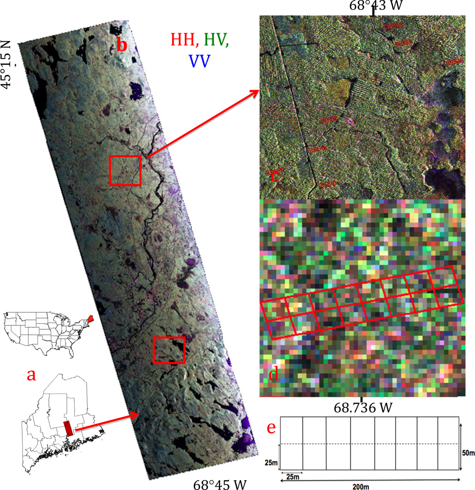
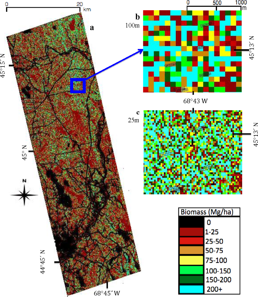
This research focuses on the temperate to boreal transitional forests in Howland (45.3°N, 68.8°W) and Penobscot (44.8°N, 68.6°W) Experimental Forests located in Maine (Figure 1). The forest is a mixed deciduous-coniferous forest and is a natural ecotone between a northern hardwood forest to the south and a boreal softwood forest to the north [12]. The dominant species are Eastern Hemlock (Tsuga canadensis), Red Spruce (Picea rubens), Balsam Fir (Abies balsamea), Paper Birch (Betula papyrifa), Red Maple (Acer rubrum) and several species of Aspen (Populus gradidentata, Populus tremuloides) (

Appendix 1. Ground estimates of Above Ground Biomass (AGB) and component AGB, developed with individual tree DBH and allometric equations.

Plot	Plot Area	AGB Density (Mg·ha−1)	Basal Area Density (m2·ha−1)	Crown AGB (Mg·ha−1)	Stem AGB (Mg/ha)	Old Growth or 2nd Forest
H02_2009	1 ha	27.39	5.81	7.25	20.13	SF
H03_2009	1 ha	38.86	8.80	9.72	25.75	SF
H05_2009	1 ha	109.65	22.43	27.40	82.25	OG
H06_2009	1 ha	62.46	12.80	16.52	45.95	SF
H07_2009	1 ha	216.48	44.76	60.16	156.32	OG
H08_2009	1 ha	17.40	4.65	4.39	13.01	SF
H09_2009	1 ha	123.59	24.28	30.43	91.56	OG
H10_2009	1 ha	235.35	46.07	57.19	178.16	OG
H12_2009	1 ha	178.43	38.26	44.56	133.88	OG
H17_2009	1 ha	147.74	27.92	36.95	110.79	OG
H18_2009	1 ha	136.12	26.20	34.78	101.34	OG
H04_2010	1 ha	131.63	26.82	33.42	98.21	OG
H07_2010	1 ha	145.57	25.58	37.28	108.29	OG
H08_2010	1 ha	124.78	25.01	34.39	90.26	OG
H20_2010	1 ha	114.54	25.44	30.95	83.59	OG
H21_2010	1 ha	113.46	26.99	29.39	84.06	OG
H22_2010	1 ha	174.27	24.86	45.05	129.22	OG
H23_2010	1 ha	114.72	22.87	28.65	86.08	OG
HT1_2010	1 ha	203.22	22.48	51.18	152.20	OG
HT2_2010	1 ha	191.72	24.10	46.58	145.15	OG
P01_2009	1 ha	257.19	46.21	61.83	195.36	OG
P03_2009	1 ha	137.31	37.18	38.90	98.41	OG
P04_2009	1 ha	49.26	12.35	15.82	33.44	SF
P05_2009	1 ha	147.43	27.41	34.48	112.95	OG
P06_2009	1 ha	60.50	13.76	16.60	43.90	SF
P07_2009	1 ha	141.39	26.47	33.23	108.17	OG
P09_2009	1 ha	1.70	7.71	0.76	0.94	SF
P10_2009	1 ha	138.98	26.17	35.10	103.88	OG
P11_2009	1 ha	108.81	21.13	24.30	72.59	OG
P13_2009	1 ha	201.87	34.08	54.66	147.21	OG
P14_2009	1 ha	22.21	4.42	6.97	15.24	SF
P15_2009	1 ha	226.5	41.43	57.68	168.82	OG

). The forests are generally fragmented due to both natural disturbance and logging or management practices [13,30]. Due to a long history of forest use, the study area is covered by a range of unmanaged old-growth forest stands, regeneration of varied ages, and small tree plantations [13,30]. Soil drainage classes and soil types can be highly variable within a small area due to a history of glaciation [12]. The variability of soil types limits the occurrence of single species stands, and coupled with varied histories of land-use has resulted heterogeneity of tree species and forest communities. Because of this, aboveground biomass can differ significantly across space, from saturated bogs with low tree biomass to high biomass old growth stands [12].

2.2. Field Data Collection

To capture the landscape variability of the forest aboveground biomass, we established 32 1.0 ha plots in both private and public land in forests of varying age and degree of disturbance during the summer of 2009 and 2010. All 1.0 ha plots were 50 m × 200 m and aligned along the range direction of radar images and subdivided into 16 quadrants of 25 m × 25 m (0.0625 ha). We measured the location of all plots and subplots with GPS units (Garmin GPSMAP 60CSx) with approximately 5 m accuracy in the field providing twenty-seven geographical markers per hectare.

The plot orientation was established to be perpendicular to the known flight direction of the UAVSAR mission, with the 200 m side aligned with the range direction of the UAVSAR flight lines, so as to encompass as much information as possible across changing local incidence angles and reduce the effects of pixel location and tree shadowing in radar backscatter extraction (Figure 1).

We measured all trees above 10 cm in diameter at breast height (DBH), identified the tree species, and mapped them within each plot. The aboveground biomass for individual trees was estimated using previously defined genus-specific equations [31]. These equations have been used in Forest Inventory and Analysis estimates of the US forest carbon storage [32]. However, while the Forest Inventory and Analysis plot data is small (0.4 ha) and may not be very suitable for remote sensing analysis, their methods of aboveground biomass estimation are applicable to our field data. The aboveground biomass was determined for individual trees based on whether they were hardwood or softwood species (Mg), summed to get total AGB per plot size (Mg/area), then divided by the plot area to determine AGB normalized to a hectare (Mg·ha⁻¹). We used the combination of subplot data to estimate aboveground biomass at different spatial scales of 0.0625 ha, 0.25 ha, 0.5 ha, and 1.0 ha. We also estimated the biomass of tree components, such as foliage, branch, and stem using the Jenkins equations based on hardwood and softwood tree species and reported the total aboveground biomass, basal area, crown aboveground biomass, and stem aboveground biomass for all 1.0 ha plots (Appendix 1). Aboveground biomass results from these equations, regardless of any potential errors, were assumed to be the estimate of the true aboveground biomass of the forest [3,31,32].

2.3. Remote Sensing Data

We use remote sensing data collected by NASA’s Unmanned Aerial Vehicle Synthetic Aperture Radar (UAVSAR) in August 2009. UAVSAR is an airborne polarimetric L-band radar sensor, which was designed for repeat-pass interferometry differential measurements in order to provide surface deformation measurements [33]. The UAVSAR flies at an altitude of 13,800 m and collects data in the L-band (24 cm wavelength) at 80 MHz bandwidth. The nominal resolution is 1.66 m in slant range and 0.6 m in azimuth. The multi-looked imagery is provided in geographic latitude and longitude coordinates (with WGS-84 geoid) at a pixel resolution of 0.00005556 degrees, or approximately 5 m × 5 m. The backscatter was collected and is reported here in power units (m²/m²), instead of the typically reported db units, although it is just a logarithmic conversion between the two. Data was collected over the study area on four different dates (5, 6, 7, and 14 August 2009). Based on temporal variation (See Section 4.3), all analysis was done on three images from 5 August 2009 and one from 6 August. Before our access to the images, the UAVSAR images were initially corrected for any potential terrain effects and ground-projected despite relatively small topographical variations across the study area (less than 20 m) [33]. UAVSAR was flown repeatedly over the study area by shifting the flight lines along the same headings to change the incidence angle in the middle of the swath by 10° increments in either direction and to image the field plots at incidence angles from 20 to 70 degrees. We refer to these flight lines as FL1, FL2, FL3, and FL4, respectively representing a range of low to high incidence angles (20°, 30°, 40°, 50°), respectively.

2.4. Impact of Radar Incidence Angle

We used four different images from which the extracted backscatter values were used to analyze the effect of the incidence angles. The incidence angle of the radar signal as it interacts with the surface has a direct effect on the resultant backscatter, and thus needs to be either corrected or introduced implicitly in the algorithm in order to accurately estimate biomass for all the pixels within the image.

From an incidence angle image across the whole swath, the local incidence angles of each plot were derived from the pixels within the plot (

Appendix 3. Individual plot incidence angles, in degrees, for each incidence angle image. Converted to radians for backscatter correction.

Plot	FL1	FL2	FL3	FL4
P01_09	39.87	46.42	50.98	65.68
P03_09	40.04	46.55	50.86	65.73
P04_09	38.97	45.69	51.57	65.42
P05_09	39.49	46.10	51.24	65.57
P06_09	42.20	48.29	49.31	66.35
P07_09	40.52	46.94	50.54	65.86
P09_09	39.47	46.09	51.26	65.56
P10_09	37.33	44.36	52.58	64.95
P11_09	36.85	43.97	52.86	64.82
P13_09	34.59	42.14	54.08	64.18
P14_09	33.85	41.57	54.26	63.98
P15_09	43.36	49.23	48.36	66.69
H02_09	36.73	43.90	52.72	64.79
H03_09	36.53	43.74	52.83	64.73
H05_09	34.70	42.26	53.82	64.22
H06_09	39.79	46.37	50.82	65.66
H07_09	32.64	40.58	54.84	63.64
H08_09	33.82	41.54	54.27	63.97
H09_09	40.34	46.81	50.45	65.81
H10_09	41.86	48.04	49.34	66.26
H12_09	41.69	47.90	49.47	66.21
H17_09	43.67	49.49	47.91	66.79
H18_09	40.66	47.07	50.26	65.91
H04_2010	23.37	32.94	58.45	61.08
H07_2010	24.34	33.75	58.14	61.35
H08_2010	25.10	34.38	57.88	61.56
H20_2010	23.91	33.40	58.24	61.23
H21_2010	22.67	32.36	58.64	60.89
H22_2010	24.01	33.48	58.24	61.26
H23_2010	22.91	32.55	58.60	60.95
HT1_2010	41.76	47.96	49.41	66.23
HT2_2010	40.41	46.87	50.40	65.83

). In order to correct, the center of the swath’s incidence angle was needed, and was determined to be 52.7°. The extracted backscatter values were corrected at the plot level utilizing the individual plot incidence angles across four images and using the following normalizing relation:

$${\sigma }_{\mathit{corr}}^0={\sigma }_{\mathit{raw}}^0{\left(\frac{\mathit{cos}\theta }{\mathit{cos}{\theta }_0}\right)}^n$$

(1)

θ₀ is the average incidence angle at the center of the UAVSAR image swath and is approximately 52.7°, the power n is approximately 1.4 and is estimated by fitting the above model to the incidence angle of the backscatter over all land cover types and image acquisitions [10]. The angle θ represents the local incidence angle at each pixel. The GPS coordinates collected at the center and side axes of each plot were converted to shapefiles and were then used to extract backscatter from the different UAVSAR images. The backscatter extraction was performed at all four spatial scales (0.0625 ha, 0.25 ha, 0.5 ha, and 1.0 ha), and on all dates. All backscatter values from four incidence angle images taken on 5 August 2009 were compiled together and corrected in one dataset, using the above equation and then aggregated in two manners to compare to the ground data. First, the data was compiled into an extensive list with backscatter values from each individual incidence angle image, with three or four backscatter values for each plot AGB value. Secondly, the multiple backscatter values from the different images were averaged, so there was only one value per plot. This resulted in two different estimation algorithms for each spatial resolution to predict the square root of aboveground biomass.

2.5. Spatial Analysis

We developed parametric models based on regression models between backscatter at different polarizations and aboveground biomass. Although regression models do not provide detailed information about variables that impact the radar backscatter, they appear to be realistic in terms of demonstrating the impact of radar configuration such as incidence angles or environmental variables on radar sensitivity to aboveground biomass [2,13,16,29,34]. The models were developed at different spatial scales by extracting the backscatter values over the 1.0 ha plots. We had 32 1.0 ha ground plots, with sixteen 25 m by 25 m subplots within each hectare, with a total of 512 subplots of 0.0625-ha. The analysis began with the smallest segment of ground data at 25 m by 25 m subplots, and then scaled up to 50 m × 50 m (0.25 ha), 50 m × 100 m (0.5 ha), and last 50 m × 200 m (1.0 ha). The impact of spatial scale on the variability of field-estimated aboveground biomass was assessed before relating it to radar backscatter. A calculation of the coefficient of variation (CV) was done for each plot size, by dividing the standard deviation by the mean, and multiplying by 100 to get a percentage.

2.6. Radar Estimation of Aboveground Biomass

We used a multivariate regression approach to examine the relationship between forest aboveground biomass and polarimetric backscatter from different acquisition dates. It was determined that the best relationship with AGB was with the data acquired on 5 August, so the remainder of the analysis focused on flight lines FL1, FL2, and FL3 from 5 August, and FL4 from 6 August 2009 collections. By comparing the extracted backscatter with the ground estimated AGB values, we sought to determine the best spatial scale to assess biomass of this forest type solely through remotely sensed data.

Since the relationship between backscatter and aboveground biomass levels off at a certain value depending on frequency and incidence angle [2,16], the models were developed with the square root of aboveground biomass to develop the backscatter (in power units (m²/m²)) and aboveground biomass estimation algorithm [3]. By using R statistical software, linear regression models were developed at various scales with the three radar polarizations (HH, HV, VV) in the following form:

$$\sqrt{AGB}=a_0+a_1{\sigma }_{HH}^0+a_2{\sigma }_{HV}^0+a_3{\sigma }_W^0$$

(2)

The unknown coefficients (a₀, a₁, a₂, a₃) at four spatial scales are provided in

Table 1. Derived algorithm coefficients at each spatial scale and respective statistical values. The resultant values for predicted square root of AGB were then squared and compared to the ground AGB to determine R², P value, bias, and RMSE.

UAVSAR Averages	A0	A1	A2	A3	R2	P Value	Bias	Overall RMSE	RMSE <150 AGB
1	−4.15	3.16	246.16	−9.9	0.671	1.54e-07	−3.6	44.03	23.05
0.5	−0.93	−7.30	271.59	−24.7	0.607	8.00e-13	−4.7	47.57	30.72
0.25	−0.03	−13.48	279.35	−25.3	0.534	<2.2e-16	−6.3	53.54	39.88
0.0625	−0.56	2.91	232.38	−18.5	0.451	<2.2e-16	−7.5	62.24	45.29
UAVSAR Compiled
1	0.62	−13.50	276.36	−18.3	0.500	<2.2e-16	−5.9	49.20	34.90
0.5	1.48	−24.82	280.28	−17.1	0.482	<2.2e-16	−5.8	53.06	40.27
0.25	4.48	−18.28	193.35	−4.2	0.291	<2.2e-16	−7.1	58.10	45.80
0.0625	5.99	−2.40	111.94	−6.2	0.187	<2.2e-16	−10.4	69.02	50.17

In form: √(AGB) = a₀ + a₁σ_HH + a₂σ_HV + a₃σ_VV.

. By combining the three different polarizations, we aimed to include different forest structural information represented in scattering mechanisms by polarimetric measurements in the algorithm [35]. Once the equations were developed, we determined RMSE of the entire dataset, as well as for the plots with initial AGB < 150 Mg·ha⁻¹, where the sensitivity decreases. We reported the error estimation of both the compiled and averaged models at each spatial resolution to understand the accuracy and capabilities of SAR estimation of aboveground biomass.

3. Results

3.1. Variability of Stem Number and Plot Aboveground Biomass

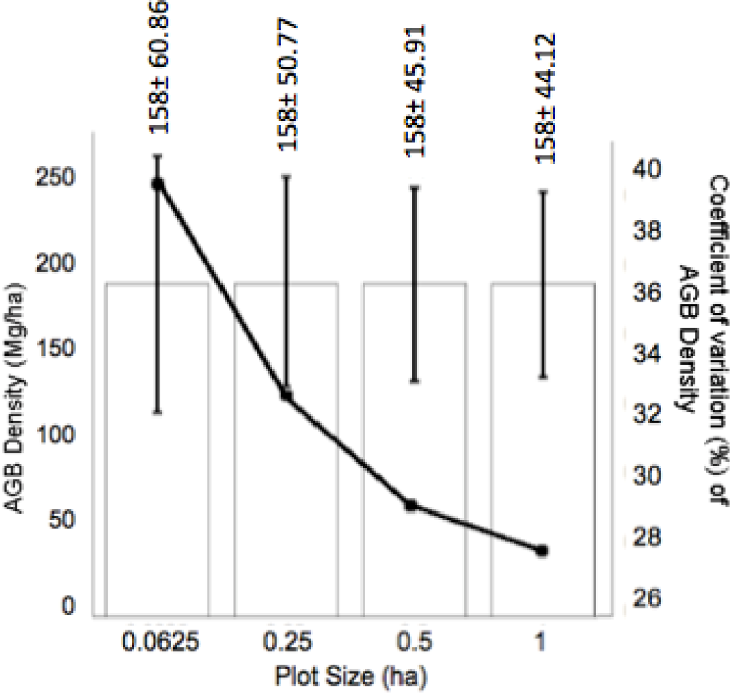
We first assessed the variability of AGB within each plot and across spatial scales. We identified 24,906 stems ≥ 10 cm DBH from a total of 39 tree species from 32 1.0 ha plots, with an average of 778 individuals per plot, and a range from 58 to 2,253 individuals per hectare. At all spatial scales, the average aboveground biomass was 158.1 Mg·ha⁻¹, while the coefficient of variation decreased with increasing plot size (Figure 2).

As plot size increased, standard deviation decreased, from 60.9 Mg·ha⁻¹ at the 0.0625 ha scale to 44.1 Mg·ha⁻¹ at the 1.0 ha scale. In addition the coefficient of variation drops significantly from 0.38 to 0.27 from the smallest scale to the largest scale. This shows that the initial variability of our field data increases as plot size decreases. At smaller scales (0.0625 ha), subplots may be disturbed and in a state of regeneration with low AGB, while being adjacent to a high AGB subplot. At larger scales, these differences become averaged out and less severe, resulting in a lower coefficient of variation across the plots at the 1.0 ha scale.

3.2. Incidence Angle Effect

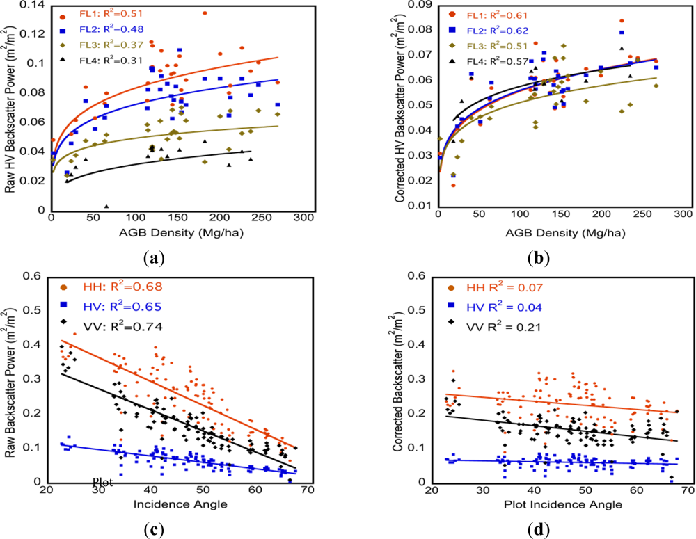
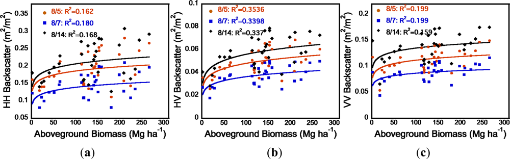
The raw extracted backscatter values from each UAVSAR image were compared with aboveground biomass. As incidence angle increased, the correlation between field plot estimated aboveground biomass and radar backscatter decreased Figure 3(a). The relationship for the HV polarization resulted in R² values of 0.51, 0.48, 0.37, and 0.31 from low to high incidence angles along the flight line (Figure 3(a)). After applying the correction to the backscatter values, the R² values all increased, to 0.61, 0.62, 0.51, 0.57, respectively (Figure 3(b)). In addition, the regression curves lie much more closely together, meaning that the relationship between the field aboveground biomass and the different backscatter values across incidence angles for each plot are more similar.

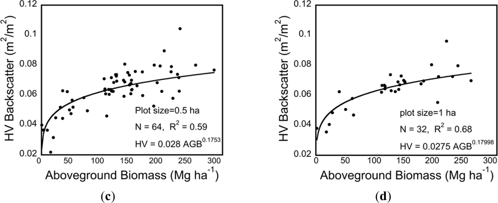
3.3. Radar Backscatter Sensitivity to Biomass

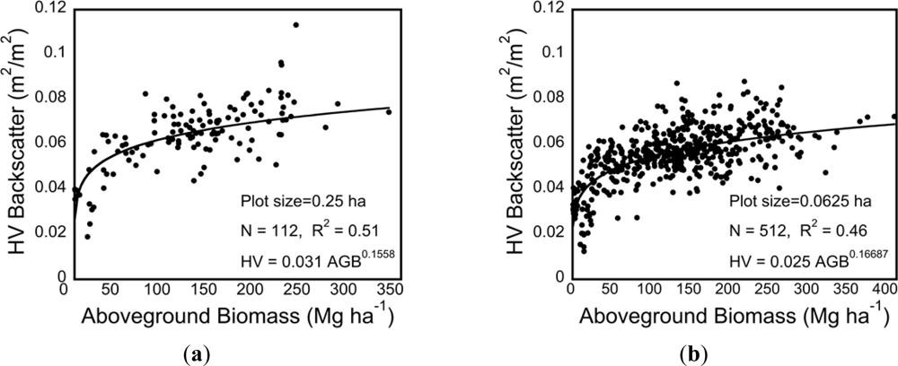
The relationship of aboveground biomass to the uncorrected UAVSAR backscatter shows that lower incidence angles have higher backscatter values than the same plot at a higher incidence angle, as well as higher R² values (Figure 3(a)). After the reduction of the effect of incidence angle on the radar backscatter values, all polarizations were compared to the field plots at the four spatial scales. For all polarizations (HH, HV, and VV), the R² of this relationship increased as plot size increased, with the most dispersion at 0.0625 ha and the least variability at 1.0 ha. This relationship for the corrected HV backscatter had the highest R² of the three polarizations at all spatial scales (0.46, 0.51, 0.59, and 0.68) as plot size increased (Figure 4).

For HH, the R² values for increasing spatial scale were 0.28, 0.39, 0.49, 0.58, while for the VV polarization, they were 0.11, 0.31, 0.38, and 0.46. The cross-polarized HV has the highest correlation to field aboveground biomass, followed by HH, then VV for all spatial scales. Because of these differences between polarizations, all three were combined into a single algorithm for each spatial scale in order to emphasize the benefits of each.

3.4. Impact of Spatial Scales on Radar Estimation of Biomass

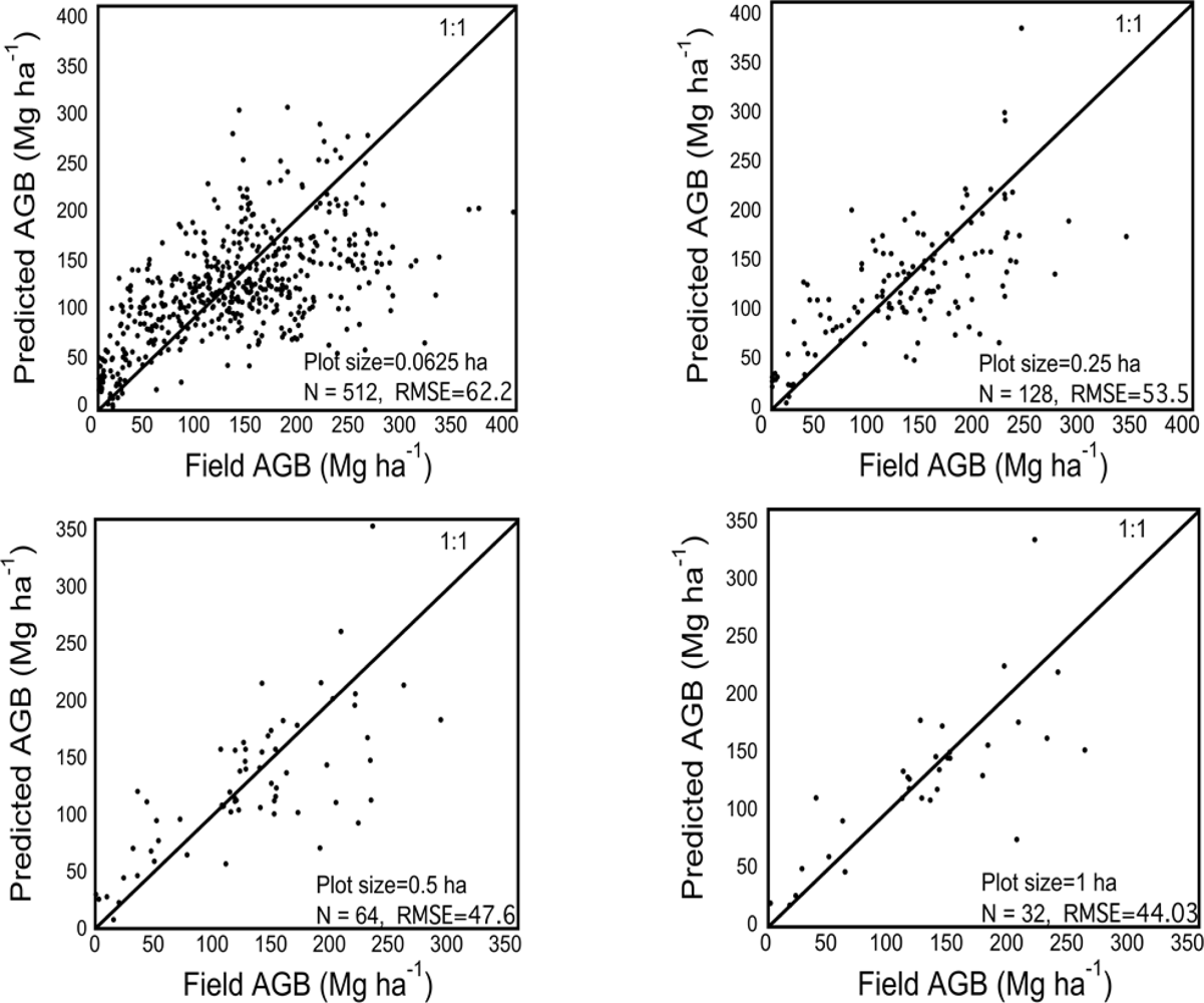
Several different linear regression models were developed comparing the square root of aboveground biomass to corrected backscatter values. These predictive algorithms were determined for four different spatial scales: 0.0625 ha, 0.25 ha, 0.5 ha, and 1.0 ha and for the full compiled dataset and the averaged dataset. The results were compared to our field AGB density for each plot. A graph comparing field AGB density to our predicted AGB density would ideally have a 1:1 relationship. For both the full compiled and the averaged values that were used to make the predictions, the RMSE values increased with decreasing plot size. The model results for the averaged data only can be seen in Figure 6. Overall, the average backscatter analysis resulted in higher R² values and lower RMSE than the compiled data. The model with the best relationship was the model using the average backscatter across images at the 1.0 ha spatial scale, with an R² of 0.67, p value of 1.54e-7, and an overall RMSE of 44 Mg·ha⁻¹ (Figure 5, Table 1).

RMSE was calculated for both the compiled and averaged datasets, reported in Table 1. For both sets of analyses, the RMSE values decreased with increasing plot size, meaning that there are more errors associated with smaller plot size (Table 1). RMSE was lower for the averaged data, which resulted in the best model. Due to the loss of sensitivity of SAR data at high levels of AGB, RMSE was also assessed for just the plots with 150 Mg·ha⁻¹ or less of AGB. For this case, at 1 ha using averaged backscatter values, RMSE dropped to 23.05 Mg·ha⁻¹, from 44.03 Mg·ha⁻¹ on the entire dataset. Similarly, at the 0.0625 ha scale, RMSE dropped to 45.29 Mg·ha⁻¹ from 62.24 when looking at just plots less than 150 Mg·ha⁻¹. Bias was calculated on the residuals for both the compiled data and the averaged values. In both cases, the predicted aboveground biomass underestimates the measured aboveground biomass at all spatial scales, ranging from −3.6 (1 ha) to −7.5 (0.0625 ha) for the averaged backscatter values. The underestimation is slightly more for the compiled dataset than the averaged dataset, but not significantly so.

3.5. Mapping Landscape Aboveground Biomass

The resulting best models from the average backscatter values relating multiple radar polarizations to aboveground biomass were used to create AGB maps at 25 m and a 100 m pixel resolution (Figure 6). The images were resampled to these resolutions to match the scales used to create the regression equations. At the 100 m resolution, there were less than three pixels with any portion within the 1.0 ha plots, while at the 25 m scale, there are up to 20 pixels encompassed partially within the plot.

4. Discussion

4.1. Impact of Radar Resolution for Estimating AGB

The coefficient of variation drops significantly from 0.38 to 0.27 from the smallest plot size to the largest plot aggregation based solely on the field data, suggesting that the initial variability of forest structure in the plot data increases as plot size decreases, which in turn has an impact on estimation approach. The results also show that for all models there is a power relationship between aboveground biomass and backscatter values up to biomass values about 150 Mg·ha⁻¹, which is especially pronounced in the smaller plot size analyses. The sensitivity of the L-band radar to AGB declines drastically above this value indicating large errors with a significant underestimation (negative bias) at high values of aboveground biomass, especially at smaller scales. The RMSE reflects this, especially when analyzing the strength of the model only on the plots with less than 150 Mg·ha⁻¹ field aboveground biomass (Table 1). When assessing the maps of aboveground biomass, we can see that there are more high biomass pixels (>200 Mg·ha⁻¹) in the 25 m pixel size than the 100 m pixel size (Figure 6(b,c)). However, these low values are reduced when scaled up to 100 m pixel size. At smaller scales (0.0625 ha), there is more heterogeneity in forest structure and AGB with areas of natural disturbance and recovery along with forest thinning occurring at small scales. At larger scales, these differences become averaged out and less severe, resulting in a fewer pixels with higher biomass.

The results also showed larger bias in aboveground biomass estimation from radar at smaller scales, making the aggregation from small to larger scales an error-prone process, and suggesting significantly improved biomass estimation directly at scales of 1.0 ha. This also suggests that the Forest Inventory and Analysis plot data at 0.4 ha may not suitable for remote analyses of forest aboveground biomass [28]. The future analyses of aboveground biomass utilizing similar radar sensors may be most accurate at the 1.0 ha spatial scale and field data at smaller plot sizes may introduce too much variation or error into aboveground biomass estimates. We expect that the sensitivity to AGB may improve at large spatial sales when effects of forest structure and minor geolocation errors are averaged out. However, the maximum plot size available for this study does not allow us to test the above hypothesis.

4.2. Role of Polarization and Incidence Angle in Estimating AGB

Our results support past studies that the cross-polarized HV has the best correlation to forest aboveground biomass [2,19,20]. The importance of the HV backscatter value in the regression model is clear in the coefficients that are heavily weighted towards the HV value. To make our models more accurate, we combined three polarizations into one multivariate regression to estimate aboveground biomass, although the results of the model highly relied towards the HV value.

Having multiple incidence angles may allow for more information to be gleaned from the radar backscatter of forest but results in complications if corrections are not applied. Our correction for incidence angle made the backscatter have a stronger relationship to field estimated AGB for each image, as well as making it possible for the averaging across images, effectively making our assessment more robust. In general, radar backscatter observations at different incidence angles impact the inherent scattering mechanisms controlling the backscatter values at different polarization. Observations at closer to nadir incidence angles (20°–30°) will allow better penetration into the forest canopy and potentially larger sensitivity to AGB. However, at these incidence angles, radar backscatter becomes more sensitive to the underlying soil moisture variations and hence prone to larger AGB estimation errors. At steeper incidence angles (50°–60°), the scattering effects on the radar measurements are almost the opposite, suggesting lower sensitivity to AGB. For temperate forest of this type, data collected at 30°–40° incidence angles appear to be the most suitable for estimating AGB from L-band radar. Other biomes with varying canopy closure may be more sensitive to a different angle range.

4.3. Impact of Environmental Factors

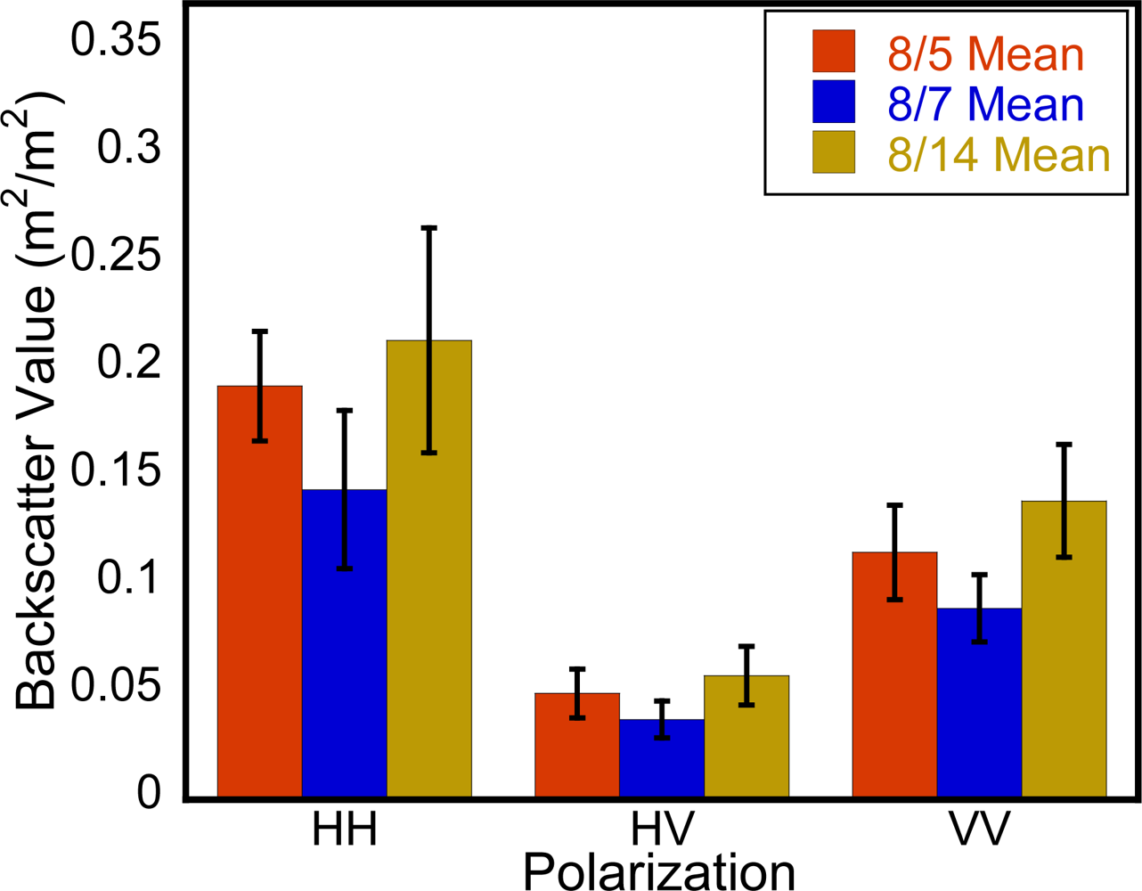
Differing levels of soil moisture can affect radar signals, particularly in areas with low biomass densities. In these areas, radar can penetrate through the trees and hit the surface, which is when soil moisture can affect backscatter [24]. Ranson et al.[13] previously determined that drainage characteristics vary widely in the study area, and since soil moisture information was not collected concurrently in our plot sites it could be a confounding factor in the AGB estimation. Comparing UAVSAR backscatter data collected on 5, 7 and 14 August 2009, we found distinct differences in values between days (Figure 7). See Appendix 5 for plot of each date’s backscatter compared to AGB, which shows clear differences between the curves.

These short-term variations in the data collection could be due to a variety of factors including effects of rain, impacting soil moisture, and wind, impacting orientation of leaves, as well as error in the initial data calibration [14]. Since vegetation and soil moisture have an impact on backscatter values, precipitation events could have caused the differences between the UAVSAR images on 5, 7, and 14 August 2009. The images are still useful and possible for analysis but since moisture parameters can change backscatter values, the developed algorithms are site and environmental condition specific. Our analysis used three flight lines from 5 August, and one from 6 August (50° incidence angle). The relationship derived from 5 August performed well across polarizations, and was between the lowest values from 7 August and the highest values from 14 August. Radar flights should be planned during the driest season to reduce temporal fluctuations in backscatter due to moisture.

4.4. Other Sources of Errors

Although this analysis found reasonable correlations between radar backscatter measurements and aboveground biomass, and resulted in predictive equations of aboveground biomass at the 1.0 ha scale with an R² of 0.67, there are several sources of errors to our estimation of AGB from radar imagery that are not accounted for in our analysis. The most dominant sources of errors include the errors associated with the use of allometric equations in inventory data and the accuracy of plot geolocation.

Allometric Estimating

The aboveground biomass assumed to be accurate, though in actuality is only an estimate of true tree biomass based on previously derived allometry developed by Jenkins [27], since to get the true aboveground biomass would require destructive sampling. Since this would destroy the forest stocks, estimating based on genus level relationships are the best method of quantifying biomass available for this species assemblage. Another shortcoming in the ground collected biomass values is that measurements were limited to trees ≥10 cm DBH, while smaller trees, and coarse woody debris and perhaps dead trees are also important pools of aboveground forest biomass that were left out of this assessment and may impact the radar backscatter [2].

Geolocation

Errors associated with the geo-referencing of plot corners and the relative location of these points with respect to the radar resolution can introduce large errors in radar backscatter analysis. These errors are likely to be more pronounced at the smaller subplot level than on the whole hectare. The AGB maps created over central Maine show the differences in analysis using different spatial resolution of the underlying image. When the pixels are 100 m × 100 m, there are only a few pixels that are encompassed by the plot borders that are averaged for the 1.0 ha (Figure 7(b)), while at the 25 m × 25 m resolution, there is much more variation present in the data (Figure 7(c)). If the entire hectare plot is geo-located with 5–10 m error, there is likely to be little difference of the overall plot structure. However, at the 25 m × 25 m level, 5–10 m off could entirely change the forest structure within the subplot, and thus the aboveground biomass density. Geo-referencing errors, both in the field and within the image processing and projection, likely affect the subplot biomass accuracy to a greater extent than at a larger scale. It is important to note that for all of the analyses, the R² value was found to be higher for the hectare plots, where there is less potential for geo-referencing errors to affect the data. The differences in spatial resolution of the two aboveground biomass maps show how pixel size of the remote sensing data could affect the analysis, had they not been averaged at each spatial scale from the initial high-resolution data.

5. Conclusions

The objective of this research was to determine a method for estimating aboveground biomass over temperate mixed forest landscapes in the Maine using the data from a SAR sensor that can be deployed on unmanned vehicles in the future to increase temporal and spatial resolution of forest aboveground biomass. Ground measurements over 32 ha plots with 512 25 m × 25 m subplots in 2009 and 2010 were used to calculate aboveground biomass values to determine relationships with data collected from the backscatter of the active UAVSAR sensor. This research developed useful regression equations to relate L-band radar to forest aboveground biomass density in the transitional mixed forest of Maine. Through this technique, the feasibility and scale of a L-band airborne radar sensor to estimate aboveground biomass was assessed. It was determined that the highest accuracy in estimation is at the 1.0 ha spatial scale, likely as errors due to heterogeneity are reduced when averaged over the larger scale.

Algorithms were developed that combined three radar backscatter polarizations (HH, HV, and VV) to estimate aboveground biomass at the four spatial scales. Among polarizations, the cross-polarized HV had the highest sensitivity to field estimated aboveground biomass. The predicted aboveground biomass from these algorithms resulted in decreasing estimation error as the pixel size increased. The model with the best relationship was the model using the average backscatter across images at the 1.0 ha spatial scale, with an R² of 0.67, p value of 1.54e-7, and an overall RMSE of 44 Mg·ha⁻¹ (Figure 5, Table 1). Due to the loss of sensitivity of SAR data at high levels of AGB, RMSE was also assessed for just the plots with 150 Mg·ha⁻¹ or less of AGB. For this case, at 1 ha using averaged backscatter values, RMSE dropped to 23 Mg·ha⁻¹, from 44 Mg·ha⁻¹ on the entire dataset. Similarly, at the 0.0625 ha scale, RMSE dropped to 45.29 Mg·ha⁻¹ from 62.24 when looking at just plots less than 150 Mg·ha⁻¹. Bias was calculated on the residuals for both the compiled data and the averaged values. In both cases, the predicted aboveground biomass underestimates the measured aboveground biomass at all spatial scales, ranging from −3.6 (1 ha) to −7.5 (0.0625 ha) for the averaged backscatter values. This study helped to determine algorithms that aided in modeling aboveground biomass for central Maine using L-band radar and resulted in the production of maps of aboveground biomass for the landscape.

Because our findings indicate highest accuracy of biomass retrieval with larger spatial resolution, it may not be necessary to rely on airborne collections of radar data with limited spatial coverage. With a spaceborne radar platform, data could be collected at a lower spatial resolution across larger geographic areas for global mapping. However, high-resolution datasets are immensely important to determine small-scale forest heterogeneity and the end goal of the research should dictate the platform used.

References

- Asner, G.P.; Hughes, R.F.; Mascaro, J.; Uowolo, A.L.; Knapp, D.E.; Jacobson, J.; Kennedy-Bowdoin, T.; Clark, J.K. High-resolution carbon mapping on the million-hectare island of Hawaii. Front. Ecol. Environ 2011, 9, 434–439. [Google Scholar]
- Le Toan, T.; Quegan, S.; Woodward, I.; Lomas, M.; Delbart, N.; Picard, G. Relating radar remote sensing of biomass to modelling of forest carbon budgets. Climatic Change 2004, 67, 379–402. [Google Scholar]
- Saatchi, S.; Marlier, M.; Chazdon, R.L.; Clark, D.B.; Russell, A.E. Impact of spatial variability of tropical forest structure on radar estimation of aboveground biomass. Remote Sens. Environ 2011, 115, 2836–2849. [Google Scholar]
- Houghton, R.A. Revised estimates of the annual net flux of carbon to the atmosphere from changes in land use and land management 1850–2000. Tellus B 2003, 55, 2836–2849. [Google Scholar]
- Kasischke, E.S.; Bourgeauchavez, L.L.; French, N.H.F. Observations of variations in ers-1 sar image intensity associated with forest-fires in alaska. IEEE Trans. Geosci. Remote Sens 1994, 32, 206–210. [Google Scholar]
- Sandberg, G.; Ulander, L.M.H.; Fransson, J.E.S.; Holmgren, J.; Le Toan, T. L- and P-band backscatter intensity for biomass retrieval in hemiboreal forest. Remote Sens. Environ 2011, 115, 2874–2886. [Google Scholar]
- Wigneron, J.-P.; Calvet, J.-C.; Guyon, D.; Courrier, G.; Grojean, O. Estimation of Coniferous Forest Characteristics from Passive Microwave Measurements. Proceedings of International Geoscience and Remote Sensing Symposium, Florence, Italy, 10–14 July 1995; 1, pp. 725–727.
- Kurvonen, L.; Pulliainen, J.; Hallikainen, M. Active and passive microwave remote sensing of boreal forests. Acta Astronaut 2002, 51, 707–713. [Google Scholar]
- Pulliainen, J.T.; Kurvonen, L.; Hallikainen, M.T. Multitemporal behavior of l- and c-band sar observations of boreal forests. IEEE Trans. Geosci. Remote Sens 1999, 37, 927–937. [Google Scholar]
- Ahmed, R.; Siqueira, P.; Bergen, K.; Chapman, B.; Hensley, S. A Biomass Estimate over the Harvard Forest Using Field Measurements with Radar and Lidar Data. Proceedings of 2010 IEEE International Geoscience and Remote Sensing Symposium (IGARSS), Honolulu, HI, USA, 25–30 July 2010.
- Hensley, S.; Chapman, B.; Neumann, M.; Lavalle, M.; Michel, T.; Oveisgharan, S.; Muellerschoen, R.; Siqueira, P.; Ahmed, R. Polarimetric Interferometric Studies of the Harvard Forest Using L-Band UAVSAR Data Repeat Pass Data. Proceedings of 2011 3rd International Asia-Pacific Conference Synthetic Aperture Radar (APSAR), Seoul, Korea, 26–30 September 2011; pp. 1–2.
- Ranson, K.J.; Sun, G.Q. Mapping biomass of a northern forest using multifrequency sar data. IEEE Trans. Geosci. Remote Sens 1994, 32, 388–396. [Google Scholar]
- Ranson, K.J.; Sun, G.; Weishampel, J.F.; Knox, R.G. Forest biomass from combined ecosystem and radar backscatter modeling. Remote Sens. Environ 1997, 59, 118–133. [Google Scholar]
- Simard, M.; Hensley, S.; Lavalle, M.; Dubayah, R.; Pinto, N.; Hofton, M. An empirical assessment of temporal decorrelation using the uninhabited aerial vehicle synthetic aperture radar over forested landscapes. Remote Sens 2012, 4, 975–986. [Google Scholar]
- Frelich, L. Forest Dynamics and Disturbance Regimes: Studies from Temperate Evergreen-Deciduous Forests; Cambridge University Press: Cambridge, UK, 2002. [Google Scholar]
- Saatchi, S.; Halligan, K.; Despain, D.G.; Crabtree, R.L. Estimation of forest fuel load from radar remote sensing. IEEE Trans. Geosci. Remote Sens 2007, 45, 1726–1740. [Google Scholar]
- Brown, S. Estimating Biomass and Biomass Change of Tropical Forests: A Primer; Food and Agriculture Organization of the United Nations: Rome, Italy, 1997. [Google Scholar]
- Elias, M.; Potvin, C. Assessing inter- and intra-specific variation in trunk carbon concentration for 32 neotropical tree species. Can. J. Forest Res 2003, 33, 1039–1045. [Google Scholar]
- Chave, J.; Andalo, C.; Brown, S.; Cairns, M.A.; Chambers, J.Q.; Eamus, D.; Folster, H.; Fromard, F.; Higuchi, N.; Kira, T.; et al. Tree allometry and improved estimation of carbon stocks and balance in tropical forests. Oecologia 2005, 145, 87–99. [Google Scholar]
- Gibbs, H.K.; Brown, S.; Niles, J.O.; Foley, J.A. Monitoring and estimating tropical forest carbon stocks: Making REDD a reality. Environ. Res. Lett 2007, 2, 045023. [Google Scholar]
- Zhang, N.; Yu, Z.L.; Yu, G.R.; Wu, J.G. Scaling up ecosystem productivity from patch to landscape: A case study of changbai mountain nature reserve, china. Landsc. Ecol 2007, 22, 303–315. [Google Scholar]
- Sun, G.; Ranson, K.J. Forest Biomass Retrieval from Lidar and Radar. Proceedings of 2009 IEEE International Geoscience and Remote Sensing Symposium (IGARSS), Cape Town, South Africa, 12–17 July 2009.
- Harrell, P.A.; Kasischke, E.S.; BourgeauChavez, L.L.; Haney, E.M.; Christensen, N.L. Evaluation of approaches to estimating aboveground biomass in southern pine forests using SIR-C data. Remote Sens. Environ 1997, 59, 223–233. [Google Scholar]
- Luckman, A.; Baker, J.; Kuplich, T.M.; Yanasse, C.D.F.; Frery, A.C. A study of the relationship between radar backscatter and regenerating tropical forest biomass for spaceborne SAR instruments. Remote Sens. Environ 1997, 60, 1–13. [Google Scholar]
- Kasischke, E.S.; Tanase, M.A.; Bourgeau-Chavez, L.L.; Borr, M. Soil moisture limitations on monitoring boreal forest regrowth using spaceborne L-band SAR data. Remote Sens. Environ 2011, 115, 227–232. [Google Scholar]
- Imhoff, M.L. A theoretical-analysis of the effect of forest structure on synthetic-aperture radar backscatter and the remote-sensing of biomass. IEEE Trans. Geosci. Remote Sens 1995, 33, 341–352. [Google Scholar]
- Richards, J.A.; Sun, G.Q.; Simonett, D.S. L-band radar backscatter modeling of forest stands. IEEE Trans. Geosci. Remote Sens 1987, 25, 487–498. [Google Scholar]
- Quegan, S.; Le Toan, T.; Yu, J.J.; Ribbes, F.; Floury, N. Multitemporal ERS SAR analysis applied to forest mapping. IEEE Trans. Geosci. Remote Sens 2000, 38, 741–753. [Google Scholar]
- Dobson, M.C.; Ulaby, F.T.; Letoan, T.; Beaudoin, A.; Kasischke, E.S.; Christensen, N. Dependence of radar backscatter on coniferous forest biomass. IEEE Trans. Geosci. Remote Sens 1992, 30, 412–415. [Google Scholar]
- Forest Ecosystem Research at Howland, Maine, Available online: http://howlandforest.org (accessed on 22 August 2009).
- Jenkins, J.C.; Chojnacky, D.C.; Heath, L.S.; Birdsey, R.A. National-scale biomass estimators for united states tree species. For. Sci 2003, 49, 12–35. [Google Scholar]
- Heath, L.; Hansen, M.; Smith, J.; Smith, B.; Miles, P. Investigation into Calculating Tree Biomass and Carbon in the FIADB Using a Biomass Expansion Factor Approach. Presented at the Forest Inventory and Analysis Symposium, Park City, UT, USA, 21–23 October 2008.
- NASA’s Jet Propulsion Laboratory. Uninhabited Aerial Vehicle Synthetic Aperture Radar. Available online: http://uavsar.jpl.nasa.gov (accessed on 1 March 2011).
- Saatchi, S.; Moghaddam, M. Estimation of Boreal Forest Biomass Using Spaceborne SAR Systems. Proceedings of IEEE 1999 International Geoscience and Remote Sensing Symposium (IGARSS ’99), Hamburg, Germany, 28 June 1999–2 July 1999.
- Saatchi, S.S.; McDonald, K.C. Coherent effects in microwave backscattering models for forest canopies. IEEE Trans. Geosci. Remote Sens 1997, 35, 1032–1044. [Google Scholar]