Article

Influence of Multi-Source and Multi-Temporal Remotely Sensed and Ancillary Data on the Accuracy of Random Forest Classification of Wetlands in Northern Minnesota

by
Jennifer M. Corcoran
1,*,
Joseph F. Knight
1 and
Alisa L. Gallant
2
1
Department of Forest Resources, University of Minnesota, 1530 Cleveland Ave. N, St. Paul, MN 55108, USA
2
Earth Resources Observation and Science Center, US Geological Survey, Sioux Falls, SD 57198, USA
*
Author to whom correspondence should be addressed.
Remote Sens. 2013, 5(7), 3212-3238; https://doi.org/10.3390/rs5073212
Submission received: 5 April 2013 / Revised: 20 June 2013 / Accepted: 20 June 2013 / Published: 4 July 2013

Abstract

:
Wetland mapping at the landscape scale using remotely sensed data requires both affordable data and an efficient accurate classification method. Random forest classification offers several advantages over traditional land cover classification techniques, including a bootstrapping technique to generate robust estimations of outliers in the training data, as well as the capability of measuring classification confidence. Though the random forest classifier can generate complex decision trees with a multitude of input data and still not run a high risk of over fitting, there is a great need to reduce computational and operational costs by including only key input data sets without sacrificing a significant level of accuracy. Our main questions for this study site in Northern Minnesota were: (1) how does classification accuracy and confidence of mapping wetlands compare using different remote sensing platforms and sets of input data; (2) what are the key input variables for accurate differentiation of upland, water, and wetlands, including wetland type; and (3) which datasets and seasonal imagery yield the best accuracy for wetland classification. Our results show the key input variables include terrain (elevation and curvature) and soils descriptors (hydric), along with an assortment of remotely sensed data collected in the spring (satellite visible, near infrared, and thermal bands; satellite normalized vegetation index and Tasseled Cap greenness and wetness; and horizontal-horizontal (HH) and horizontal-vertical (HV) polarization using L-band satellite radar). We undertook this exploratory analysis to inform decisions by natural resource managers charged with monitoring wetland ecosystems and to aid in designing a system for consistent operational mapping of wetlands across landscapes similar to those found in Northern Minnesota.

1. Introduction

Wetlands provide many ecosystem services such as filtering polluted water [1], mitigating flood damage [24], recharging groundwater storage [5,6], and providing habitat for diverse flora and fauna [79]. Wetland quality and quantity are particularly important in light of the increasing impacts of climate change, a growing human population, and changing land cover and land use practices [10,11]. It is therefore essential that wetlands are managed appropriately and monitored frequently.
The US Army Corps of Engineers defines wetlands as: “areas that are inundated or saturated by surface or ground water at a frequency and duration sufficient to support, and that under normal circumstances do support, a prevalence of vegetation typically adapted for life in saturated soil conditions” [12]. The Corps identifies potential wetland areas using three broad categories: soils, vegetation, and hydrology, where the classification is specifically based on geological substrate (soil type, drainage), the presence and type of hydrophytic vegetation, and topographic features that influence the hydrological movement and storage of water.
Characteristics of wetland structure and position are not the only influential factors on the permanence and duration of a wetland’s capacity to store water. Regional and local climate conditions are the main driving forces behind a wetland’s hydroperiod. Hydroperiod can be defined as the seasonal pattern of water level, duration and frequency in a wetland, akin to a “hydrologic signature”. The hydroperiod of a wetland has been described by Wissinger [13] as the single most important aspect of the biodiversity within a wetland habitat, because the duration between dry and wet periods directly influences complex biological interactions and communities. The phenology of a wetland has a major influence on its classification and changes in the hydroperiod over time can thus alter a wetland’s classification.
Accurate landscape-scale wetland maps are important for stakeholders that represent many different interests in wetland ecosystems. Accurate wetland maps are needed to: better respond to and prepare for natural disasters and invasive species mediation [14,15], conserve and restore wetland areas following policy and regulation changes [16,17], address water quality and quantity concerns [18,19], and better understand the linkages and seasonality of these ecosystems to biodiversity and other natural resources [20,21]. However, many existing wetland maps are out of date and efforts for updating them tend to happen over small geographic extents or at intervals too infrequent for appropriate environmental mitigation [22]. Furthermore, traditional wetland mapping methods often rely on optical imagery and manual photo interpretation or classification using single date imagery. These maps typically under-represent ephemeral and forested wetlands, due to their possible absence during time of data acquisition and because of obscuration by vegetative canopy [18]. Even if the temporal coverage is appropriate, optical imagery alone may not reveal wetlands obscured by clouds or haze, or a dense vegetated canopy.
The integration of multi-source (multi-platform and multi-frequency) and multi-temporal remotely sensed data can provide information for mapping wetlands in addition to the use of single date optical imagery traditionally used for wetland classification. Surface features, such as extent of inundation, vegetation structure, and likelihood of wetlands can be better resolved with the addition of longer wavelength radiometric responses, topographic derivatives [23], and ancillary data about the geological substrate [24,25]. Long-wave radar signals, such as C-band (5.6 cm) or L-band (23 cm), have been found to improve land cover classification accuracy because these wavelengths have deeper canopy penetration and are sensitive to soil moisture and inundation [2628]. These active sensors are not as sensitive to atmospheric effects, penetrate clouds, and are operational at night, thereby increasing the temporal coverage of wetland mapping. Research has shown that data from multiple sources and over multiple seasons capture greater variation in hydroperiod and vegetative condition and thus have the potential to increase both classification accuracy and confidence [2931].
Given the wealth of remotely sensed and ancillary data, a robust wetland classification method applied to large geographic areas needs to be computationally fast, require no assumptions about data distribution, handle nonlinearity in relations between input variables, and be capable of using numeric and categorical data. In addition, the assessment of results will be improved if the classification method identifies outliers in the training data, provides rankings of the importance of the input variables, and produces internal estimates of error and confidence of the output classification. Many decision tree classifiers fulfill all these requirements and have been used in land cover mapping for years [3235], including several that use the meta-classifier random forest [3638].
Our goal was to identify an optimal selection of input data from multiple sources and time periods of remotely sensed and ancillary data for accurate wetland mapping using random forest decision tree classification in a forested region of Northern Minnesota. We assessed ways of increasing classification accuracy, confidence, and practicality by assessing results from several combinations of input data. Our main questions for this study site in Northern Minnesota were: (1) how does classification accuracy and confidence of wetland mapping compare using different remote sensing platforms and ancillary data from different periods of the growing season; (2) what are the key input variables for accurate differentiation of upland, water, and wetlands, including wetland type; and (3) which datasets and seasonal imagery yield the best accuracy for wetland classification.

2. Methods

2.1. Study Area

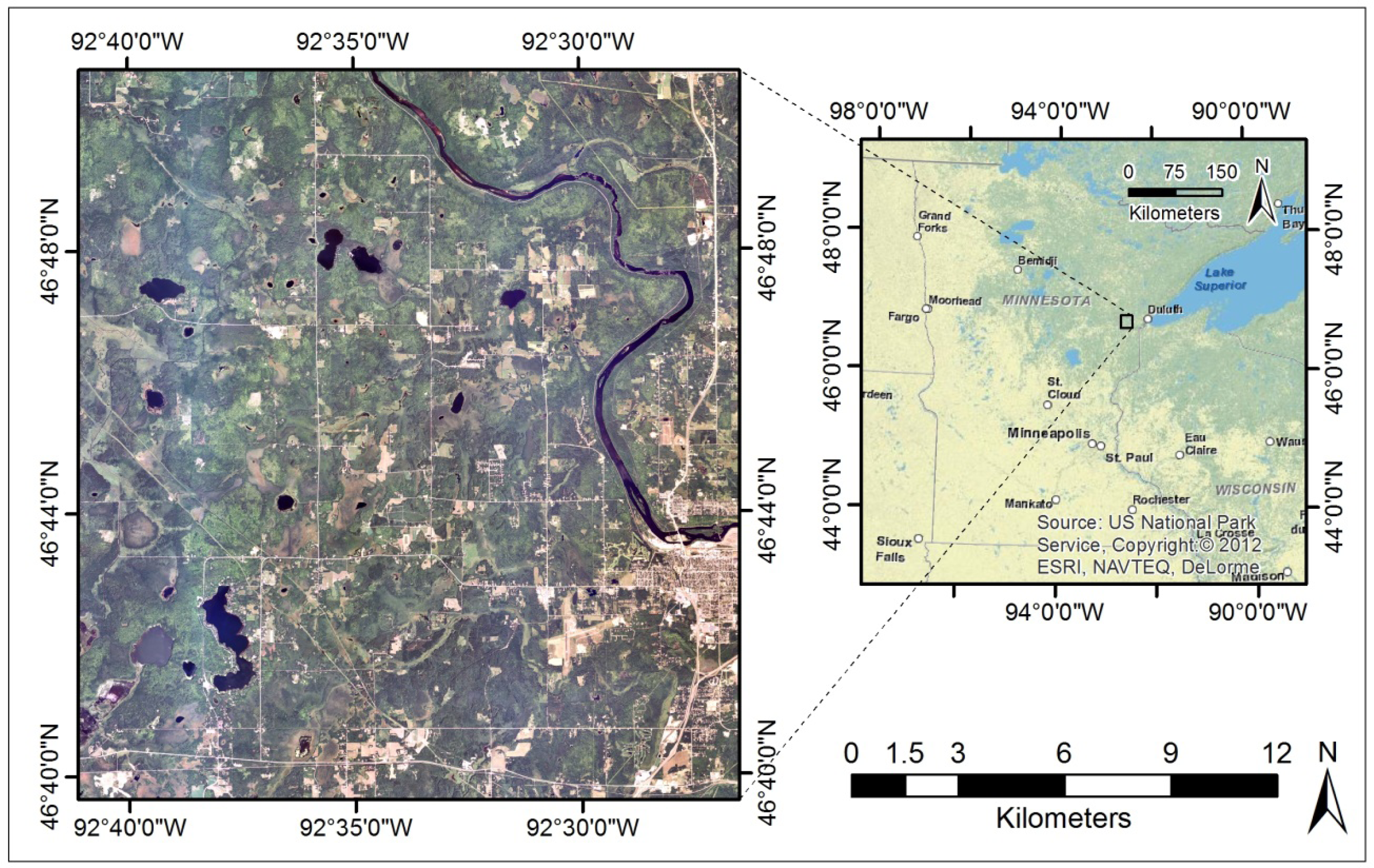
Much of northern Minnesota (MN) is forested. The hydrographic patterns of the landscape have been influenced heavily by glacial advances and retreats over the millennia [39]. Our study centered on Cloquet, MN (Figure 1), which lies in the sparsely populated “Arrowhead” region of northeastern Minnesota. This study area is dominated by managed and natural hardwood and conifer forests, woody and herbaceous wetlands [40], and low density residential housing with a small city center (population 12,000) [41]. The elevation across the study area is 330–450 m above sea level (mean of 392 m), with the slope of the landscape averaging less than 1.7 degrees.
Given the variable nature of hydroperiod in space and over time, the weather during remotely sensed and field data acquisition is especially relevant when mapping wetlands. We collected field data in the summers of 2009 and 2010 and acquired remotely sensed data for several dates from 2008 to 2010. The 30-year normal total annual precipitation for the nearest major NOAA weather station in Duluth, MN (about 35 km away from the study site) measures between 5 and 10 cm in the spring, about 10 cm in the summer, and between 5 and 10 cm in the fall, for a total of about 79 cm annually [42]. The 30-year normal minimum precipitation in the spring is between 0.6 and 1.25 cm, with a maximum between 18 and 20 cm. In the summer the minimum precipitation is between 1.75 and 2 cm, with a maximum between 20 and 25 cm. The minimum precipitation in the fall is around 0.25 cm, with a maximum between 18 and 23 cm. Hydrologists in the northern hemisphere use the term water year to describe the period of time between 1 October and 30 September of the next calendar year. The lowest level of precipitation is in general during the fall and the landscape is typically replenished during the winter and spring of that water year. Precipitation over the study site during the 2008 water year (October 2007–September 2008) was slightly above normal, whereas the rest of that summer and well into the 2009 water year the trend was slightly below normal. Precipitation during the first part of the 2010 water year was slightly above normal around the study site and trended more towards normal throughout the north east region, whereas in the latter part of that year the trend was slightly below average [43].

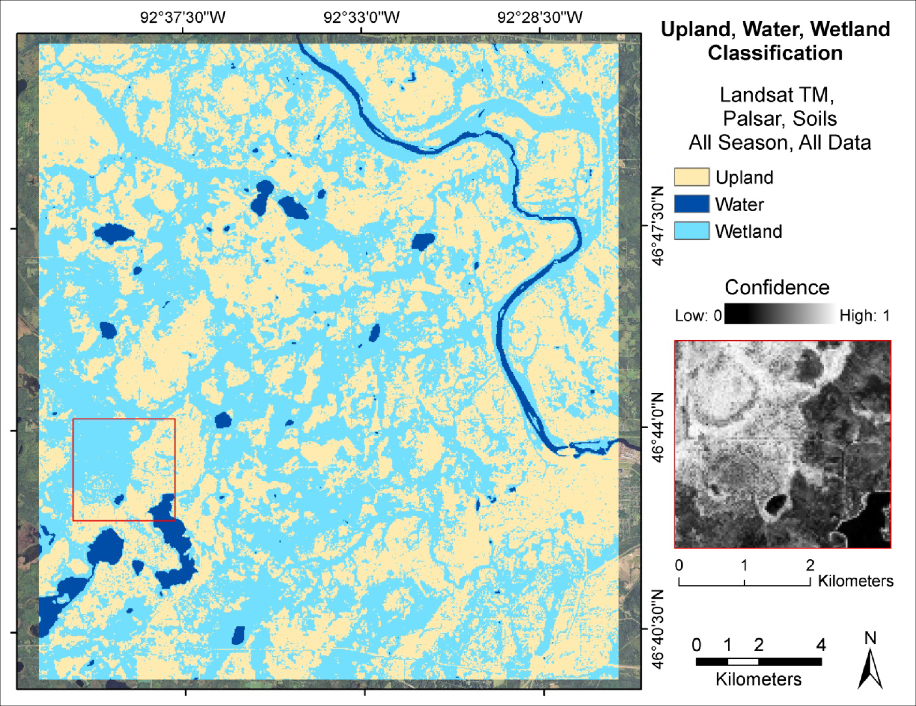
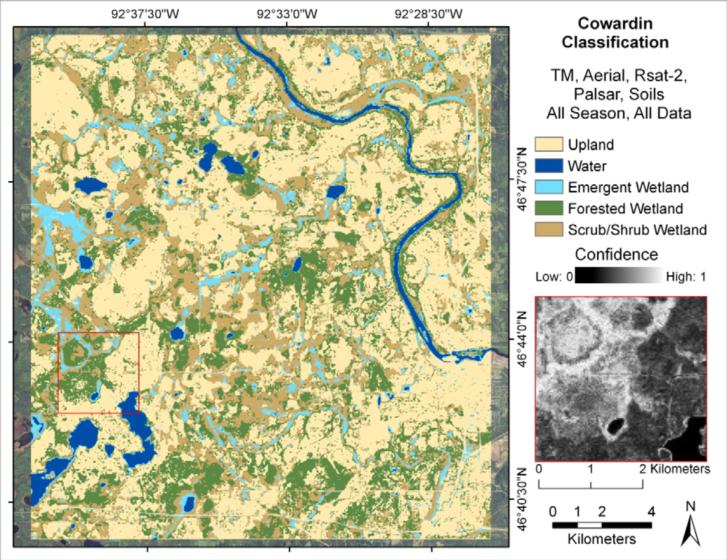
2.2. Land Cover Classification Schemes

Two levels of classification were performed. The land cover classification schemes we used differentiated between upland, water, and wetland areas (Level 1) and sub-classified wetlands into wetland type (Level 2). Upland areas included all non-wetland classes, for example: urban, forest, grassland, agriculture, and barren land cover classes. Areas classified as wetland were sub-classified into a modified version of the Cowardin classification scheme [44], including the three most common wetland classes in the study area according to the National Wetlands Inventory (NWI) [45]: emergent, forested, and scrub/shrub wetlands. We merged the palustrine unconsolidated bottom class with the emergent wetland class and the riverine unconsolidated bottom class with the water class, based on visual assessment of the landscape variability in the study area (Table 1).
Any errors present in the initial Level 1 classification result prior to sub-classifying the wetland class can be propagated to the Level 2 classification [4649]. We tested whether classification accuracy could be improved by developing a Level 2 classification directly from the full set of input data without first producing a Level 1 classification, but the results were too poor for further consideration. Thus, all subsequent Level 2 classification results and discussion represent a hierarchical sub-classification of the wetland class from the results of the corresponding Level 1 land cover classification.

2.3. Decision Tree Classification

We used random forest as the decision tree classifier for our study [50]. Generating decision trees was an efficient means of using our point reference training data to establish relations between our independent (remotely sensed and ancillary data) and dependent (field determined land cover class) variables to produce a land cover classification [51,52]. Random forest is a meta-classifier that consists of a collection (forest) of decision trees using training data. The decision trees were constructed with a random sample of input variables selected to split at each node [53]. The default number of variables selected equals the square root of the total number of input variables, which we held as a constant during forest growing. The decision trees were fully grown without pruning using a sample (with replacement) of about one-third of the training data. The cross-validation accuracy was calculated using the remaining training data (out-of-bag) and was used to evaluate the relative accuracy of each model prior to a formal accuracy assessment. Each tree produced a ‘vote’ for the final classification, where the final result was the class which had the highest number of votes [53]. The classification confidence, or probability, equals the ratio of the number of votes for a given class out of the total number of trees generated, with a resulting value range of 0–1. For each model tested we ran 500 decision trees.
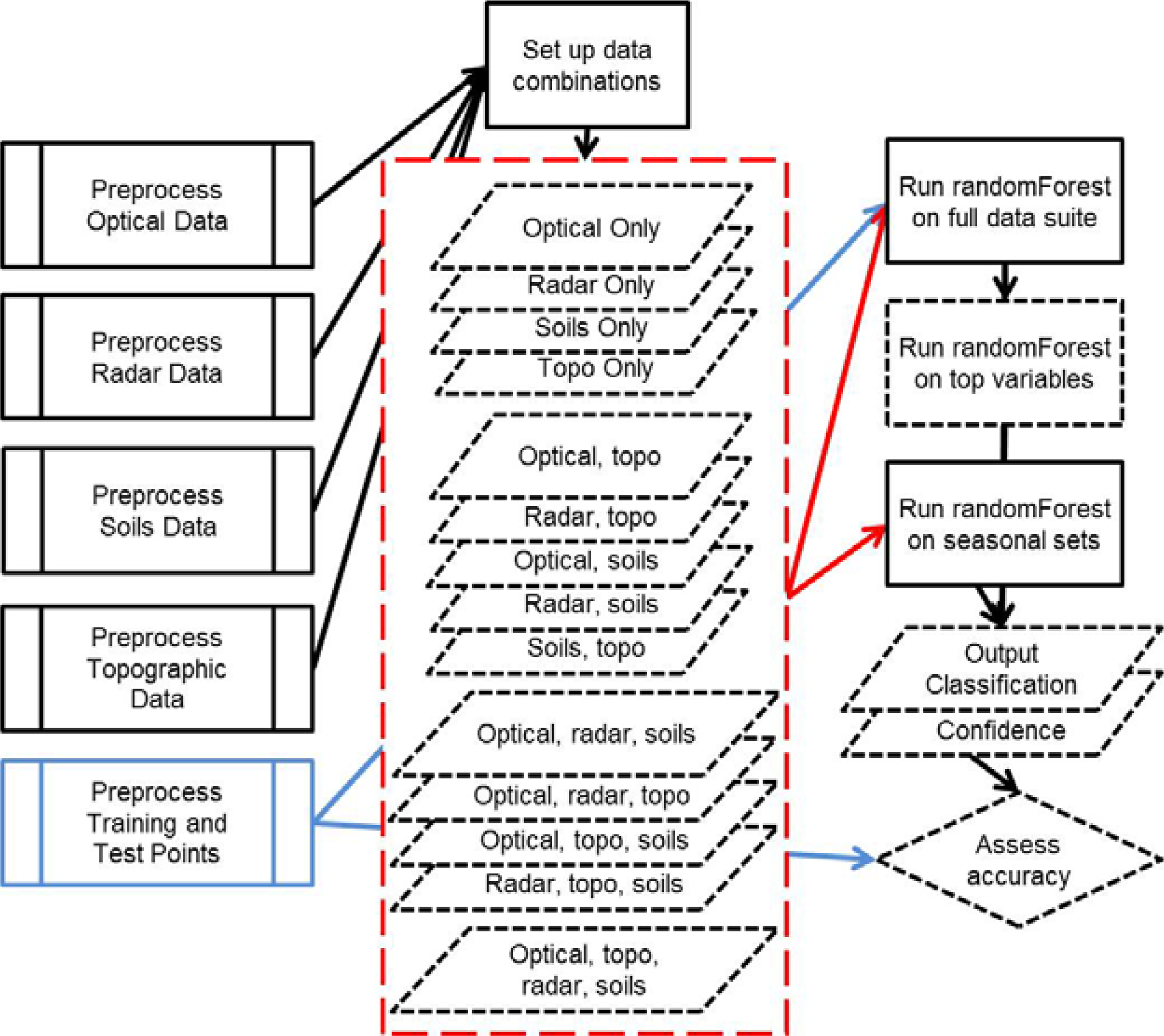
We built several random forest models per classification level by integrating different combinations of remotely sensed and ancillary input data to determine: (1) the most important data sources (corresponding to platform and wavelength of optical or radar data, and ancillary topographic and soils data derivatives), (2) the most significant input variables for mapping wetlands and classifying wetland type, and (3) the most effective temporal period (all data or only spring, summer, or fall season). Pre-defined combinations of input data are shown in Figure 2. We reviewed the top three models with highest overall accuracy for each classification level.
To determine if reducing the data load significantly changed the accuracy of the classification, we re-ran the top random forest models having the highest overall accuracy using only a selection of important variables-referred to as Reduced Data Load (RDL) models from this point forward. We used a combination of assessment measures from random forest (i.e., mean decrease in accuracy and Gini index for the overall model and per class, explained in the Accuracy Assessment section below) and expert knowledge to assess variable importance. In the selection of important variables for the RDL, we thought it was valuable to have fair representation from all data sources and seasons, to incorporate both remote sensing and wetland science knowledge, and to utilize the measures of variable importance produced by the random forest classifier. For example, if a radar data variable was within the top 20 variables for either the Gini index or the mean decrease in accuracy, that variable was included in the RDL model based on our knowledge of the sensitivity of the radar signal to saturated conditions. Selection for the Level 2 RDL was complex. We considered variable importance measures for the overall model and for each of the three wetland classes, and we incorporated expert knowledge of specific input data layers for our final selection of the RDL. We selected 10 important variables for the Level 1 classification. We increased our selection to 15 variables for the Level 2 classification to accommodate anticipated overlap in the input data distributions between different classes.

2.4. Training and Test Reference Point Data

Reference training and test point data (Table 2) were compiled from randomly generated field sites visited in the summers of 2009 and 2010, from study sites of an existing wetland monitoring program (centroids from polygons of the 2006–2008 MN Department of Natural Resources Wetland Status and Trends Monitoring Program [19]), and from our expert knowledge in photo interpretation. The protocol for reference data collection in 2009 and 2010 involved several steps in the field: two different field crews were sent to locate random ground reference points with a GPS unit; crew members identified the dominant Cowardin wetland type [44] within a reasonable visual distance; crew members recorded basic observations about the site’s characteristics; 2–5 photographs were taken per site; and crew members recorded the point ID, photo ID, Cowardin classification, and GPS coordinates in a back-up field book. Each field point represents a spatial area equal to the ground resolution of the input raster data used in the model (30 m). If the landscape surrounding the field point was not homogeneous within a reasonable visual distance, the field crew would use their discretion and move the GPS point to a new location which was more homogeneous. Empirical comparison of accuracies of results using different subdivisions of training and testing data [45] led us to use a stratified random sample of 75% of the reference point data for training the random forest classifier and 25% of the reference point data for testing the accuracy of the results. Reference points were added to the training dataset via photo interpretation to maintain appropriate representation of land cover classes and to preserve a suitable spatial distribution of training points. Assessment of outliers in the training dataset integrated the proximity measure from random forest (described in more detail below), aerial and field photo interpretation, and expert knowledge to determine whether training sites were appropriate reference for their respective classes. We filtered only training sites; all testing sites were maintained in the reference set (Table 2). Spatial autocorrelation in either reference dataset was not formally addressed in this study.
The set of reference training data were evaluated for outliers using the proximity measure from the random forest classifier. Proximity was calculated by running the training dataset down each tree in the forest a second time, increasing the proximity value by one each time the training site occupied the same terminal node of the decision tree in the first and second run. The proximity measure was normalized by dividing by the total number of trees generated by random forest. Training sites with a low proximity measure may be outliers in the training data. For this study, the proximity measure was used to guide the selection and evaluation of training sites that were considered outliers. Each of the identified sites was evaluated and, subsequently, some of the sites were removed.

2.5. Input Datasets and Process Flow

The implementation used to run random forest required that all raster data have the same spatial resolution and geographic extent. We chose to resample all raster data to match the layer with the coarsest resolution: Landsat 5 Thematic Mapper (TM) at 30 m spatial resolution. Resampling an image can introduce errors prior to classification [48], so we used the nearest neighbor sampling approach to minimize alteration of the original data values for our optical imagery. All input data were used in raster format and coregistered using ERDAS Imagine (v. 2010) with a root mean square error (RMSE) of less than 15 m.
In all of the tables and figures to follow, if a data source/platform is mentioned (e.g., “Landsat TM” or “radar”), all data layers from that source/platform are included in the tested combination. For example, the “All Season, All Data” model which uses Landsat TM, PALSAR, and Soils data includes all Landsat TM bands and derivatives from all dates (Table 2), all PALSAR polarizations from all dates, and all Soils data layers.
Following preparation of input datasets and training point data, we ran random forest to generate classification and confidence layers based on predefined combinations of datasets, including combinations of different platforms and seasons described earlier. We used our test point data to assess accuracy of each of the output classifications (Figure 2).

2.5.1. Topographic Input Data

We used the US Geological Survey (USGS) National Elevation Dataset (NED) [54] (10 m resolution resampled to 30 m) to determine elevation and derive slope gradient, aspect, curvature, and flow accumulation across the study area. The accuracy of this dataset varied spatially, but the overall vertical root mean square error was 2.44 m. We applied the flow accumulation function provided by the Environmental Systems Research Institute (ESRI) ArcGIS (v. 10.0) to calculate the direction(s) of water flow across the landscape and accumulate flow for all downslope cells. Cells with high flow accumulation imply areas of concentrated flow, such as stream channels, and cells with low flow accumulation likely are ridges or plateaus [55]. The curvature metric is a second derivative of slope and influences the convergence and divergence of water flow [23]. The topography of this study area does not vary significantly (330–450 m elevation, 392 m mean elevation, 20 m standard deviation; 0–37 degree slope with an average of 1.7 degrees). Compared to the height distribution of the study area, the vertical accuracy of the dataset has a negligible RMSE.

2.5.2. Soils Input Data

Soil attributes are defining variables in all working definitions of wetland areas [44]. Though soils data are not available everywhere and the quality of the maps that are available may be questionable, we tested the effectiveness of including or not including soils data in this study. We extracted soils tabular and vector data from the US Department of Agriculture (USDA) Soil Survey Geographic Data Base (SSURGO) [56]. The following data layers were used based on their likelihood to be associated with wetland areas: soil type (e.g., mucky peat, loam), dominant and wettest drainage class (e.g., moderately well drained, poorly drained, and somewhat poorly drained), and hydric class (e.g., hydric, or partially hydric) [25,57]. We joined the tabular and vector data for these four soils data layers and then converted the layers to raster format with 30 m spatial resolution.

2.5.3. Optical Input Data

Northern Minnesota is frequently cloudy, particularly in the summer, making it a challenge to find cloud-free conditions over our study area. The only Landsat TM imagery available with adequate cloud-free conditions was from early spring and fall (Table 3). We used blue (TM Band 1, B), green (TM Band 2, G), red (TM Band 3, R), near-infrared (TM Band 4, NIR), two mid-infrared (TM Band 5, MIR1; and TM Band 7, MIR2), and thermal infrared (TM Band 6, TIR) bands from all image dates. We included NIR, MIR1, MIR2, and TIR because of their suitability for land cover mapping and detecting water content in plants and soil [58,59]. Though multi-temporal and multi-platform data were used, the acquired satellite data were not atmospherically corrected and the data remained in digital number format. All of the input data were integrated into a single dataset, from which the training data were derived to classify land cover as a single snapshot [60].
We calculated both the normalized difference vegetation index (NDVI) and Tasseled Cap transformations for each TM image date. NDVI has been useful for separating vegetated versus non-vegetated areas and wet versus dry areas [61]. The brightness, greenness, and wetness axes of the Tasseled Cap transformation [62,63] have a long record of use in improving classification results, assessing land cover change, and aiding in estimates of forest structure and disturbance [6466].
Due to the aforementioned challenge to find cloud-free imagery during the summer season over our study area, we also acquired aerial orthophotos from the US Department of Agriculture (USDA) Farm Service Administration (FSA) National Agricultural Imagery Program (NAIP) for August 2008 and 2010 and an additional orthophoto from June 2009 (early leaf onset) to increase our temporal coverage of optical data during the summer season. The 2008 and 2009 images were acquired with visible and near infrared bands (blue, green, red, NIR), whereas the 2010 image was collected only in visible bands (blue, green, red). We used the red and near infrared bands to calculate NDVI for both 2008 and 2009. All aerial orthophotos were resampled to 30 m spatial resolution.

2.5.4. Radar Input Data

We used synthetic aperture radar (SAR) from RADARSAT-2 (C-band, 5.6 cm wavelength) and Advanced Land Observing Satellite (ALOS) Phased Array type L-band Synthetic Aperture Radar (PALSAR) (L-band, 23.6 cm wavelength) satellite systems (Table 4). We obtained two fully polarized RADARSAT-2 images (15 June 2009 and 19 September 2009) through the Canadian Space Agency’s Science and Operational Applications Research (SOAR) Program. Two additional dates (9 July 2009 and 26 August 2009) were made available by the Canada Center for Remote Sensing (CCRS). Though proprietary data and licensing restrictions prohibited us from incorporating the backscatter data from the dates provided by CCRS, we were able to generate polarimetric decompositions for use in our analysis (all preprocessing steps were performed in the same manner, described below). All of the RADARSAT-2 imagery was provided by the vendor with the constant beta application look up table (LUT) applied to avoid over saturation of the data [67]. Table 4 outlines which dates included the backscatter plus polarimetric decompositions (“Full dataset”) and which dates did not include backscatter (“Decomp only”).
We used the software package PCI Geomatica (v. 9.1) to preprocess the RADARSAT-2 imagery and generate polarimetric decompositions. Prior to resampling the imagery, we applied a boxcar filter (7 × 7 moving window) to reduce speckle and increase the number of effective looks for polarimetric decomposition [68]. The data were then resampled to 30 m using a mean window after terrain correcting the imagery. We then radiometrically corrected the data, performed antennae pattern correction, converted the amplitude values to sigma naught (σ0; output scaling LUT), and scaled the backscatter values in decibels for quantitative analysis [69]. After preprocessing the imagery as described above, we generated polarimetric decompositions.
We used three types of polarimetric decompositions on the RADARSAT-2 imagery to assess the benefits of radar polarimetry for mapping wetlands: van Zyl, Freeman-Durden, and Cloude-Pottier [70]. The premise behind a polarimetric decomposition is that the received signals contain important information regarding the structure of the landscape target, the scattering mechanism of the return signal, and the apparent shift in the phase of the signal from the target [7174]. The van Zyl decomposition is a classification [70] based on the backscatter and number of phase shifts that occur in the returned signal, where each pixel is discreetly classified as having a single, odd, or diffuse dominant backscatter. The Freeman-Durden decomposition [75] models the target scattering mechanisms as a continuous variable where each pixel represents relative proportions of surface scattering, double bounce, and volume scattering. The Cloude-Pottier decomposition [76] uses parameters of entropy, alpha angle, and anisotropy calculated from the eigenvalues and eigenvectors of a coherency matrix. Entropy is the randomness of scattering mechanisms, alpha angle represents the dominant scattering mechanism, and anisotropy characterizes directional dependence and importance of the secondary scattering mechanism. Among these three polarimetric decompositions, many authors have found the Freeman-Durden decomposition in particular to be useful for wetland mapping [7779]. These polarimetric decompositions represent the advanced analysis possible with radar polarimetry and thus were included in the random forest models which evaluated the effectiveness of RADARSAT-2 imagery for mapping wetlands.
We also acquired three dual-polarized (horizontal-horizontal (HH) and horizontal-vertical (HV)) ALOS PALSAR images (29 July and 11 September 2009 and 14 June 2010) for the study area from the Alaska Satellite Facility (ASF) archive (Table 4). We used the software package MapReady (v. 2.3), available through the ASF, for preprocessing the PALSAR data. The imagery was geocoded and resampled to 30 m spatial resolution using the default method, bilinear interpolation, which considers four neighboring pixel values. MapReady was used to perform antenna pattern correction using the beta coefficient, scale the data to decibel backscatter, and perform radiometric and geometric terrain correction using the 10 m NED elevation dataset. The RADARSAT-2 and PALSAR imagery were preprocessed using different LUTs and it is assumed that any resulting differences are negligible.

2.6. Accuracy Assessment

We reserved a stratified random subset of 25% of the reference point data and implemented traditional methods to assess accuracy and evaluate results. We constructed error matrices with overall accuracy, 95% confidence intervals (CI), User’s and Producer’s accuracies, kappa statistic (k-hat), and ran significance tests of error matrix k-hat values [80] for all random forest classification models. We performed two error matrix significance tests for each of the land cover classification levels: (1) between the most accurate random forest model with the full data suite to the same model with only a selection of the most important variables (RDL), and (2) between the most accurate random forest model with the full data suite to the most accurate random forest model using only data from a seasonal snapshot. Asterisks were used next to table values that were significant at an alpha of 0.05. We also conducted an accuracy assessment of the original NWI for comparison to our accuracy results.
Outputs from random forest provide unique complements to traditional accuracy assessment, including: (1) cross-validation, using the out-of-bag sample of training data to evaluate relative accuracy of each model prior to a formal accuracy assessment; (2) classification confidence, or probability, calculated by the number of times a given class was designated as the final class out of the total number of trees, with a resulting value range of 0–1; (3) mean decrease in accuracy, calculated per input data layer, giving insight to how influential a layer was on the overall accuracy; and (4) Gini index, which aids in evaluating the influence of input layers on the structure of the decision trees.
To calculate mean decrease in accuracy, the sample of reference data that was retained during the growth of each decision tree (out-of-bag) was used to determine the relative change in accuracy by including or excluding a particular variable. The normalized change in cross-validation accuracy was totaled after all decision trees were run and represents the relative importance of that variable [53]. The Gini index is calculated by, starting with an index value of 1, reducing the index value per variable every time that variable was used to make a dichotomous split in each decision tree. This index value was totaled per variable and represents the relative influence of that variable on the structure of each decision tree [53]. The most important variables in the random forest model can be inferred by evaluating both the mean decrease in accuracy and Gini index.

3. Results

3.1. Upland, Water, and Wetland Land Cover Classification (Level 1)

The most accurate full season random forest model for the Level 1 classification (85% accurate) integrated all available Landsat 5 TM, topographic, PALSAR, and soils data. The error matrix (Table 5) shows this model confused upland areas with wetland areas about 29% of the time (commission error calculated from the User’s accuracy), but wetland areas were confused with upland areas only 4% of the time. In terms of Producer’s accuracy (omission error), reference upland areas were more often correctly classified as uplands (94%) compared to the wetland class (78%). The water class was highly accurate in terms of both Producer’s and User’s accuracies (100% and 95%, respectively).
The second and third most accurate full season random forest models for the Level 1 classification had overall accuracies of 84% and 83%, respectively (Table 7). The second most accurate model incorporated all available Landsat 5 TM, aerial orthophoto, topographic, PALSAR, and soils data. This result shows that adding aerial orthophotos changes the accuracy by a very small amount (<1%). The third most accurate model incorporated all available Landsat 5 TM, topographic, RADARSAT-2, PALSAR, and soils data. This result shows that adding RADARSAT-2 data changes the accuracy by about 2%.
The classification map for the best Level 1 model illustrates how wetlands dominate the study landscape (Figure 3). The confidence for the resulting land cover classification (see representative area subset in Figure 3) was relatively high for most of the area classified as wetland, particularly around the shoreline of water bodies and in larger wetland complexes. Areas of lower confidence may be prone to misclassification from high variability or data redundancy in the input variables. We also tested a full season reduced data load (RDL) model to evaluate if using only the top 10 important variables significantly changed the accuracy of the classification.
We identified the top 10 variables using expert knowledge and the mean decrease in accuracy and Gini index values for each variable in the Landsat 5 TM, topographic, PALSAR, and soils model (Table 6). The overall accuracy of classification results from the RDL model (Table 7) was 81% (±4%) with generally lower values of Producer’s and User’s accuracies. However, a significance test of the difference between the full data suite and RDL models was not significant at an alpha level of 0.05. There was a small difference in the resulting wetland area between the two models: the full season model had a slightly lower total wetland area (18,969 ha) than the RDL model (19,010 ha). Though the difference in wetland area was negligible, a difference map of the results from the two models revealed widespread spatial differences, without pattern, due to more isolated pixels throughout the RDL model.
When ancillary datasets were used without the addition of remotely sensed data, the accuracy was significantly reduced. Classifying upland, water, and wetlands using topographic and soils data produced a higher accuracy (74%) than a model with soils data alone (73%) or topographic data alone (62%). Conversely, the best classification result without ancillary data, using only Landsat TM and PALSAR imagery, was still less accurate (80%) than models which used both remotely sensed and ancillary data (85%). All comparisons made here were statistically significant at an alpha level of 0.05. These findings show that integrating ancillary datasets with remotely sensed data can statistically improve accuracy of mapping wetlands.
We also evaluated results of different models from a temporal perspective to determine the influence of season for data acquisition on classification results (Table 8). Input data from different platforms were available for different periods of the growing season (Tables 3 and 4), a situation typical of multi-platform analyses and worth investigating. The seasonal model with the best accuracy (85%) was constructed from spring season data and had an overall accuracy comparable with the full season model. When we compared the full season and spring season models, the full season model had a lower total wetland area (18,969 ha) than the spring season model (19,679 ha). A difference map of the results from the two models did not reveal significant widespread spatial differences, but there was an observed pattern of differences occurring along roads and land cover transition zones; meaning, the two models have slight differences in feature boundaries. The most accurate model using fall data had an overall accuracy of 82% and the best model constructed from summer data had the least accurate results at 79%.

3.2. Cowardin Wetland Classification (Level 2)

The most accurate full season random forest model for the Level 2 classification integrated all available Landsat 5 TM, aerial orthophoto, topographic, RADARSAT-2, PALSAR, and soils data to yield an overall accuracy of 69% (±%5) (Figure 4). The overall accuracy for this model prior to sub-classifying the wetland class was 84% (±5%), with the Producer’s and User’s accuracies for the wetland class at 79% and 93%, respectively (±6% and 4%, respectively).
The error matrix for results from the best Level 2 classification model (Table 9) shows that upland areas were confused with wetland areas about 28% of the time (User’s accuracy was 72% ± 8%). The forested wetland class had the highest User’s accuracy (71% ± 13%) and the emergent wetland class had the highest Producer’s accuracy (65% ± 5%). Reference upland sites were classified correctly as uplands 92% of the time (±5%). Reference emergent wetlands were classified correctly 65% of the time (±5%), but forested and scrub/shrub wetlands were classified correctly only about half of the time (49% and 48%, respectively, ±12% for each). Both forested and emergent wetlands tended to be confused with scrub/shrub wetlands. The water class was highly accurate for both Producer’s and User’s accuracies (95% for each, ±11% for each).
The second and third most accurate full season random forest models for the Level 2 classification had overall accuracies of 66% and 65%, respectively (Table 10). The second most accurate model incorporated all available Landsat 5 TM, topographic, RADARSAT-2, PALSAR, and soils data. This result shows that when we do not include aerial orthophotos, the overall accuracy in sub-classifying wetlands changes by about 3%. The third most accurate model incorporated all available Landsat 5 TM, aerial orthophoto, topographic, RADARSAT-2, and soils data. This result shows that when we do not include PALSAR data, the overall accuracy in sub-classifying wetlands decreases by about 4%.
We assessed a full season RDL model to evaluate whether using the most important variables significantly changed the accuracy of the results for the Level 2 classification. We used expert knowledge and the mean decrease in accuracy and Gini index values for each variable in the full model to identify the top 15 variables for a RDL model (Table 11). The accuracy of the RDL model (Table 10) was 63% (± 5%), which did not differ significantly from the accuracy of the full model at an alpha level of 0.05. There was a difference in the resulting wetland area between the two models: the full season model had a lower total wetland area (18,351 ha) than the RDL model (20,376 ha). Most of the difference in area between the two models was from forested and scrub/shrub wetland classes erroneously classified as upland areas in the full season model. A difference map of the results from the two models revealed widespread spatial differences with an observed pattern of classification differences occurring along roads and land cover transition zones.
We evaluated several models to determine the extent to which season and corresponding data platforms could influence results for the most accurate Level 2 classification (Table 12). Satellite data from the spring yielded the most accurate results (71%), exceeding the level of accuracy produced by the full season model (69%). When we compared the full season and spring season models, the full season model had a higher total wetland area (18,351 ha) than the spring season model (17,162 ha). Most of the difference in area between these two models was from forested and scrub/shrub wetland areas erroneously classified as the upland class in the spring season model. A difference map of the results from the two models revealed less significant widespread spatial differences and no apparent pattern. The most accurate model using summer data had an overall accuracy of 65%. The best model constructed from fall data had the least accurate results at 62%.

4. Discussion

A key challenge in mapping and monitoring the landscape with remotely sensed data is that temporal coverage can be limited because of cloud contamination of imagery and because overpass schedules and return frequencies vary from platform to platform. Conditions for our research were no exception. This motivated us to examine the importance of type and seasonal timing of source data for classifying wetland-dominated landscapes in a forested region of the Upper Midwest.

4.1. Upland, Water, and Wetland Land Cover Classification (Level 1)

Our best Level 1 classification (85%) relied on ancillary soils, topographic, and remotely sensed data from satellite optical (Landsat 5 TM) and radar (PALSAR) platforms. This most accurate model used remotely sensed variables from fewer data sources than did the second (84%) and third best (83%) models, and did not require full temporal coverage (Table 7). A possible reason the best model did not place importance on summer data (aerial orthophotos), according to the Gini index and mean decrease in accuracy values, was that the fully developed tree canopy obscures underlying landscape features (i.e., inundation, wetland plant species, etc) that could otherwise reduce confusion in classifying vegetated upland and wetland areas [81]. The third most accurate model included RADARSAT-2 imagery and polarimetric decompositions, along with ancillary soils and topographic data. The fact that these particular radar datasets were not incorporated in the most accurate model implies that the C-band imagery was not as appropriate as L-band imagery for mapping wetlands in a forested region, primarily due to better propagation of the longer wavelength radar signal through the tree canopy. These results echo findings elsewhere that, though filtering techniques may vary, the high variability from radar backscatter in C-band imagery can confuse the model and cause a reduction in accuracy [34]. Though none of the three best models or the RDL model were significantly different from each other (at an alpha level of 0.05), all four models were significantly more accurate than the original NWI.
Reducing the number of variables in the Level 1 model to only the 10 most important variables produced results that were 4% less accurate than obtained with the full data suite model. However, this accuracy still was relatively high (81%) and enabled us to remove nearly 50 variables from the full model, thereby increasing classification efficiency and reducing cost without sacrificing a significant level of accuracy. Furthermore, our assessment of seasonal data sources suggests that imagery from spring alone can provide comparable results with imagery distributed throughout the entire growing season (Table 8). Most of the spring input data used in the model corresponded with above-normal precipitation conditions, confirming findings from other research that precipitation conditions are highly relevant to differentiating upland, water, and wetland classes [61,82]. Our results show the effectiveness of targeting input variables acquired during the spring season in this geographic region to improve land cover classification accuracy and confidence.
Results of the RDL model for this classification level showed that in addition to elevation, curvature, and hydric soils data, the most important spring season data included: satellite blue and NIR bands, satellite NDVI, and HV polarization using L-band radar. The satellite blue band, which had a high importance based on the mean decrease in accuracy for the upland class, was acquired on an especially clear day (17 April 2010) and thus had very little atmospheric interference, which typically makes this band noisy and not as useful. Others have found the blue band to be useful in classifying upland classes such as bare soil and in masking out shadowed areas [83,84]. Other studies have confirmed these remotely sensed variables, particularly near infrared and NDVI, are important for land cover classification and land cover change mapping. Such variables are particularly important when discriminating between forest structural condition (i.e., open or closed canopy), monitoring stand age and regrowth, and estimating species composition and richness [8587]. Studies have also established that the multiple scattering and subsequent depolarization of the radar signal explains the importance of HV polarization for classifying land cover and estimating biomass, particularly in forested regions [72,78,87]. It is important to note that even though our best results included ancillary soils and topographic input data, without the inclusion of ancillary data, the selected remotely sensed layers in the RDL model retain their level of importance.

4.2. Cowardin Wetland Classification (Level 2)

The second and third most accurate models (66% and 65%, respectively) developed for the Level 2 classification relied on fewer data sources than used by the best model and performed better than the RDL model. None of the three best models or the RDL model were significantly different from each other (at an alpha level of 0.05), but all four were a statistical improvement over the NWI (Table 10). Sub-classifying wetlands accurately required ancillary soils and topographic data, as well as increasing the temporal and spectral coverage of remotely sensed data with optical and L-band radar, the latter undoubtedly because of deeper canopy penetration and increased interaction of the signal which has been known to be useful for distinguishing differences in vegetative land cover [2628,88].
Our attempts to produce a RDL model using the top 15 variables from the full data suite indicated too great a reduction in classification accuracy for distinguishing between wetland types, even with the inclusion of ancillary soils and topographic data. The top 15 variables used in the model, though important, do not sufficiently represent the variation in characteristics needed to sub-classify wetlands. However, results from our seasonal analysis suggest output from a RDL model might be improved if we selected for spring data, as the spring model produced the highest accuracy for the Level 2 classification (Table 12).
We observed fewer differences from a visual comparison of results between the full season and spring models than between the full season and RDL models, but wetland class confidence was somewhat higher with full data suite (118 input data layers) than with the spring season model (33 input data layers). Though in some cases classification accuracy can be improved by increasing the number of input data layers [89], research has also shown that increasing the number of discrete classes requires comparable increases in training data to improve the sensitivity of classifiers to more refined class differences [90,91]. Results from our efforts to model Cowardin wetland classes indicate that our model might benefit from additional reference training sites, particularly for the forested and scrub/shrub wetland classes which had very low accuracy compared to the emergent wetland class.
The most important variables selected for a RDL model of the Level 2 classification incorporated a rather different set of data sources and seasons (Table 11) than were selected for the Level 1 classification (Table 6). The most important variables for sub-classifying wetlands included remotely sensed data from a broader temporal range than for simply differentiation between upland, water, and wetland areas. Many studies have found multi-temporal data to aid in land cover classification, particularly for wetland mapping [69,73,88,92]. The Level 2 model made use of thermal data and Tasseled Cap transformation derivatives, as well as a much greater use of radar data. Other studies have confirmed that thermal data is important for land cover classification, particularly in separating vegetated and impervious areas and different moisture levels throughout the landscape [58,93]. The Tasseled Cap transformation also has been used by others to improve wetland mapping [81,94]. We found that using radar backscatter was more useful than using the polarimetric decompositions; in particular, our findings further confirm those of others documenting the importance of co- and cross-polarization radar backscatter (HH and HV, respectively) in classifying land cover [9597].

5. Conclusions

One of our main goals was to identify an optimal selection of input data from various sources of remotely sensed and ancillary data to accurately map wetland areas in Northern Minnesota. We accomplished this goal by rigorously testing the results from several combinations of data at two classification levels. We found that the key input variables for accurately differentiating between upland, water, and wetland areas include satellite red, near infrared (NIR), and middle infrared (MIR1) bands and normalized vegetation index (NDVI), elevation and curvature, hydric soils ancillary data, and L-band horizontal-vertical (HV) polarization. We conclude that, in addition to the variables used for the Level 1 classification, the key input variables for a Level 2 classification of wetlands include Tasseled Cap Greenness and Wetness, satellite thermal band, and L-band horizontal-horizontal (HH) polarization. Our sound methods have generated an important set of results for the remote sensing community, describing in detail the differences in accuracy of wetland mapping in a forested region using specific data sources and combinations.
Weather conditions over the study site during the water years October 2007–September 2010 were relevant to conclusions made regarding seasonal data importance. This is because precipitation, and any subsequent deviation from the 30 year normal, influences the site’s hydrologic characteristics prior to data acquisition. The important spring datasets identified in Tables 5 and 9 all correspond to above normal precipitation conditions. With the exception of the summer of 2008, the rest of the important summer and fall datasets were acquired during below normal precipitation conditions. Though it is possible to plan spring data acquisition knowing the water year trends from the fall and winter before, it is difficult to fully anticipate precipitation events that will obscure optical data acquisition.
To accurately identify wetland areas in a forested region, such as Northern Minnesota, we found accuracy is improved when incorporating only spring season data for both Level 1 and Level 2 classifications. We conclude that, provided multi-temporal satellite optical, L-band radar (PALSAR), topographic, and soils data are included, identifying wetland areas in this region is more accurate when quad-polarization C-band radar (RADARSAT-2) and higher resolution aerial orthophotos are left out of the random forest model. However, we found that once wetland areas are identified, classifying wetland type is more accurate when C-band radar and broader temporal coverage of optical data are included. These findings are unique because through rigorous testing of different sources of remotely sensed data, a task that has not been done before in this region, we found that different wavelengths of radar data are beneficial for different levels of land cover classification.
The results of this study suggest that wetland mapping in a forested region such as Northern Minnesota can be improved by targeting the selection of important input variables from essential data platforms (such as L-band PALSAR) and by allocating more complete spectral coverage during the spring season. The way forward for further improvements to wetland classification in a forested region may include: analysis and utilization of classification confidence to target areas for future field reference data collection, using additional topographic information derived from light detection and ranging (lidar) such as canopy height and other parameters that relate to vegetation structure (e.g., standard deviation of height and number of returns within a grid cell, intensity), and incorporating spatial context and geometry of features through use of image segmentation and object based image analysis.

Acknowledgments

The authors gratefully acknowledge valuable assistance provided by Marvin Bauer of the University of Minnesota, Bruce Wiley of the US Geological Survey, and Rudi Gens of the Alaska Satellite Facility for their generous offer to review this manuscript. Funding for this research was provided in part by several sources and agencies: the Great Lakes Restoration Initiative and the US Fish & Wildlife Service; the Legislative Citizen Commission on Minnesota Resources, and the Environment & Natural Resources Trust Fund, and the Minnesota Department of Natural Resources; the Canadian Space Agency Science and Operational Applications Research (SOAR) Program and the Canadian Center for Remote Sensing; and the Alaska Satellite Facility and the Japan Aerospace Exploration Agency’s (JAXA) Japanese Ministry of Economy, Trade, and Industry (METI).

Conflict of Interest

The authors declare no conflict of interest.

References

  1. Vymazal, J. Constructed wetlands for wastewater treatment. Ecol. Eng 2005, 25, 475–477. [Google Scholar]
  2. Mitsch, W.J.; Gosselink, J.G. The value of wetlands: Importance of scale and landscape setting. Ecol. Econ 2000, 35, 25–33. [Google Scholar]
  3. Lane, C.R.; D’Amico, E. Calculating the ecosystem service of water storage in isolated wetlands using LiDAR in North Central Florida, USA. Wetlands 2010, 30, 967–977. [Google Scholar]
  4. Deschamps, A.; Greenlee, D.; Pultz, T.J.; Saper, R. Geospatial Data Integration for Applications in Flood Prediction and Management in the Red River Basin. Proceedings of IEEE International Geosciences and Remote Sensing Symposium and the 24th Canadian Symposium on Remote Sensing, Toronto, Canada, 24–28 June, 2002; pp. 3338–3340.
  5. Van der Kamp, G.; Hayashi, M. The groundwater recharge function of small wetlands in the semi-arid northern prairies. Wetlands 1998, 8, 39–56. [Google Scholar]
  6. Acharya, G.; Barbier, E.B. Valuing groundwater recharge through agricultural production in the Hadejia-Nguru Wetlands in Northern Nigeria. Agr. Econ 2000, 22, 247–259. [Google Scholar]
  7. Hamilton, S.K.; Kellndorfer, J.; Lehner, B.; Tobler, M. Remote sensing of floodplain geomorphology as a surrogate for biodiversity in a tropical river system (Madre De Dios, Peru). Geomorphology 2007, 89, 23–38. [Google Scholar]
  8. Richardson, D.M.; Holmes, P.M.; Esler, K.J.; Galatowitsch, S.M.; Stromberg, J.C.; Kirkman, S.P.; Pyšek, P.; Hobbs, R.J. Riparian vegetation: Degradation, alien plant invasions, and restoration prospects. Divers. Distrib 2007, 13, 126–139. [Google Scholar]
  9. Mayer, P.M.; Galatowitsch, S.M. Diatom communities as ecological indicators of recovery in Restored Prairie Wetlands. Wetlands 1999, 19, 765–774. [Google Scholar]
  10. Solomon, S.; Qin, D.; Manning, M.; Chen, Z.; Marquis, M.; Averyt, K.; Tignor, M.; Miller, H. Contribution of Working Group I to the Fourth Assessment Report of the Intergovernmental Panel on Climate Change; Cambridge University Press: Cambridge, UK, 2007. [Google Scholar]
  11. Hearne, R. Evolving water management institutions in the Red River Basin. Environ. Manage 2007, 40, 842. [Google Scholar]
  12. Environmental Laboratory, Corps of Engineers Wetlands Delineation Manual; Wetland Research Program; US Army Corps of Engineers: Vicksburg, MS, USA, 1987; p. Y-87-1.
  13. Wissinger, S.A. Ecology of Wetland Invertebrates. In Invertebrates in Freshwater Wetlands of North America: Ecology and Management; Batzer, D.P., Rader, R.B., Wissinger, S.A., Eds.; WIley: New York, NY, USA, 1999; pp. 1043–1086. [Google Scholar]
  14. Van der Sande, C.J.; de Jong, S.M.; de Roo, A.P.J. A segmentation and classification approach of IKONOS-2 imagery for land cover mapping to assist flood risk and flood damage assessment. Int. J. Appl. Earth Obs. Geoinf 2003, 4, 217–229. [Google Scholar]
  15. Ramsey, E.; Rangoonwala, A.; Middleton, B.; Lu, Z. Satellite optical and radar data used to track wetland forest impact and short-term recovery from Hurricane Katrina. Wetlands 2009, 29, 66–79. [Google Scholar]
  16. Nel, J.; Roux, D.; Abell, R.; Ashton, P.; Cowling, R.; Higgins, J.; Thieme, M.; Viers, J. Progress and challenges in freshwater conservation planning. Aquat. Conserv: Mar. Freshw. Ecosyst 2009, 19, 474–485. [Google Scholar]
  17. Mayer, A.L.; Lopez, R.D. Use of remote sensing to support forest and wetlands policies in the USA. Remote Sens 2011, 3, 1211–1233. [Google Scholar]
  18. Dahl, T.E. Wetlands Losses in the United States 1780’s to 1980’s; US Department of the Interior, Fish and Wildlife Service, Office of Biological Services: Washington, DC, USA, 1990; p. 13. [Google Scholar]
  19. Minnesota Department of Natural Resources. Wetlands Status and Trends. Available online: http://www.dnr.state.mn.us/eco/wetlands/wstm_prog.html (accessed on 20 August 2010).
  20. Haas, E.M.; Bartholomé, E.; Lambin, E.F.; Vanacker, V. Remotely sensed surface water extent as an indicator of short-term changes in ecohydrological processes in Sub-Saharan Western Africa. Remote Sens. Environ 2011, 115, 3436–3445. [Google Scholar]
  21. Goetz, S. Remote sensing of riparian buffers: Past progress and future prospects. J. Am. Water Resour. Assoc 2006, 42, 133–143. [Google Scholar]
  22. Dahl, T.E.; Watmough, M.D. Current approaches to wetland status and trends monitoring in Prairie Canada and the Continental United States of America. Can. J. Remote Sens 2007, 33, S17–S27. [Google Scholar]
  23. Moore, I.; Grayson, R.; Landson, A. Digital Terrain Modeling: A review of hydrological, geomorphological, and biological applications. Hydrol. Process 1991, 5, 330. [Google Scholar]
  24. Sader, S.A.; Ahl, D.; Liou, W. Accuracy of Landsat-TM and GIS rule-based methods for forest wetland classification in Maine. Remote Sens. Environ 1995, 53, 133–144. [Google Scholar]
  25. Li, R.; Zhu, A.; Song, X.; Li, B.; Pei, T.; Qin, C. Effects of spatial aggregation of soil spatial information on watershed hydrological modeling. Hydrol. Process 2012, 26, 1390–1404. [Google Scholar]
  26. Evans, T.L.; Costa, M.; Telmer, K.; Silva, T.S.F. Using ALOS/PALSAR and RADARSAT-2 to map land cover and seasonal inundation in the Brazilian Pantanal. IEEE J. Sel. Top. Appl. Earth Obs. Remote Sens 2010, 3, 560–575. [Google Scholar]
  27. Li, G.; Lu, D.; Moran, E.; Dutra, L.; Batistella, M. A Comparative analysis of ALOS PALSAR L-band and RADARSAT-2 C-band data for land-cover classification in a tropical moist region. ISPRS J. Photogramm 2012, 70, 26–38. [Google Scholar]
  28. Pereira, F.R.S.; Kampel, M.; Cunha-Lignon, M. Mapping of mangrove forests on the Southern Coast of São Paulo, Brazil, using Synthetic Aperture Radar data from ALOS/PALSAR. Remote Sens. Lett 2012, 3, 567–576. [Google Scholar]
  29. Bwangoy, J.B.; Hansen, M.C.; Roy, D.P.; Grandi, G.D.; Justice, C.O. Wetland mapping in the Congo Basin using optical and radar remotely sensed data and derived topographical indices. Remote Sens. Environ 2010, 114, 73–86. [Google Scholar]
  30. Castañeda, C.; Ducrot, D. Land cover mapping of wetland areas in an agricultural landscape using SAR and Landsat imagery. J. Environ. Manage 2009, 90, 2270–2277. [Google Scholar]
  31. Li, J.; Chen, W. Clustering Synthetic Aperture Radar (SAR) imagery using an automatic approach. Can. J. Remote Sens 2007, 33, 303–311. [Google Scholar]
  32. Bolstad, P.V.; Lillesand, T.M. Rule-based classification models: Flexible integration of satellite imagery and thematic spatial data. Photogramm. Eng. Remote Sensing 1992, 58, 965–971. [Google Scholar]
  33. Friedl, M.A.; Brodley, C.E. Decision tree classification of land cover from remotely sensed data. Remote Sens. Environ 1997, 61, 399–409. [Google Scholar]
  34. Li, J.; Chen, W. A rule-based method for mapping Canada’s wetlands using optical, radar and DEM data. Int. J. Remote Sens 2005, 26, 5051–5069. [Google Scholar]
  35. Pal, M.; Mather, P. An assessment of the effectiveness of decision tree methods for land cover classification. Remote Sens. Environ 2003, 86, 554–565. [Google Scholar]
  36. Rodriguez-Galiano, V.F.; Ghimire, B.; Rogan, J.; Chica-Olmo, M.; Rigol-Sanchez, J.P. An assessment of the effectiveness of a Random Forest classifier for land-cover classification. ISPRS J. Photogramm 2012, 67, 93–104. [Google Scholar]
  37. Naidoo, L.; Cho, M.A.; Mathieu, R.; Asner, G. Classification of savanna tree species, in the Greater Kruger National Park Region, by integrating hyperspectral and lidar data in a Random Forest data mining environment. ISPRS J. Photogramm 2012, 69, 167–179. [Google Scholar]
  38. Guo, L.; Chehata, N.; Mallet, C.; Boukir, S. Relevance of airborne lidar and multispectral image data for urban scene classification using Random Forests. ISPRS J. Photogramm 2011, 66, 56–66. [Google Scholar]
  39. Minnesota Department of Natural Resources. Natural History–Minnesota’s Geology. Available online: http://www.dnr.state.mn.us/snas/naturalhistory.html (on accessed 31 March 2011).
  40. United States Department of Agriculture. National Agricultural Statistics Service (NASS) Cropland Data Layer. Available online: http://www.nass.usda.gov/research/Cropland/SARS1a.htm (accessed on 31 March 2011).
  41. Minnesota Department of Administration (AdminMN). Office of Geographic and Demographic Analysis State Demographic Center, 2010 Census: Minnesota City Profiles. Available online: http://www.demography.state.mn.us/CityProfiles2010/index.html (accessed on 12 September 2012).
  42. National Oceanic and Atmospheric Administration. National Climatic Data Center (NCDC). Normals, Means, and Extremes for Duluth, MN. Available online: http://www.ncdc.noaa.gov/cdo-web/datasets/NORMAL_MLY/stations/GHCND:USW00014913/detail (accessed on 12 August 2012).
  43. Minnesota Department of Natural Resources. State Climatology Office, MN Climatology Working Group Historical Climate Data. Available online: http://climate.umn.edu/doc/historical.htm (accessed on 9 April 2012).
  44. Cowardin, L.; Carter, V.; Golet, F.; LaRoe, E. Classification of Wetlands and Deepwater Habitats of the United States; US Department of the Interior, Fish and Wildlife Service: Washington, DC, USA, 1979; pp. 1–79. [Google Scholar]
  45. United States Fish and Wildlife Service. National Wetlands Inventory (NWI). Available online: http://www.fws.gov/wetlands/ (accessed on 11 October 2011).
  46. Foody, G.M. Status of land cover classification accuracy assessment. Remote Sens. Environ 2002, 80, 185–201. [Google Scholar]
  47. Yuan, F.; Sawaya, K.E.; Loeffelholz, B.C.; Bauer, M.E. Land cover classification and change analysis of the Twin Cities (Minnesota) metropolitan area by multitemporal Landsat remote sensing. Remote Sens. Environ 2005, 98, 317–328. [Google Scholar]
  48. Lunetta, R.; Congalton, R.; Fenstermaker, L.; Jensen, J.; McGwire, K.; Tinny, L. Remote Sensing and Geographic Information System data integration: Error sources and research issues. Photogramm. Eng. Remote Sensing 1991, 57, 677–687. [Google Scholar]
  49. Janssen, L.L.F.; van der Wel, F.J.M. Accuracy assessment of satellite derived land-cover data: A review. Photogramm. Eng. Remote Sensing 1994, 60, 419–426. [Google Scholar]
  50. Liaw, A.; Wiener, M. Classification and Regression by randomForest. R News 2002, 18–22. [Google Scholar]
  51. Harken, J.; Sugumaran, R. Classification of Iowa wetlands using an airborne hyperspectral image: A comparison of the Spectral Angle Mapper classifier and an object-oriented approach. Can. J. Remote Sens. 2005, 31, 167–174. [Google Scholar]
  52. Hogg, A.R.; Todd, K.W. Automated discrimination of upland and wetland using terrain derivatives. Can. J. Remote Sens 2007, 33, S68–S83. [Google Scholar]
  53. Breiman, L. Random Forests. Machine Learn 2001, 45, 5–32. [Google Scholar]
  54. US Geological Survey. Accuracy of the National Elevation Dataset (NED). Available online: http://ned.usgs.gov/Ned/accuracy.asp (accessed on 10 March 2011).
  55. Tarboton, D.G.; Bras, R.L.; Rodriguez-Iturbe, I. On the extraction of channel networks from digital elevation data. Hydrol. Process 1991, 5, 81–100. [Google Scholar]
  56. Natural Resources Conservation Service, US Department of Agriculture. Soil Survey Geographic (SSURGO) Database for St. Louis and Carlton County, MN. Available online: http://soildatamart.nrcs.usda.gov (accessed on 1 September 2009).
  57. Zhu, Z.; Woodcock, C.E.; Rogan, J.; Kellndorfer, J. Assessment of spectral, polarimetric, temporal, and spatial dimensions for urban and peri-urban land cover classification using Landsat and SAR data. Remote Sens. Environ 2012, 117, 72–82. [Google Scholar]
  58. Baker, C.; Lawrence, R.; Montagne, C.; Patten, D. Mapping wetlands and riparian areas using Landsat ETM+ imagery and decision tree based models. Wetlands 2006, 26, 465. [Google Scholar]
  59. Shih, S.F.; Jordan, J.D. Landsat mid-infrared data and GIS in regional surface soil-moisture assessment. J. Am. Water Resour. Assoc 1992, 28, 713–719. [Google Scholar]
  60. Song, C.; Woodcock, C.E.; Seto, K.C.; Lenney, M.P.; Macomber, S.A. Classification and change detection using Landsat TM data: When and how to correct atmospheric effects? Remote Sens. Environ 2001, 75, 230–244. [Google Scholar]
  61. Ozesmi, S.L.; Bauer, M.E. Satellite remote sensing of wetlands. Wetlands Ecol. Manage 2002, 10, 381–402. [Google Scholar]
  62. Crist, E.P.; Cicone, R.C. A physically-based transformation of Thematic Mapper data—The TM tasseled cap. IEEE Trans. Geosci. Remote Sens 1984, 22, 256. [Google Scholar]
  63. Kauth, R.; Thomas, G. The Tasselled Cap—A Graphic Description of the Spectral-Temporal Development of Agricultural Crops as seen by Landsat. Proceedings of Symposium on Machine Processing of Remotely Sensed Data, West Lafayette, IN, USA, 29 June–1 July 1976; pp. 4B 41–51.
  64. Cohen, W.B.; Spies, T.A. Estimating structural attributes of Douglas-fir/western Hemlock Forest stands from Landsat and SPOT imagery. Remote Sens. Environ 1992, 41, 1–17. [Google Scholar]
  65. Dymond, C.C.; Mladenoff, D.J.; Radeloff, V.C. Phenological differences in tasseled cap indices improve deciduous forest classification. Remote Sens. Environ 2002, 80, 460–472. [Google Scholar]
  66. Jin, S.; Sader, S.A. Comparison of time series tasseled cap wetness and the Normalized Difference Moisture Index in detecting forest disturbances. Remote Sens. Environ 2005, 94, 364–372. [Google Scholar]
  67. Kaya, S. Personal Communication, Environment Canada, Canada Center for Remote Sensing; Ottawa ON, Canada, 30 June 2010. [Google Scholar]
  68. Bouchemakh, L.; Smara, Y.; Boutarfa, S.; Hamadache, Z. A Comparative Study of Speckle Filtering in Polarimetric Radar SAR Images. Proceedings of 3rd International Conference on Information and Communication Technologies: From Theory to Applications, Damascus, Syria, 7–11 April 2008; pp. 1–6.
  69. Parmuchi, M.G.; Karszenbaum, H.; Kandus, P. Mapping wetlands using multi-temporal RADARSAT-1 data and a decision-based classifier. Can. J. Remote Sens 2002, 28, 175–186. [Google Scholar]
  70. van Zyl, J. Unsupervised classification of scattering behavior using radar polarimetry data. IEEE Trans. Geosci. Remote Sens 1989, 27, 36–45. [Google Scholar]
  71. Henderson, F.M.; Lewis, A.J. Radar detection of wetland ecosystems: A review. Int. J. Remote Sens 2008, 29, 5809–5835. [Google Scholar]
  72. Baghdadi, N.; Bernier, M.; Gauthier, R.; Neeson, I. Evaluation of C-band SAR data for wetlands mapping. Int. J. Remote Sens 2001, 22, 71–88. [Google Scholar]
  73. Slatton, K.C.; Crawford, M.M.; Chang, L.D. Modeling temporal variations in multipolarized radar scattering from intertidal coastal wetlands. ISPRS J. Photogramm 2008, 63, 559–577. [Google Scholar]
  74. Wang, Y.; Davis, F.W. Decomposition of polarimetric Synthetic Aperture Radar backscatter from upland and flooded forests. Int. J. Remote Sens 1997, 18, 1319–1332. [Google Scholar]
  75. Freeman, A.; Durden, S. A three-component scattering model for polarimetric SAR data. IEEE Trans. Geosci. Remote Sens 1998, 36, 963–973. [Google Scholar]
  76. Cloude, S.; Pottier, E. An entropy based classification scheme for land applications of polarimetric SAR. IEEE Trans. Geosci. Remote Sens 1997, 35, 68–78. [Google Scholar]
  77. Corcoran, J.; Knight, J.; Brisco, B.; Kaya, S.; Cull, A.; Murnaghan, K. The integration of optical, topographic, and radar data for wetland mapping in Northern Minnesota. Can. J. Remote Sens 2011, 37, 564. [Google Scholar]
  78. Sartori, L.R.; Imai, N.N.; Mura, J.C.; Novo, E.M.L.M.; Silva, T.S.F. Mapping Macrophyte Species in the Amazon Floodplain wetlands using fully polarimetric ALOS/PALSAR data. IEEE Trans. Geosci. Remote Sens 2011, 49, 4717–4728. [Google Scholar]
  79. Brisco, B.; Kapfer, M.; Hirose, T.; Tedford, B.; Liu, J. Evaluation of C-band polarization diversity and polarimetry for wetland mapping. Can. J. Remote Sens 2011, 37, 82–92. [Google Scholar]
  80. Congalton, R.; Green, K. (Eds.) Assessing the Accuracy of Remotely Sensed Data: Principles and Practices, 2nd ed; CRC Press: Boca Raton, FL, USA, 2008; p. 200.
  81. Wright, C.; Gallant, A. Improved wetland remote sensing in Yellowstone National Park using classification trees to combine TM imagery and ancillary environmental data. Remote Sens. Environ 2007, 107, 582–605. [Google Scholar]
  82. Jensen, J.R.; Christensen, E.J.; Sharitz, R. Nontidal wetland mapping in South Carolina using airborne multispectral scanner data. Remote Sens. Environ 1984, 16, 1–12. [Google Scholar]
  83. Nobrega, R.A.; O’Hara, C.G.; Quintanilha, J.A. An Object-Based Approach to Detect Road Features for Informal Settlements near Sao Paulo, Brazil. In Object Based Image Analysis; Blaschke, T, Lang, S, Hay, G, Eds.; Springer: Heidelberg/Berlin, Germany, 2008; pp. 589–607. [Google Scholar]
  84. Doxani, G.; Siachalou, S.; Tsakiri-Strati, M. An object-oriented approach to urban land cover change detection. Int. Arch. Photogramm. Remote Sens. Spat. Inf. Sci. 2008, XXXVII, 1655–1660. [Google Scholar]
  85. Sesnie, S.E.; Gessler, P.E.; Finegan, B.; Thessler, S. Integrating Landsat TM and SRTM-DEM derived variables with decision trees for habitat classification and change detection in complex neotropical environments. Remote Sens. Environ 2008, 112, 2145–2159. [Google Scholar]
  86. Steininger, M.K. Tropical secondary forest regrowth in the Amazon: Age, area and change estimation with Thematic Mapper data. Int. J. Remote Sens 1996, 17, 9–27. [Google Scholar]
  87. Tuomisto, H.; Poulsen, A.D.; Ruokolainen, K.; Moran, R.C.; Quintana, C.; Celi, J.; Cañas, G. Linking floristic patterns with soil heterogeneity and satellite imagery in Ecuadorian Amazonia. Ecol. Appl 2003, 13, 352–371. [Google Scholar]
  88. Whitcomb, J.; Moghaddam, M.; McDonald, K.; Podest, E.; Chapman, B. Decadal Change in Northern Wetlands Based on Differential Analysis of JERS and PALSAR Data. Proceedings of 2009 IEEE International Geoscience and Remote Sensing Symposium, Cape Town, South Africa, 12–17 July 2009; pp. III-951–III-954.
  89. Carrão, H.; Gonçalves, P.; Caetano, M. Contribution of multispectral and multitemporal information from MODIS images to land cover classification. Remote Sens. Environ 2008, 112, 986–997. [Google Scholar]
  90. Jackson, Q.; Landgrebe, D.A. An adaptive classifier design for high-dimensional data analysis with a limited training data set. IEEE Trans. Geosci. Remote Sens 2001, 39, 2664–2679. [Google Scholar]
  91. Ho, T.K.; Basu, M. Complexity measures of supervised classification problems. IEEE Trans. Pattern Anal. Mach. Intell 2002, 24, 289–300. [Google Scholar]
  92. Townsend, P.A. Mapping seasonal flooding in forested wetlands using multi-temporal RADARSAT SAR. Photogramm. Eng. Remote Sensing 2001, 67, 857–864. [Google Scholar]
  93. Yang, L.; Huang, C.; Homer, C.; Wylie, B.; Coan, M. An approach for mapping large-area impervious surfaces: Synergistic use of Landsat-7 ETM+ and high spatial resolution imagery. Can. J. Remote Sens 2003, 29, 230–240. [Google Scholar]
  94. Baker, C.; Lawrence, R.; Montagne, C.; Patten, D. Change detection of wetland ecosystems using Landsat imagery and change vector analysis. Wetlands 2007, 27, 610–619. [Google Scholar]
  95. Augusteijn, M.F.; Warrender, C.E. Wetland classification using optical and radar data and neural network classification. Int. J. Remote Sens 1998, 19, 1545–1560. [Google Scholar]
  96. Hess, L.L.; Melack, J.M.; Filoso, S.; Wang, Y. Delineation of inundated area and vegetation along the Amazon Floodplain with the SIR-C Synthetic Aperture Radar. IEEE Trans Geosci. Remote Sens 1995, 33, 896–904. [Google Scholar]
  97. Hess, L.L.; Melack, J.M.; Novo, E.M.L.M.; Barbosa, C.C.F.; Gastil, M. Dual-season mapping of wetland inundation and vegetation for the Central Amazon Basin. Remote Sens. Environ 2003, 87, 404–428. [Google Scholar]
Figure 1. Study area near Cloquet, Minnesota (MN). The aerial photo on the right is from the 2008 National Agricultural Imagery Program (NAIP).
Remotesensing 05 03212f1
Figure 2. Data process flow. Preprocessing of input datasets and reference point data (shown in blue) are in the left-hand column. Combinations of datasets used to perform random forest (shown in red), along with generation of the output classification, confidence maps, and accuracy assessment are referenced by boxes in the right-hand column.
Remotesensing 05 03212f2
Figure 3. Output classification of the most accurate full season random forest model for the Level 1 land cover classification using all available Landsat 5 TM, topographic, PALSAR, and soils data.
Remotesensing 05 03212f3
Figure 4. Output classification of the most accurate full season random forest model for the Level 2 land cover classification using all available Landsat 5 TM, aerial orthophoto, topographic, RADARSAT-2, PALSAR, and soils data.
Remotesensing 05 03212f4
Table 1. Level 2 classification and our corresponding class modifications.
Level 2 ClassModification of the Classes Used
UplandUpland
WaterWater + Palustrine Unconsolidated Bottom
Emergent WetlandEmergent + Riverine Unconsolidated Bottom
Forested WetlandForested Wetland
Scrub/Shrub WetlandScrub/Shrub Wetland
Table 2. Summary of reference point data before and after the filtering of training sites.
Land Cover ClassificationTraining Sites Prior to FilteringFinal Sites for Model TrainingSites Used for Accuracy TestingFinal Total
Upland464305136441
Water69461965
Wetland421402149551

Total9547533041057

Emergent Wetland9710943152
Forested Wetland15614049189
Scrub/Shrub Wetland16815357210

Total421402149551
Table 3. Input optical data for decision tree classification.
SeasonDateBand CombinationsPlatform-Source
Spring17 April 2010B, G, R, NIR, MIR1, MIR2, TIRSatellite-Landsat 5 TM
19 May 2010B, G, R, NIR, MIR1, MIR2, TIRSatellite-Landsat 5 TM
June 2009B, G, R, NIRAerial Orthophoto-NAIP

SummerAugust 2008B, G, R, NIRAerial Orthophoto-NAIP
August 2010B, G, RAerial Orthophoto-NAIP

Fall21 September 2009B, G, R, NIR, MIR1, MIR2, TIRSatellite-Landsat 5 TM
4 October 2008B, G, R, NIR, MIR1, MIR2, TIRSatellite-Landsat 5 TM
Table 4. Input radar data for decision tree classification.
SeasonDateSourceAcquisition Mode *Incidence AngleProduct
Spring15 June 2009RADARSAT-2FBQ26.9 near, 28.7 farFull dataset
14 June 2010PALSARFBD34.3 centerFull dataset

Summer09 July 2009RADARSAT-2FBQ26.9 near, 28.7 farDecomp only
29 July 2009PALSARFBD34.3 centerFull dataset
26 August 2009RADARSAT-2FBQ26.9 near, 28.7 farDecomp only

Fall11 September 2009PALSARFBD34.3 centerFull dataset
19 September 2009RADARSAT-2FBQ26.9 near, 28.7 farFull dataset
*FBQ: Fine Beam Quad-polarization; FBD: Fine Beam Dual-polarization.
Table 5. Classification error matrix for the most accurate full season random forest model for the Level 1 classification which incorporated all available Landsat 5 TM, topographic, PALSAR, and soils data.
Reference Data

ClassUplandWaterWetlandRow TotalUser Accuracy (%)

Classified DataUpland9703913671
Water01811995
Wetland6014415096
Column Total10318184305

Producer Accuracy (%)9410078Overall = 85%
k-hat = 0.73, 95% CI ± 4%
Table 6. Top 10 important variables, in order of importance, selected from the most accurate full season random forest model used in a Reduced Data Load (RDL) model for the Level 1 classification.
Data TypeDateSource
NIR Band19 May 2010Landsat 5 TM
Hydric SoilsNAUSDA SSURGO
MIR1 Band21 September 2009Landsat 5 TM
ElevationNAUSGS NED
CurvatureNAUSGS NED
Green Band4 October 2008Landsat 5 TM
Red Band4 October 2008Landsat 5 TM
Blue Band17 April 2010Landsat 5 TM
NDVI17 April 2010Landsat 5 TM
HV Polarization14 June 2010PALSAR
Table 7. Error matrix summary of the three best full season random forest models for the Level 1 land cover classification, as compared to the NWI.
ModelOverall Accuracy (%)Kappa StatisticZ Statistic
Best: TM, topo, PALSAR, soils (Table 5)850.7319.4*
RDL: top variables in best model (Table 6)810.6716.3*
2nd Best: TM, aerial, topo, PALSAR soils840.7118.3*
3rd Best TM, topo, RSAT-2, PALSAR soils830.6817.2*
National Wetlands Inventory700.469.6*
*Values were significant at an alpha of 0.05.
Table 8. Summary of results for the best seasonal random forest models for the Level 1 land cover classification.
SeasonModelOverall Accuracy (%)Kappa StatisticZ Statistic
SpringTM, topo, PALSAR, soils850.7219.1*
SummerAerial, topo, PALSAR, soils790.6314.5*
FallTM, topo, RSAT-2, PALSAR, soils820.6716.3*
Full SeasonTM, topo, PALSAR, soils850.7319.4*
*Values were significant at an alpha of 0.05.
Table 9. Classification error matrix for the most accurate full season random forest model for the Level 2 classification which incorporated all available Landsat 5 TM, aerial orthophoto, topographic, RADARSAT-2, PALSAR, and soils data.
Reference Data

ClassUplandWaterEmergent WetlandForested WetlandScrub/Shrub WetlandRow TotalUser Accuracy

Classified DataUpland9804211413772
Water0181001995
Emergent Wetland51241124356
Forested Wetland30035114971
Scrub/Shrub Wetland10814345760
Column Total10719377171305

Producer Accuracy9294654948Overall = 69%
k-hat = 0.58
95% CI ± 5%
Table 10. Error matrix summary of the three best full season random forest models for the Level 2 classification.
ModelOverall Accuracy (%)Kappa StatisticZ Statistic
Best: TM, aerial, topo, RSAT-2, PALSAR, soils (Table 9)690.5816.4*
RDL: top variables in best model (Table 11)630.5013.7*
2nd Best: TM, topo, RSAT-2, PALSAR soils660.5515.3*
3rd Best: TM, aerial, topo, RSAT-2, soils650.5314.6*
National Wetlands Inventory550.3811.0*
*Values were significant at an alpha of 0.05.
Table 11. Top 15 important variables, in order of importance, selected from the most accurate full season random forest model used in a RDL model for Level 2 classification.
Data TypeDateSource
TC Greenness19 May 2010Landsat 5 TM
NDVI19 May 2010Landsat 5 TM
TIR Band17 April 2010Landsat 5 TM
MIR1 Band21 September 2009Landsat 5 TM
TC Wetness21 September 2009Landsat 5 TM
MIR1 Band4 October 2008Landsat 5 TM
HH Polarization21 September 2009PALSAR
HV Polarization21 September 2009PALSAR
NDVI17 April 2010Landsat 5 TM
NDVISummer 2008NAIP
TC Wetness19 May 2010Landsat 5 TM
TC Wetness4 October 2008Landsat 5 TM
HH Polarization14 June 2010PALSAR
HV Polarization14 June 2010PALSAR
HV Polarization29 July 2009PALSAR
Table 12. Error matrix summaries of the best seasonal random forest models for the Level 2 classification.
SeasonModelOverall Accuracy (%)Kappa StatisticZ Statistic
SpringTM, topo, PALSAR, soils710.6017.3*
SummerAerial, topo, soils650.5113.8*
FallTM, topo, RSAT-2, PALSAR, soils620.4813.0*
Full SeasonTM, aerial, topo, RSAT-2, PALSAR soils690.5816.4*
*Values were significant at an alpha of 0.05.

