Article

Global Biogeographical Pattern of Ecosystem Functional Types Derived From Earth Observation Data

1
Land Resource Management Unit, European Commission Joint Research Centre, I-21027 Ispra, Italy
2
Department of Geosciences and Natural Resource Management, Faculty of Science, University of Copenhagen, Oster Voldgade 10, DK-1350 Copenhagen, Denmark
*
Author to whom correspondence should be addressed.
Remote Sens. 2013, 5(7), 3305-3330; https://doi.org/10.3390/rs5073305
Submission received: 22 May 2013 / Revised: 27 June 2013 / Accepted: 1 July 2013 / Published: 10 July 2013
(This article belongs to the Special Issue Monitoring Global Vegetation with AVHRR NDVI3g Data (1981-2011))

Abstract

:
The present study classified global Ecosystem Functional Types (EFTs) derived from seasonal vegetation dynamics of the GIMMS3g NDVI time-series. Rotated Principal Component Analysis (PCA) was run on the derived phenological and productivity variables, which selected the Standing Biomass (approximation of Net Primary Productivity), the Cyclic Fraction (seasonal vegetation productivity), the Permanent Fraction (permanent surface vegetation), the Maximum Day (day of maximum vegetation development) and the Season Length (length of vegetation growing season) variables, describing 98% of the variation in global ecosystems. EFTs were created based on Isodata classification of the spatial patterns of the Principal Components and were interpreted via gradient analysis using the selected remote sensing variables and climatic constraints (radiation, temperature, and water) of vegetation growth. The association of the EFTs with existing climate and land cover classifications was demonstrated via Detrended Correspondence Analysis (DCA). The ordination indicated good description of the global environmental gradient by the EFTs, supporting the understanding of phenological and productivity dynamics of global ecosystems. Climatic constraints of vegetation growth explained 50% of variation in the phenological data along the EFTs showing that part of the variation in the global phenological gradient is not climate related but is unique to the Earth Observation derived variables. DCA demonstrated good correspondence of the EFTs to global climate and also to land use classification. The results show the great potential of Earth Observation derived parameters for the quantification of ecosystem functional dynamics and for providing reference status information for future assessments of ecosystem changes.

1. Introduction

There is growing evidence that ecosystem degradation is largely due to intensive human resource use together with increasing awareness of the dependence of the global population on the globe’s ecosystem services [13]. Ecosystem degradation arises from long lasting loss of vegetation cover and biomass productivity over time and in space [4], as result of a combination of natural/environmental and human/socio-economic drivers. The need for improved information on the status of lands and on degradation processes, along with standardized methodologies and understandable mapping, has to be addressed urgently. To tackle these complex global challenges, a monitoring and assessment system offering up-to-date information on the status and trends of ecosystem degradation and their causes and effects need to be developed. A useful monitoring and assessment system will supply indicators that account for the climate dependence of ecosystem functioning that is responsive to land cover and land use change while supplying knowledge of the temporal and spatial patterns of ecosystem dynamics at larger spatial scales. At global scales, such indicators are best derived from information on vegetation/land cover dynamics as core components to assess the state of ecosystem degradation [5]. In particular, various aspects of vegetation productivity and phenology dynamics, reflecting land cover/use transitions that might lead to ecosystem degradation, need to be considered in a spatio-temporal context [6].
The Local Net Primary Productivity Scaling (LNS) approach relates actual ecosystem degradation to the potential degradation of ecosystems [7,8] where remote sensing estimated productivity of each pixel is expressed relative to the 90 percentile observed in all pixels falling within the same homogeneous ecosystem unit. Thus the LNS method requires the characterization of ecosystem units with similar biomass production potential, which might be defined by biophysical information on vegetation, soils, terrain and climate [7]. Besides this biophysical information ecosystems may be also characterized by the physiognomy and functional dynamics of the vegetation cover. Plant Functional Types (PFTs) are characterized by the physiognomy and functional dynamics of the vegetation and thus offer a possible framework for the identification of such homogenous ecosystem units providing a powerful tool in global change research [911]. This is because PFTs summarise the complexity of individual species and populations in recurrent patterns of plants that exhibit similar responses to biophysical environmental conditions. Hence, PFTs bridge the spatial and functional gap between plant physiology, land biophysical properties and ecosystem processes. Furthermore, identifying PFTs enables the assessment of ecosystem functions that might support predicting ecosystem response to human-induced changes [12], because the functional composition of PFTs changes in response to human disturbances [13,14] as well as in response to global change of ecosystems [15]. During the last decades the concept of Ecosystem Functional Types (EFTs) was developed for global scale assessment of ecosystems mostly based on the concept of PFTs, being defined as land surface areas with similar productivity (carbon gain/loss) dynamics.
Because of the large areal coverage and continuous temporal sampling, remotely sensed data provides a synoptic representation of vegetation dynamics in space and time and thus have a great potential for the assessment of ecosystems from regional to global scales [16]. Satellite derived vegetation indices, such as the NDVI, have proven their value in the field of large scale monitoring of vegetation cover and dynamics for land degradation and desertification studies (for an overview see [4,7,17]). Especially the de-convolution of the original time series into phenological and productivity metrics yield additional information on various aspects of vegetation dynamics and ecosystem functioning [18] that can be related to land use [19]. Monitoring vegetation phenology using satellite remote sensing [2025] offers an optimal framework for ecosystem studies because in situ phenological data are comparatively scarce in many parts of the world [26] and because long time and large spatial scales can be addressed simultaneously. Monitoring vegetation phenology has also improved the understanding of the interactions between the biosphere, the climate and biogeochemical cycles [16,2729]. Lloyd [30] has proposed the use of remote sensing derived phenology for the description of ecosystem functioning whereas Soriano and Paruelo [31] proposed the classification of biozones for the assessment of EFTs based on the seasonal dynamics of vegetation indices derived from satellite observations. Using remote sensing for the evaluation of the functional components of the ecosystems and the characterisation of EFTs has been gaining importance in recent decades (see [32] for a thorough review).
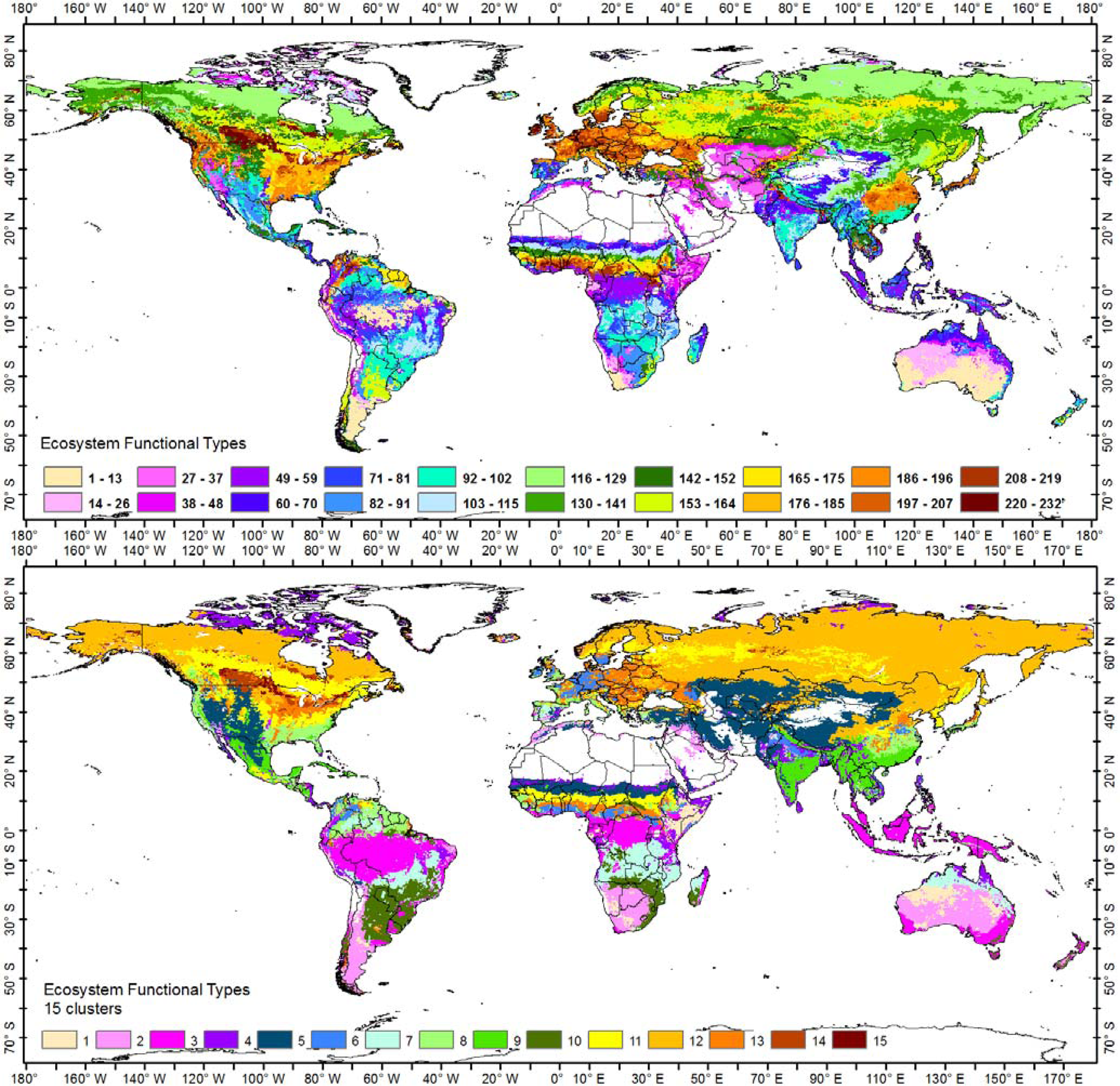
There is a need for quantitative methods to map the status and/or change of ecosystem services and thus supplying a standardized framework for ecosystem degradation studies. Therefore, in the present study we aim at identifying global EFTs [12,3134] in order to supply ecosystem degradation studies relating actual to potential degradation with homogenous biophysical units such as the LNS method [8]. In our study, EFTs are defined as spatial units with similar patterns of seasonal phenology and productivity dynamics, also showing similar responses to changing natural and human induced environmental conditions following the ideas of Paruelo et al. [12] and Stow et al. [
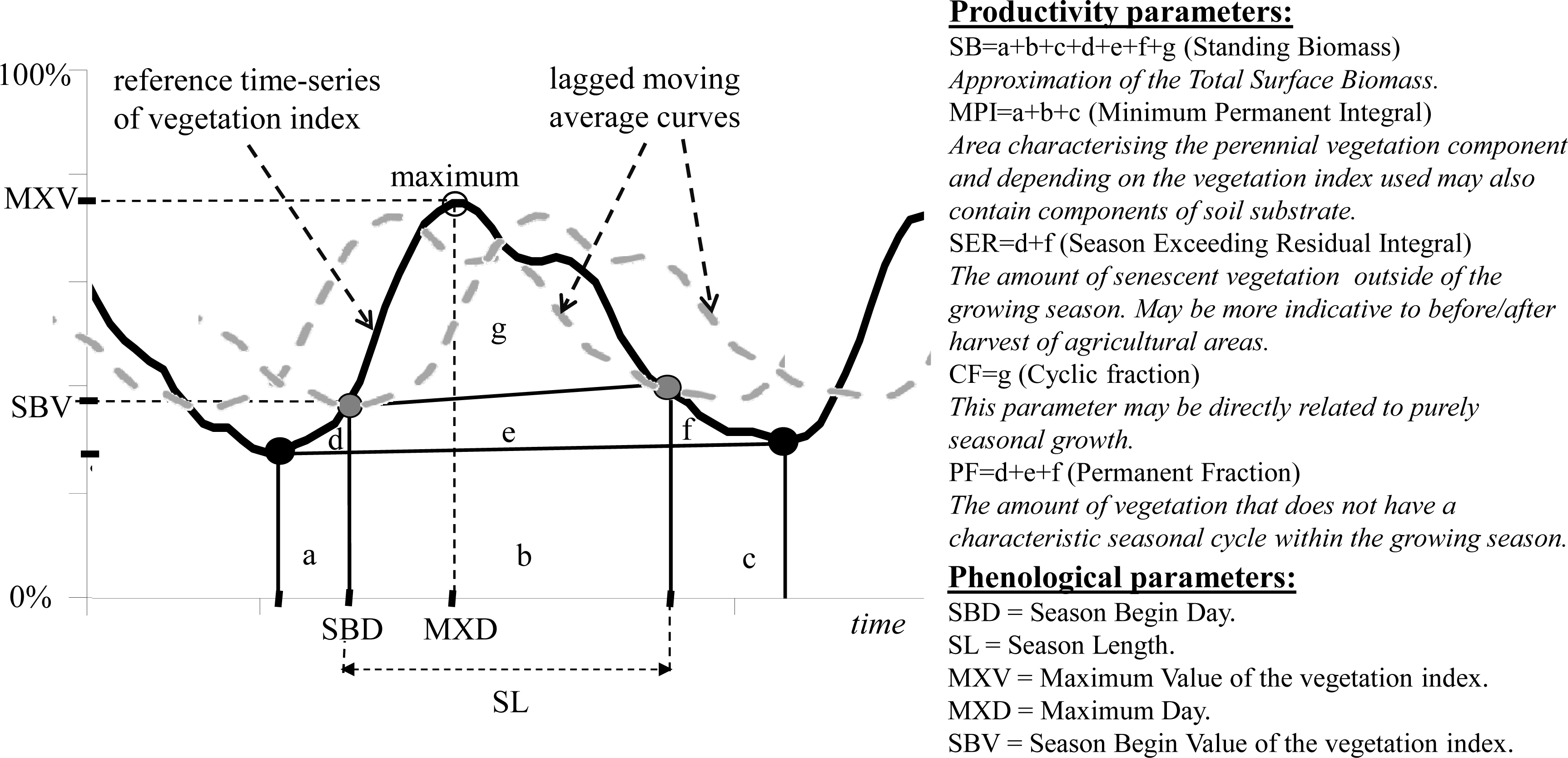
34]. Seasonal phenological and productivity dynamics are calculated from the GIMMS3g NDVI time-series (1982–2010) by decomposing the yearly NDVI signal into various metrics. Since we describe the functioning of global ecosystems within large climatic and biophysical gradients we derived a larger set of parameters indicating vegetation seasonal dynamics when compared to Paruelo et al. [12] and Alcaraz-Seguera et al. [3537]. As human activities such as abrupt land cover/land use change also play a significant role in land degradation processes [7], EFTs should also relate to land use. Therefore, when characterising ecosystems, a compound set of functional attributes that describe vegetation dynamics should also be included. We illustrate that the global EFTs reflect climate and land use and therefore offer a meaningful, transparent and objective stratification for global ecosystem monitoring studies.

2. Data and Methods

2.1. Data

The Normalised Difference Vegetation Index (NDVI) dataset was acquired from the Global Inventory Modeling and Mapping Studies (GIMMS) project. The dataset covers the period July 1981 to December 2011 and is produced as bi-monthly maximum-value composite (MVC) NDVI images referred to as NDVI3g (third generation GIMMS NDVI). The channel 1 and 2 data used for the GIMMS data are calibrated as suggested by Vermote and Kaufman [38], and the derived NDVI is further adjusted using the technique of Los [39]. The NDVI3g applies an improved cloud masking as compared to older versions of the GIMMS dataset and the cloud detection algorithm is based on reflectance and brightness temperature values [39,40]. No atmospheric correction is applied to the GIMMS data except for volcanic stratospheric aerosol periods (1982–1984 and 1991–1994) [41]. A satellite orbital drift correction is performed using an empirical mode decomposition/reconstruction (EMD) method of Pinzon et al. [42] minimizing effects of orbital drift by removing common trends between time series of solar zenith angle (SZA) and NDVI. The GIMMS3g NDVI data is provided in 1/12-degree resolution. Only vegetated areas were included in the present study by masking out pixels with a standard deviation of NDVI values below 0.02 [43].
In different parts of the world temperature, radiation, and water interact to impose complex and varying limitations on vegetation activity [44]. In order to assess these limitations over the derived EFTs, global climatic plant growth constraints [29] were included in the present study. These climatic plant growth constraint data were created from long-term climate statistics and includes gridded information of the relative importance of water availability (wat), air temperature (temp) and incoming shortwave radiation (rad) for vegetation across the globe. In order to demonstrate the correspondence of the EFTs in relation to climatic zones the updated Köppen-Geiger classification was acquired for the study [45]. Information on land use and management is also indispensable if the goal is to understand global environmental change and the loss of ecosystem services. Only a few global databases are available that allow the characterization of the land management concentrating on irrigation, the presence of livestock and of protected areas. In order to address land use and management on the global scale the present study utilized the Land Use Systems (LUS) maps of the world produced by the United Nations Food and Agricultural Organization [46]. The LUS classification includes several layers as the Global Land Cover dataset (GLC 2000), agro maps indicating cropping patterns (e.g., dominant crop types), livestock data, major ecosystem types, biophysical resources base layers (e.g., temperature regime, length of growing period, dominant soil units and terrain information) and socio-economic attributes.

2.2. Derivation of Phenological and Productivity Parameters

Phenological and productivity parameters were derived using the Phenolo software developed in the EC Joint Research Centre [19]. In order to generate results comparable between data sources with different time aggregation windows, daily values were calculated by an iterative linear interpolation of the NDVI time-series decades. Subsequently, a Savitzky-Golay filter with fourth polynomial degrees and a length of 50 days was applied to the time series in order to identify and remove short peaks and drop-offs caused by noise. This pre-processing resulted in the reference time series on which a set of phenological and productivity parameters were computed. The methodology is based on computing a delayed and a forward shifted time-series using a moving average filter and extracting the intersection points of these with the reference time-series. While Reed et al. [47] determined a general lag based on a priori knowledge about the average phenology of the study area, Phenolo is strictly data driven using for each individual pixel its time series dynamics to determine the lag in order to render it applicable to a wide geographical extent (see [19] for a complete description of the method). Once the intersection points are defined a series of phenological and productivity metrics were computed for each year in the time-series (see Figure 1).

2.3. Statistical Screening of the Phenological and Productivity Parameters

The yearly phenological and productivity variables were summarized in their temporal mean (1982–2010) and consecutively screened for multicollinearity based on the correlation matrix. Variables with very high correlation (>0.7) were removed from the analysis. Principal Component Analysis (PCA) was run on the Phenolo variables using the correlation rather than the covariance matrix in order to standardize the remote sensing variables with different measurement scales. This first, “screening PCA” served for (1) the selection of that set of Principal Components (PC) that explained the highest amount of total variance in the Phenolo variables and (2) for the selection of those Phenolo variables that showed the highest loadings on the selected components. The loadings of the individual variables were normalized by multiplication with the square root of the eigenvalues in order to present the values as correlation with the PCA axes. Once the n number of Principal Components was determined and the remote sensing variables with the highest loadings were selected, the “final PCA” was run on the selected n number of variables extracting n number of axes. The PCs were rotated with the “varimax” technique [48] in order to clearly associate each PC axes with one Phenolo variable only. The spatial patterns of the final rotated components were calculated by multiplying the loadings with the selected phenological variables.

2.4. Classification of Global Ecosystem Functional Types Based on the Phenological and Productivity Parameters

An ISODATA cluster analysis was used to identify major Ecosystem Functional Types (EFTs) at global scale. The analysis was run on the spatial patterns of the final rotated components because the PCA with correlation matrices normalized the eigenvectors with zero mean and 1 SD. This is a statistical property desirable for the calculation of class means evenly distributed in the data space and for the iterative clustering of the pixels using minimum distance techniques. Several test runs showed that if the range of the number of classes requested was allowed to be large (min = 10 and max = 500) the number of iterations had the highest influence on the resulting number of clusters. The algorithm was run 15 times where for each run the number of iterations increased with 1 (from 1 to 15) and another 5 times with 20, 25, 30, 50 and 100 iterations. We used discriminant analyses on the resulting EFTs of the 20 ISODATA classification runs to assess the number of EFTs best separated by the rotated eigenvectors. For each discriminant analysis we calculated the Wilks’ lambda and the canonical correlation. The former is a multivariate test of significance, where values close to 0 indicate that the group means are different whereas values close to 1 indicate similar group means. The canonical correlations of the discriminant functions indicate the proportion of total variability explained by differences between the groups. We have selected the ISODATA iteration run for which the Wilks’ lambda measure was lowest and the canonical correlation was highest. This run created EFTs significantly different in their phenology and productivity. To facilitate summarizing and reporting results the EFTs were further classified into a smaller number of clusters. For this, the rotated eigenvectors were spatially averaged within the EFTs and submitted to a dendrogram analysis joining EFTs into clusters such that the variance within the clusters was minimized. The sum of squared deviations was used as a measure for an EFT to enter the cluster, i.e., an EFT entered a cluster if its inclusion in the cluster produced the least increase in the error as measured by the sum of squared deviations.

2.5. Relation of the EFTs to the Phenological and Productivity Parameters and to Climatic Vegetation Growth Constraints

In order to characterize the EFTs in terms of their vegetation productivity and phenology dynamics a gradient analysis was run using another PCA (gradient PCA). The input for this analysis was a data table with the EFTs as rows and the Phenolo variables (selected through the screening PCA and final PCA analysis) averaged within the EFTs as columns. The data was centered and standardized to bring the variables to the same measurement scale. Redundancy Analysis (RDA) was used to assess the association of the EFTs and their phenological and productivity values with the climatic vegetation growth constraint variables (water, temperature and radiation). These variables were also averaged within the EFTs and added to the data table as columns. The significance and F-value of the RDA run was determined with the Monte-Carlo permutation test with 999 permutations. The association of the EFTs, Phenolo variables and climatic constraints were presented in a PCA tri-plot instead of an RDA tri-plot. This indicates correlation of the variables, rather than the variance the climatic variables explain, and thus facilitates focusing interpretation of results on the EFTs. The climatic and Phenolo variables were presented by arrows. Arrows pointing in the same direction in the tri-plot indicate positive correlation of the variables whereas arrows closing an approx. 90 degree indicate no correlation between the variables. The EFTs were represented by different icons depending on the clusters they were classified to with the dendrogram analysis. Projecting the EFTs perpendicularly onto one of the arrows of the Phenolo or climatic variables shows the value of the variable in that EFT. This tri-plot interprets the EFTs with vegetation phenological and productivity dynamics and additionally demonstrates the correlation of the Phenolo variables and the EFTs with the climatic constraints. Finally, to visualize the relationship of the EFTs with the remote sensing derived vegetation phenology and productivity variables the PCA values of the EFTs along the first two PCA axes were mapped. The relationship of the EFTs with radiation, temperature and water constraints of vegetation growth was visualized by mapping the RDA values of the EFTs along the first two RDA axes.

2.6. Relation of the EFTs to Global Climate and Land Use Classifications

In order to correlate the EFTs of the ecosystems with existing global classifications Detrended Correspondence Analysis (DCA) was carried out with the Köppen climate zones and with the FAO Land Use System classes (Table 1), respectively. The LUS classes were intersected with the major climate zones Tropical (Tr), Arid (Ar), Temperate (Tm), and Cold (Cd) in order to better describe the climate dependent seasonal dynamics of LUS classes. The input for the analysis was a data table with the EFTs as rows and the number of pixels belonging to the Köppen zones respectively to the LUS classes within the given EFTs as columns. The DCA axes were detrended by second order polynomials in order to avoid the arch effect caused by the strong environmental gradients [49] and for better interpretability of the ordination tri-plot. The tri-plots of the first two DCA dimensions were presented plotting the EFTs, the Köppen zones respectively the LUS classes and the selected Phenolo variables. Close Euclidean distances between the spatial units of the EFTs and the Köppen classes respectively the FAO land use classes indicate good correspondence with the EFTs. The spatial patterns of the DCA ordinations were presented in maps plotting the distance of each EFT from the center of the biplot. These maps further facilitated the interpretation of the DCA tri-plots. In order to find EFTs with low correspondence to the Köppen zones and LUS classes respectively, the percentage of fit of each EFTs in the ordination space was mapped by calculating the chi-square distance between the EFTs and the centroid of all samples.

3. Results

3.1. Statistical Screening of the Phenological and Productivity Parameters

The first five rotated axes of the screening PCA (10 input variables as in Figure 1) explained 98.6% of the variation in the global ecosystems (Table 2). The first axis alone explained 41.1% of the variation while the second, third, fourth and fifth axes explained 19.4%, 17.4%, 12.5% and 8.2%, respectively. The final PCA was run with the five variables loading highest on the first five rotated axes: Standing Biomass (SB), Cyclic Fraction (CF), the Maximum Day (MXD), the Season Length (SL) and the Permanent Fraction (PF) (Figure 1). Standing Biomass and Maximum Day have been used in other studies and are similar to EVI mean, NDVI sum and DMAX [10,32,33], while the other variables are new, extending the available set of phenological and productivity metrics in view of characterizing global EFTs. Some differences between the global distribution of the Standing Biomass as a productivity measure calculated in this study and spatial results from other productivity models (for a review see [48]) are partly due to the different nature of the methods. Standing Biomass is a yearly integration of all observed above ground biomass whereas NPP models are based on the fixation rate of atmospheric CO2. The Cyclic Fraction, representing a rate of annual active biomass growth, is highest over high latitude areas with frequent snow cover. This reflects the very strong intra-annual dynamics of seasonal vegetation cover that starts from very low values due to snow cover. Low Cyclic Fraction values are observed over areas either without seasonal snow cover or with very low Standing Biomass (arid areas) or over evergreen vegetation cover lacking yearly greening up dynamics. The Season Length presented in this study and Length of Growing Period (LGP) presented in other studies [50,51] are of different nature. The Season Length variable reflects a full growth cycle of all observed standing vegetation whereas LGP data models refer to the number of days when temperature and moisture conditions are considered adequate for crop growth. On the other hand, short EO-derived Season Length values over the African tropical forest possibly relate to persistent cloud cover affecting satellite data quality in the visible bands. Furthermore, the Maximum Day variable did not consider areas with double or multiple growing seasons and future studies should consider the proper characterization of such territories.
In the final PCA run, the first rotated axis explained 21.2% of the total variance (Table 2) and was mostly associated with the Standing Biomass of the global ecosystems (strongest positive loading, Table 3). The second PCA axis also explained 20.4% of the variation and was associated with the Season Length. The third rotated PCA axis was mostly related to the timing of the NDVI maximum (MXD) of the ecosystems and it explained 20.3% of the variance. The fourth rotated PCA axis was mostly dominated by the Cyclic Fraction explaining 19.9% of the variance whereas the fifth rotated axis represented an environmental gradient dominated by the Permanent Fraction explaining 18.2% of the variation in the data. The Isodata cluster analyses of the spatial pattern of the rotated Principal Components reached highest significance (Wilk’s lambda of 0.121 and canonical correlation of 0.937) at the 10th iteration. This iteration resulted in the creation of 232 global EFTs with significantly different group means and with a high percentage of variance of the rotated Principal Components explained. The 232 EFTs were subsequently regrouped into 15 major categories based on minimizing the variance of the rotated eigenvectors within the EFTs and maximizing the variance between them (Figure 2).

3.2. Relation of the EFTs to the Phenological and Productivity Parameters

The first two axes of the gradient PCA ordination explained 79.1% of the variance in the phenological and productivity variables and widely spanned the EFTs indicating good description of the global environmental gradients (Figure 3). The arrows of Standing Biomass and Permanent Fraction point to the same part of the triplot at the positive end of the first gradient PCA axis (clusters 6, 8, 13 and 14) indicating that EFTs with high Standing Biomass tend to have higher Permanent Fractions than the EFTs in other clusters. The Cyclic Fraction and the Maximum Day is almost perpendicular to Standing Biomass indicating that their values appear to be independent at global scale.
Thus, EFTs with high positive scores on the first PCA axis exhibit high Standing Biomass, high Permanent Fraction, longer seasons whereas the timing of their yearly maximum and their Cyclic Fraction can take a large range of values. These EFTs are mapped with high positive values in Figure 4 (top) showing the spatial patterns of the first axis of the gradient PCA ordination of the Phenolo variables averaged within the EFT clusters. High positive values appear covering the Great Plains and the Appalachian Mountains in North America, the most part of Canada, Europe (without the Mediterranean regions) and parts of the Sahel region. EFTs with high negative scores on the first PCA axis exhibit low Standing Biomass, low Permanent Fraction, shorter seasons and low Cyclic Fractions whereas their Maximum Day are large/late, average or low/early, respectively dependent on their tri-plot position. These EFTs are mapped with high negative scores in Figure 4 (top) mostly covering the Northern Boreal regions, Patagonia, Northern part of the Sahel region and the Horn of Africa and the most part of Australia. The Maximum Day is latest in the EFTs at the negative end of the second PCA axis (Figure 3) with high Cyclic Fraction but low Standing Biomass and Permanent Fraction values. These EFTs are mapped with high negative scores in Figure 4 (bottom, spatial pattern of the second axis of the gradient PCA) covering the Northern/Boreal regions, the Sierra Madre region in Mexico, the Great Indian Desert and the Tibet region in China. High positive values in Figure 4 (bottom) indicate early Maximum Days with large Standing Biomass, moderate Permanent Fraction but low Cyclic Fraction values covering the Coastal Plain in North America, the Tropics, Central East Latin America, Indonesia and the temperate regions of Southern Australia.

3.3. Relation of the EFTs to Climatic Constraints of Vegetation Growth

Redundancy Analysis (RDA) indicated that the climatic constraints radiation, temperature and water explained 50% of the variation in the phenological data (Table 4, sum of canonical eigenvalues) along the gradient represented by the EFTs. This confirms the association of climate and the global ecosystems gradient inherit in the EFTs but it also shows that much of the variation in the global phenological and productivity gradient, derived from Earth Observation, cannot be explained by climate only. This is also shown by the relatively high importance of the fourth, not climate related axis that still explained 22.6% variation in the global ecosystems gradient indicating, that this variability should be attributed to other factors in explaining the spatial distribution and functional types of global ecosystems.
The PCA triplot (Figure 3) shows the correlation of the vegetation growth constraint variables with the ordination axes and with the EFTs whereas these relationships are mapped in Figure 5. The first axis is mostly related to radiation (rad, positive correlation) and water (wat, negative correlation) constraints of vegetation growth. Water is a limiting factor in the EFTs with low cluster values on the negative end of the first axis (PC1) covering mostly arid and semi-arid areas. These ecosystems are plotted with negative values in Figure 5 (top) showing the correlation of the climatic constraint variables with the first PC axis.
The EFTs are located in the Sierra Madre region in Mexico, Patagonia, the Sahel region and Horn of Africa and the arid regions of Western South Africa and Australia. In EFTs at the positive end of the first PC axis radiation, instead of water, is the limiting factor for vegetation growth (Figure 3). These EFTs are mapped with high positive PC values on Figure 5(top) mostly covering the Northern and Boreal regions of Canada and Western US, Atlantic, Continental and Northern Europe and the most part of Russia. The second PCA axis shows a strong negative relation to temperature (temp) constraints of vegetation growth (Figure 3, negative end of the axis). EFTs where temperature is a limiting factor for vegetation growth are mapped with high negative values in Figure 5(bottom), covering mostly Northern and cold ecosystems. Ecosystems with high positive values in Figure 5(bottom) exhibit the opposite pattern, i.e., where temperature does not constrain vegetation growth. These ecosystems are mapped with high positive values in Figure 5 (bottom) mostly covering the Tropical and Mediterranean ecosystems.

3.4. Relation of the EFTs to Global Climate Classifications

The first two DCA axes explained 47% of the variance between the EFTs and the Köppen climate zones (Table 5) and as shown by the tri-plot most of the EFT clusters could be associated to one of the zones (Figure 6). For instance, some of the Cold Köppen zones (Dsd, Dwd, Dfd, Dwc, Dsc and Dfc, see Table 1) were associated with the EFTs on the positive end of the first DCA axis with high Cyclic Fraction, close to (global) average Standing Biomass and moderate Permanent Fraction. These ecosystems are mapped with high positive DCA sample score values on Figure 7 (top).
On the negative end of the first axis gradient, the Temperate zones were mostly associated with the EFT clusters exhibiting moderate Standing Biomass and Permanent Fractions and low Cyclic Fractions. These ecosystems are mapped with high negative DCA sample score values on Figure 7 (top). On the negative end of the second DCA axis, the Tropical zones (Af, Tropical/Rainforest and Am, Tropical/Monsoon) were strongly associated with the EFT clusters exhibiting high Standing Biomass, moderate Permanent Fraction and low Cyclic Fraction. These clusters are mapped with high negative values on Figure 7 (bottom) whereas EFTs associated with arid ecosystems (Bwh, Bwk, Bsh and Bsk) in the positive end of the second axis exhibit the opposite phenological and productivity pattern and are mapped with high positive values. The phenological values Season Length and Maximum Day reacted only moderately to the ordination space (shorter arrows) indicating small rate of change and thus, are less important in distinguishing the climate zones. The EFTs discriminated the Cold climate zones especially well at the positive end of the first DCA axis (Figure 6) where the Köppen zones are plotted with larger distances between the individual zones. Köppen zones are also well discriminated in the Arid EFTs at the positive end of the second DCA axis whereas the in the Tropical and Temperate EFTs the Köppen zones display a more aggregated thus less interpretable pattern. Figure 8 presents for each EFTs the % of fit of the ordination with the Köppen zones. Most EFTs presented a good (>50%) or very good (>70%) fit showing good correspondence with the Köppen climate zones. Notable disagreements were observed over the Great Plains of the United States, over the central part of the Sahel, along the North China Plain and over the Temperate regions of Southern Australia.

3.5. Relation of the EFTs to the Global Land Use Systems Classification

The first two DCA axes explained 53.4% of the variance between the EFTs and the LUS classes within the four major climatic zones Arid, Cold, Temperate and Tropical (Table 6). The positive end of the first DCA axis grouped LUS classes and EFTs in the Cold climatic zone with high Cyclic and moderate Permanent Fractions and average Standing Biomass values (Figure 9). These EFTs are mapped with high to moderate positive values in Figure 10 (top).
At the negative end of the first DCA axis, Land Use Systems in the Tropical EFTs are grouped whereas land use categories in the Temperate climatic zone are plotted towards the center of the biplot. These EFTs have higher Standing Biomass but low Permanent and Cyclic Fractions and are mapped with high to moderate negative values in Figure 10 (top). The positive end of the second DCA axis clearly separates land use categories in the Arid EFTs like managed and unmanaged sparse vegetation, grasslands, shrublands and wetlands. These ecosystems have very low Standing Biomass and low Permanent and Cyclic Fraction values and are mapped with high positive DCA values in Figure 10 (bottom). The EFTs discriminated managed and unmanaged land use categories especially well in the Cold climatic zones at the positive end of the first axis where the EFTs and LUS classes are plotted with larger distances between the categories. LUS classes are also well discriminated in the Arid EFTs at the positive end of the second DCA axis whereas the Tropical and Temperate EFTs display a more aggregated thus, less interpretable pattern. The phenological values Season Length and Maximum Day reacted only moderately to the ordination space (shorter arrows) indicating small rate of change and thus are less important in distinguishing the LUS classes. Most EFTs presented a good (>50%) or very good (>70%) fit showing good correspondence with the LUS classes (Figure 11). Notable disagreements were observed over central Mexico (Sierra Madre del Sur), the arid agricultural areas of the Sahel, agricultural areas in Turkey, West of Iran, the Steppes in Kazakhstan, the agricultural areas in Northern India and along the eastern agricultural areas of China.

4. Discussion

Recent decades have seen an increasing need for information on ecosystem functioning to evaluate the human impact on the environment [
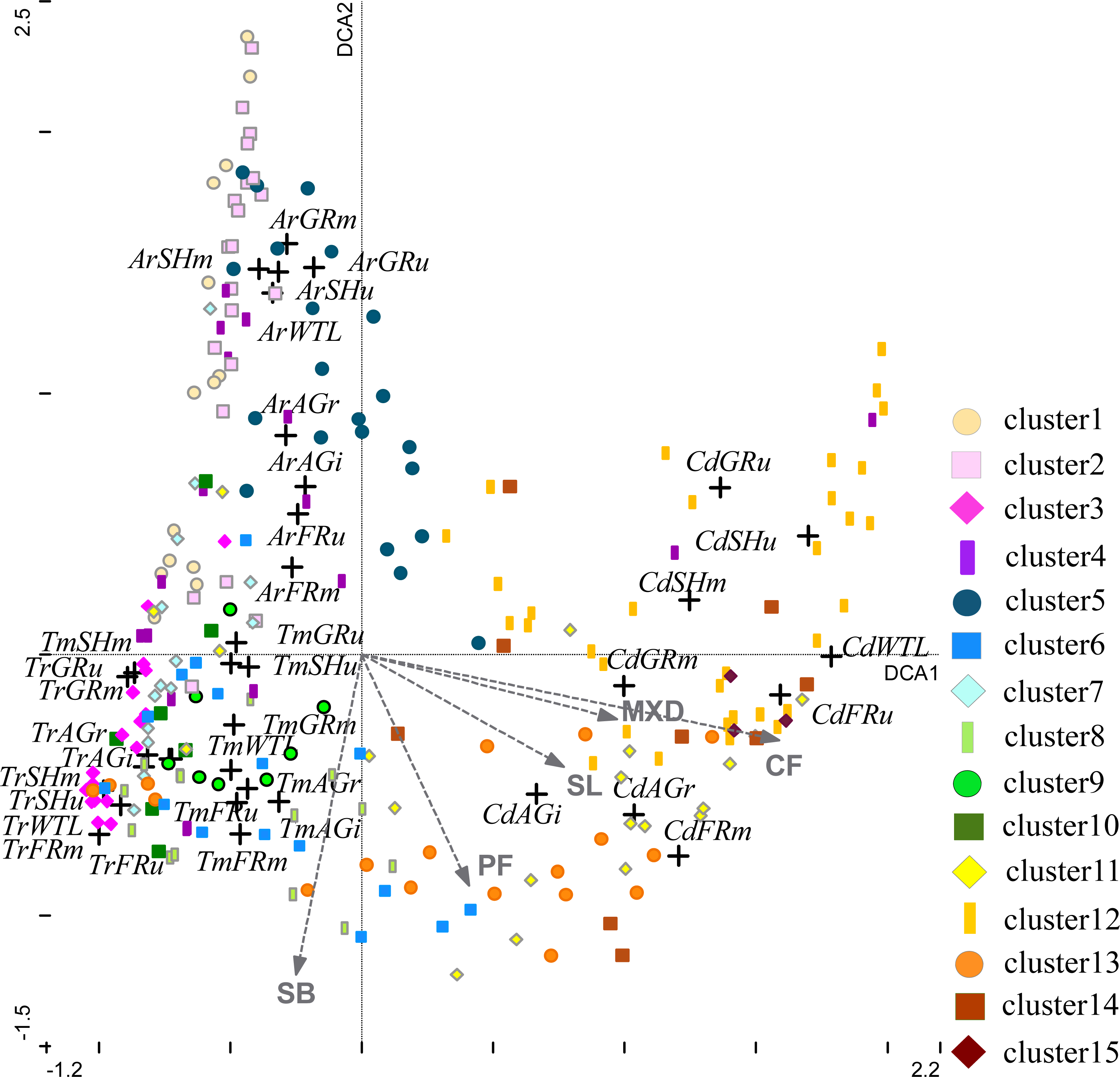
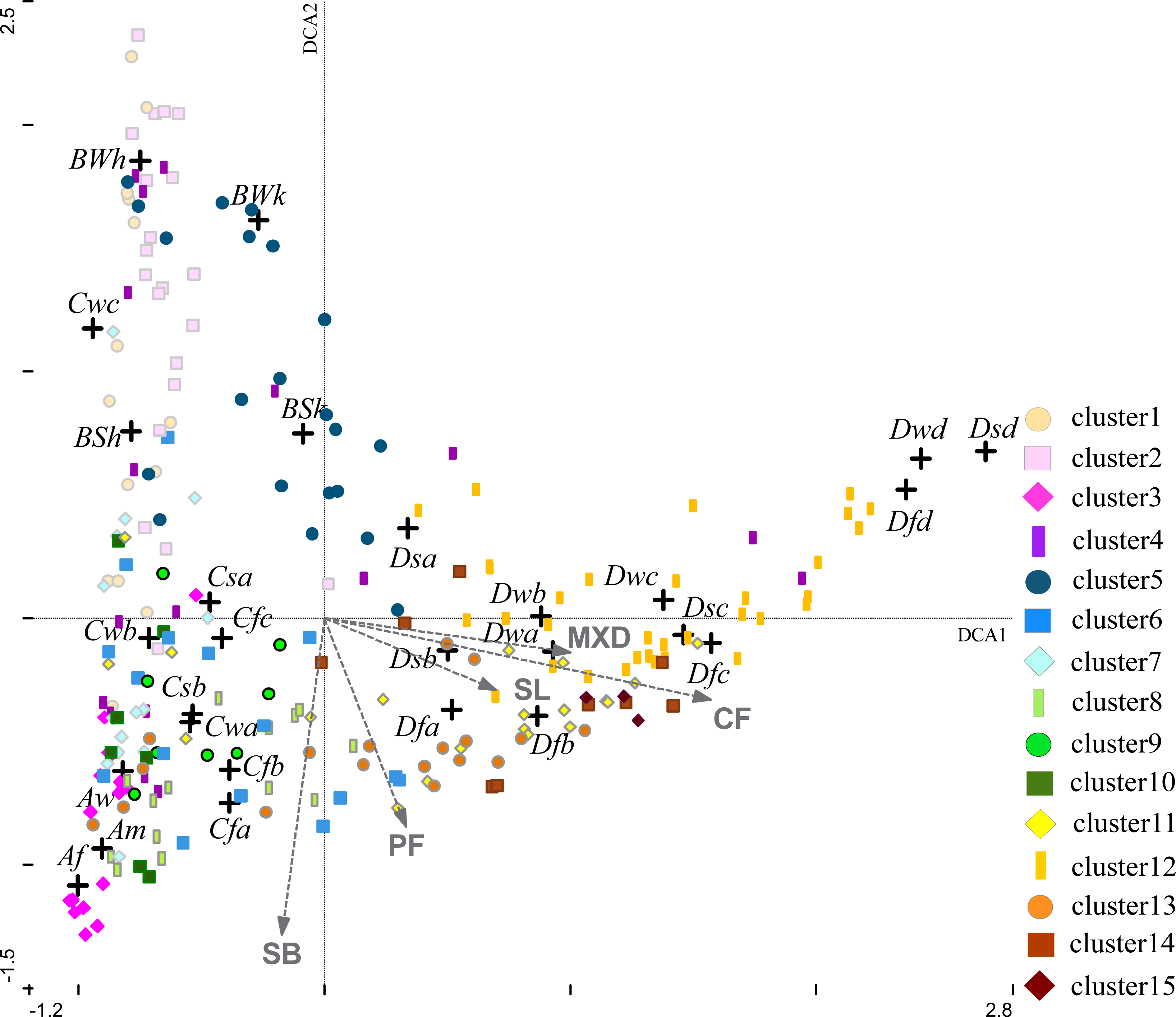
32]. A baseline characterization of ecosystem functioning is to be based on an up-to-date, effective and repeatable indicator system. Furthermore, regular updates are required as ecosystems rapidly change due to short time events such as droughts, floods, fires and human land use/intensification and longer term impacts due to climatic variability. Responsive and meaningful indicators are needed to assess the state and change of these ecosystems, including establishing causes and effects of degradation. With the aim to support monitoring of ecosystem functioning studies, we derived global EFTs from satellite measurements of seasonal vegetation dynamics. The EFTs showed a distinct spatial pattern in the PCA ordination but with overlap between the single categories conforming fuzzy boundaries of different ecosystems. Some overlap might also arise from the limits of remote sensing when observing seasonal vegetation dynamics over areas with low seasonality as e.g., over tropical areas or over areas with low vegetation cover. In fact, the tropical EFTs displayed strongly aggregated, thus less interpretable pattern when analyzing their correspondence with existing climate or with land use classifications. Nevertheless, the PCA ordination confirmed the potential of the EFTs in assessing the seasonal functioning of global ecosystems and the triplot enhanced the understanding of their phenological and productivity dynamics. Furthermore, it must be noted that droughts, floods, fires, land use intensification and longer term impacts due to climatic variability might change the functioning of the ecosystems. This is not reflected in the present study as we assessed EFTs based on the 30-year average functioning of the ecosystems. In order to assess changes in ecosystem dynamics, future studies should focus on yearly assessments and inter-annual variability of EFTs.
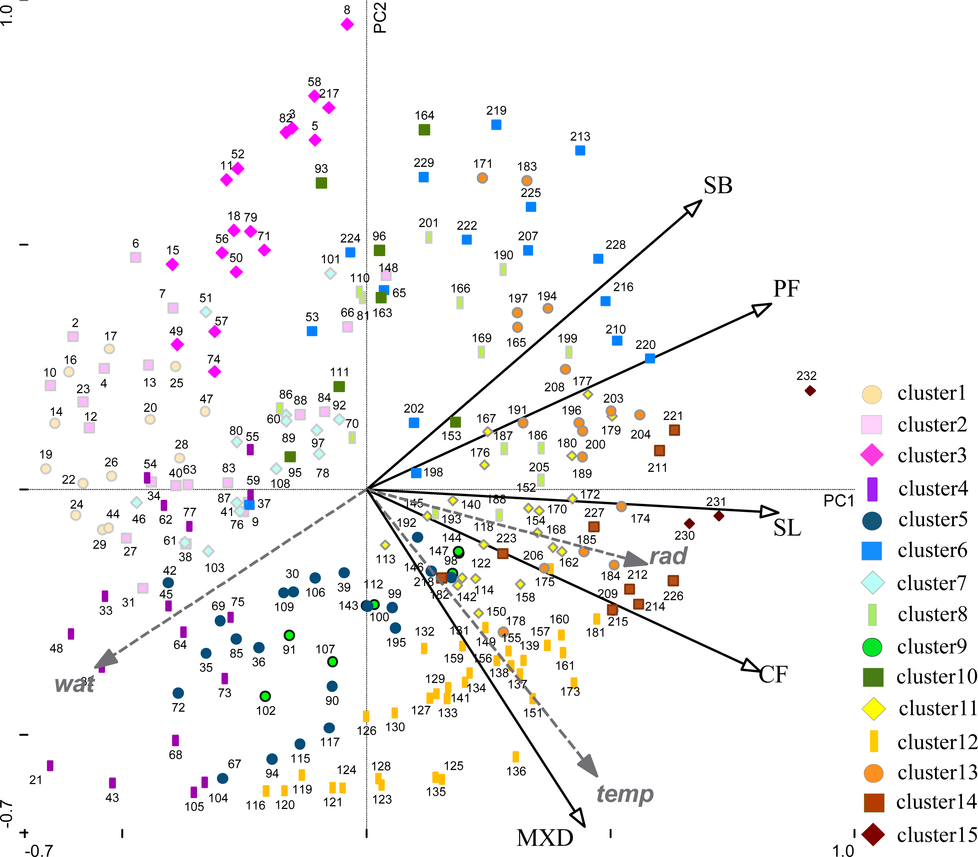
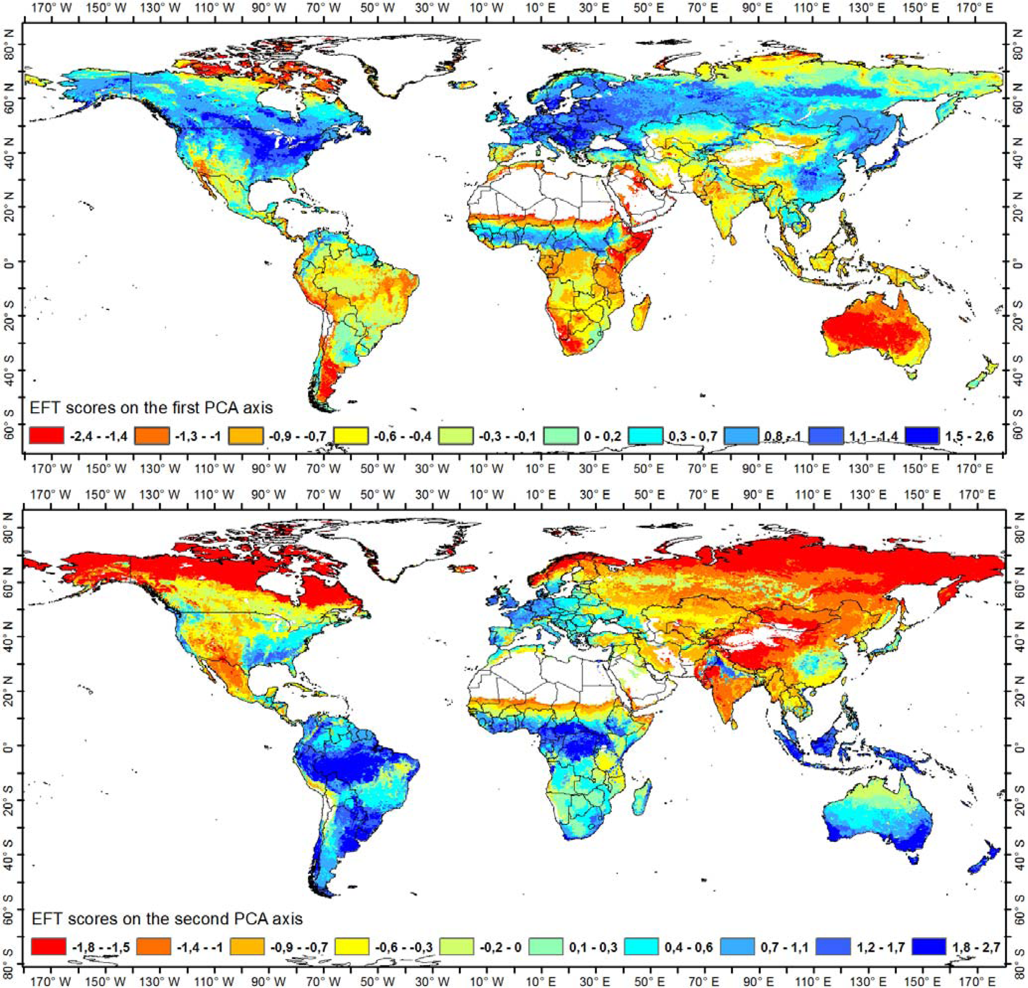
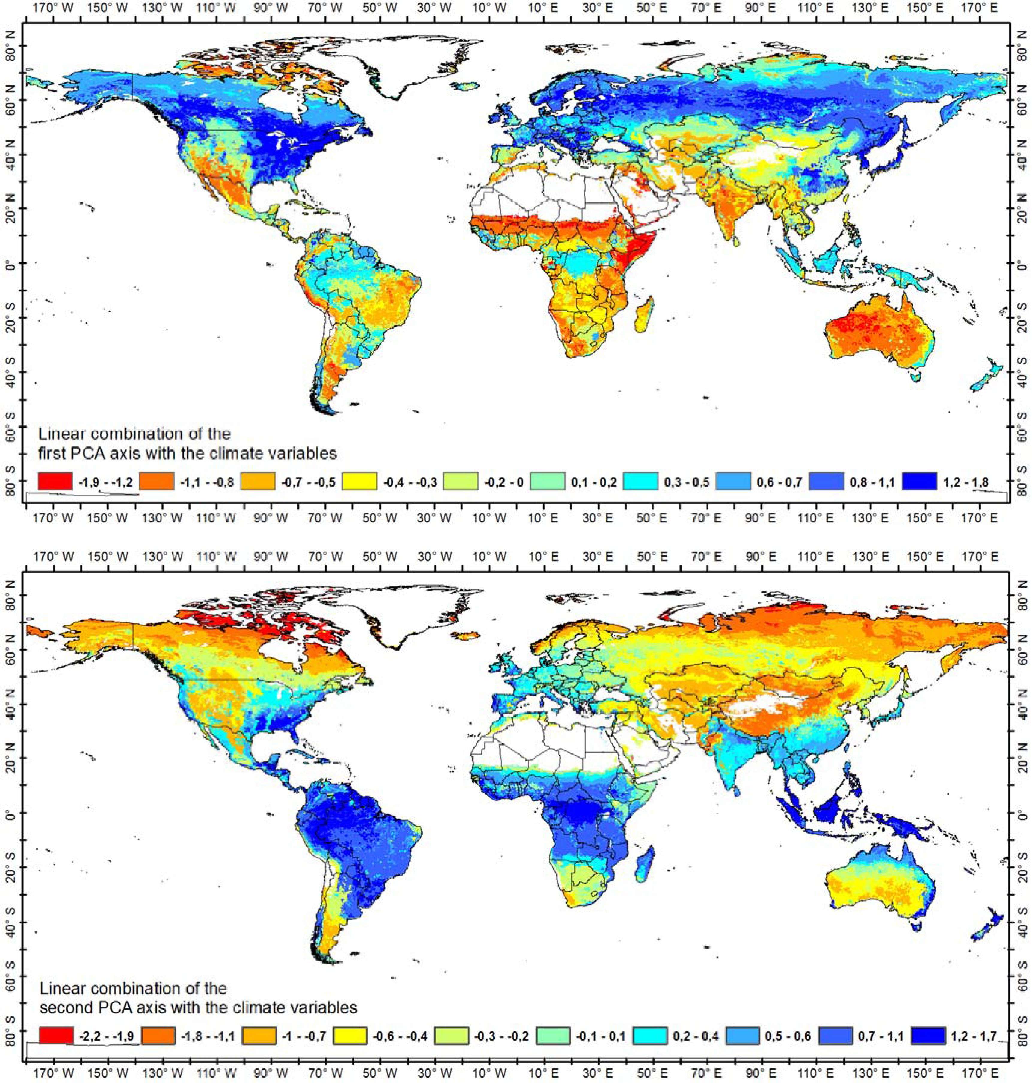
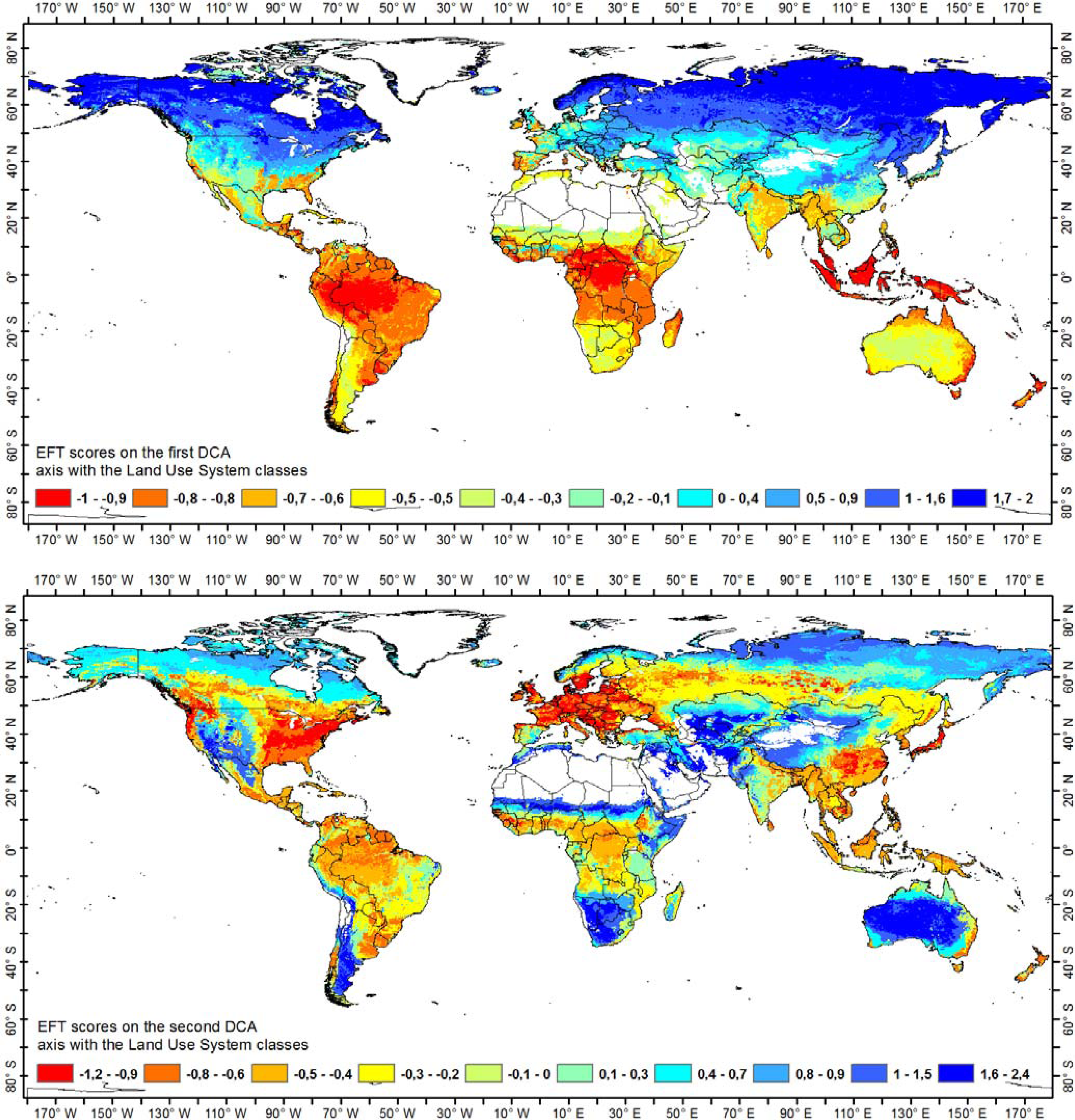
Climate is a main regional driver of ecosystem structure and functioning [52]. Therefore, to be valuable indicators of ecosystem functioning, the EFTs need to agree with climate gradients. The RDA indicated that the gradient of the EFTs and the phenology and productivity parameters along this gradient follow the global pattern of climatic vegetation growth constraints. The high percentage of variation explained by the first two axes in the gradient analysis showed that the EFTs captured two strong global environmental gradients. The first and stronger gradient positively related to water constraints and negatively related to radiation. The second, weaker gradient of the EFTs showed strongest correlation with the temperature growth constraint and moderate correlation to radiation constraints. For example, EFTs in high latitudes were shown to be controlled by temperature whereas EFTs in the arid and semi-arid areas were associated with water constraints of vegetation growth. We found a good correspondence of the global spatial pattern of these constraints within the EFTs and results of other authors on patterns of ecosystem-climate relationships (e.g., [29,32,44]). Nemani et al. [29] showed that water availability strongly limits vegetation growth over 40% of Earth’s vegetated surface, whereas temperature limits growth over 33% and radiation over 27%. Also Churkina and Running [44] showed that especially water but also temperature controls global NPP accumulation whereas radiation has considerably lower importance. Although we used a different variable for productivity than Churkina and Running [44], we obtained similar results showing that lowest productivity values were found in EFTs where water availability is the major climate constraint. We could further map a combined dependency of temperature and radiation using our extended set of variables. For instance, the yearly productivity expressed by the Cycling Fraction showed a strong association to temperature and radiation constraints for vegetation growth especially in the high latitudes. Furthermore, RDA suggested that the Maximum Day of the yearly vegetation signal is not related to water but rather to the constraining factor of temperature.
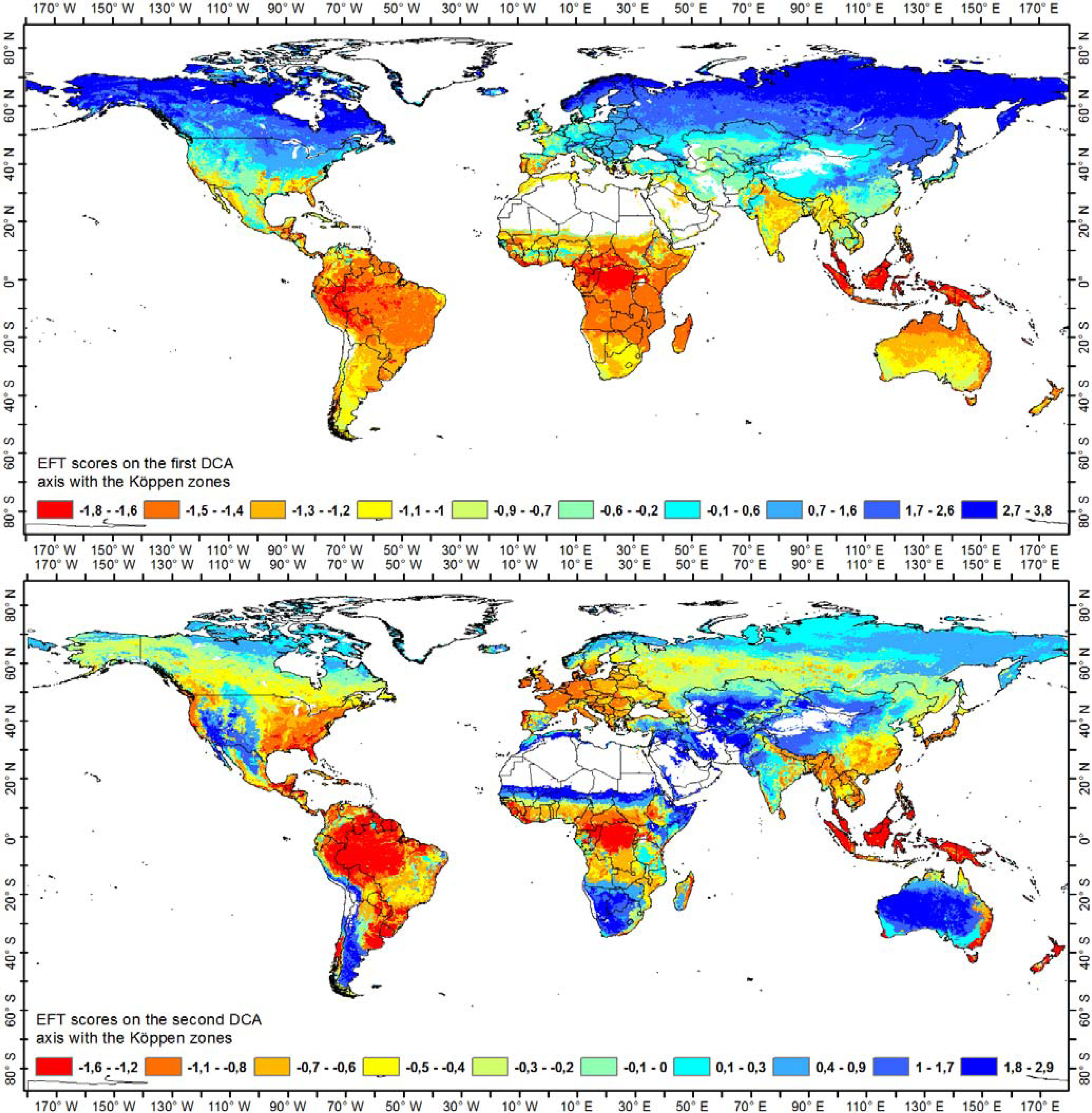
However, 50% of the variance in the global gradient of the EFTs could not be explained by the data indicating climatic constraints and variability and this should be attributed to other factors. On one hand, the climate and phenological data both have different time and spatial scales and associated noise/error that might play a role in the limited amount of explained variance. On the other hand, these results are consistent with Ivits et al. [
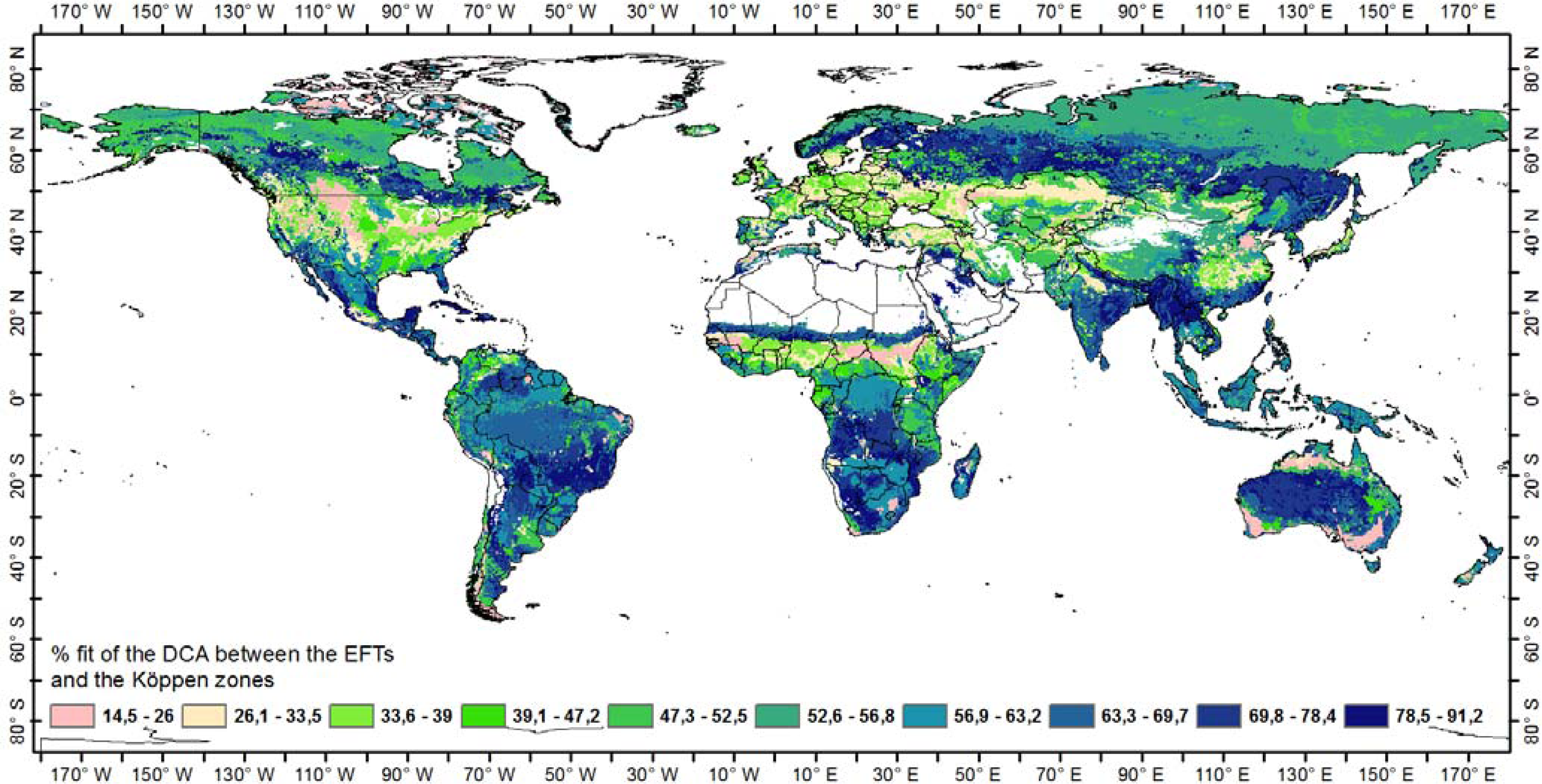
19] showing a limited temperature and precipitation dependency of the remote sensing derived phenological and productivity parameters for Europe. That it is not only climate controlling the distribution of EFTs is further supported by the correspondence analysis between the Köppen climate zones and the EFTs, which was 47%. Especially the cold and arid zones scored high, showing that over these regions vegetation phenology and productivity agrees with bio-climatic classification systems, which are mostly dependent on climatic constraints [19]. In other biomes, however, the correspondence was very low (low DCA fit) indicating that the Earth Observation derived variables comprise ecosystem functional information that is not inherent in bio-climatic classifications. Indeed, variations in vegetation signals are not only driven by climatic cycles but among others, by anthropogenic management practices [7]. This suggests that the functional types of global ecosystems might be substantially influenced by anthropogenic activities as well and that the EFTs, to be valuable indicators of ecosystem functioning, should also reflect differences in land use.
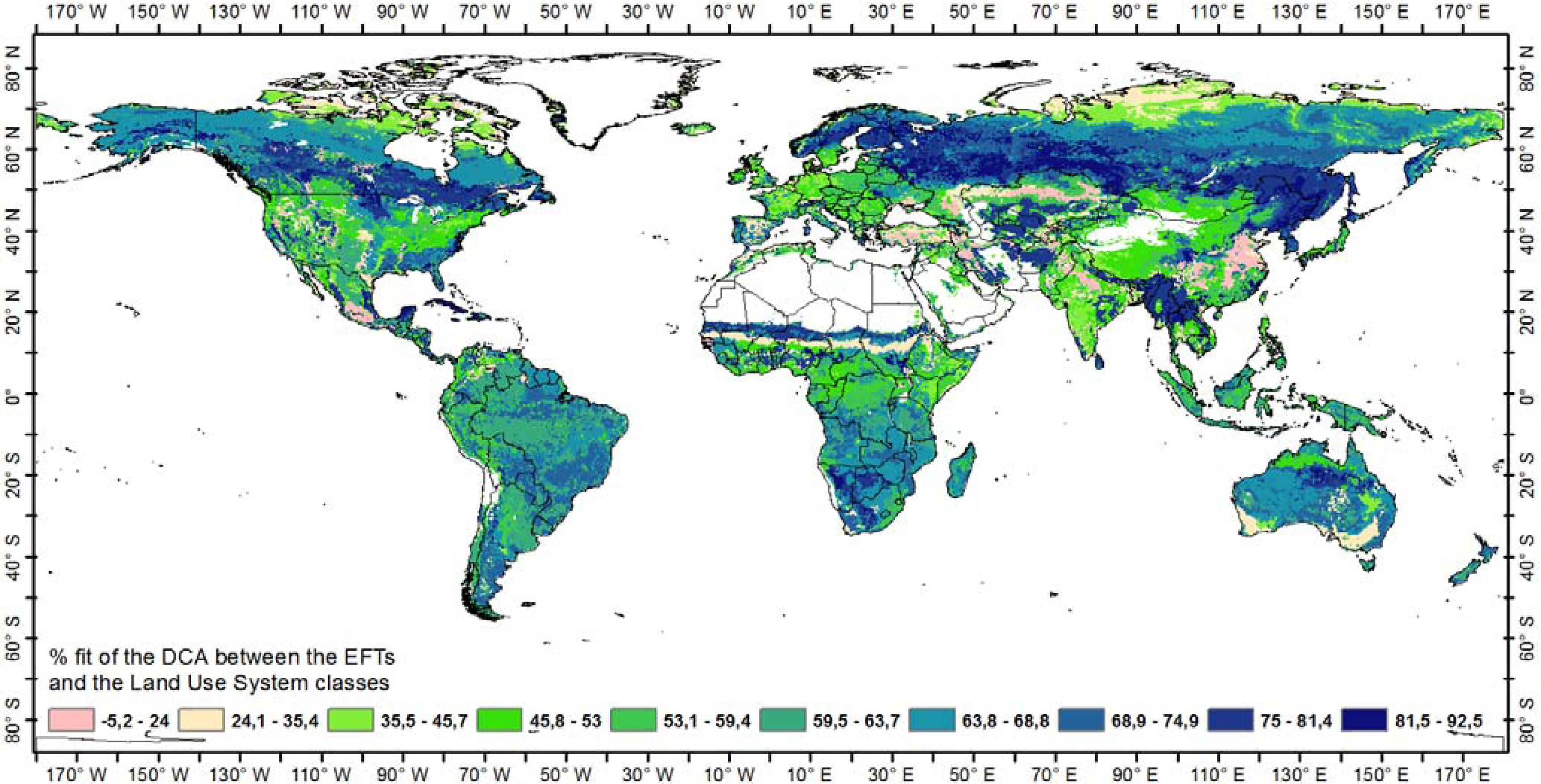
Differences in land use vary locally depending on the nature of the human pressure [32]. For example, harvest will characteristically cause earlier end of vegetation growing season and thus shorter season length as compared to natural areas. We therefore analyzed the relation between the EFTs and major global Land Use Systems testing how phenological and productivity parameters could enhance the understanding and characterization of these classifications. The influence of anthropogenic impacts on the EFTs was demonstrated by the 53.4% correspondence with the global Land Use Systems classes. Land use classes in the Cold and Arid zones were especially well discriminated by the EFTs whereas land use classes in the Tropical and Temperate zones, with more heterogeneous land use, were less interpretable. In a similar study, Ivits et al. [19] showed 85% correspondence of EFTs and European land covers using the 1km resolution SPOT VEGETATION data. In this global study based on the GIMMSs3g dataset, the results suggest that over more complex or intensively used areas the coarse spatial resolution of the remote sensing derived variables reach their limit in describing the spatial variability of vegetation cover. Hence, the response of EFTs to land use is dependent on the detail of spatial heterogeneity of the pixels potentially comprising all types of natural, semi-natural or intensively managed areas. Nevertheless, the present study demonstrated that EFTs do not only account for the climate dependence of ecosystem functioning but that they are also responsive to land use and thus supply indicators of the spatial patterns of ecosystem dynamics at larger spatial scales and offer an objective and repeatable method to characterise the functioning of ecosystems.

5. Conclusions

Using a time series of 30 years of Earth Observation derived phenological and productivity metrics, we stratified global ecosystems into Ecosystem Functional Types exhibiting similar patterns of seasonal phenology and productivity dynamics and similar responses to climate and land-use induced environmental conditions. The main findings of our analysis can be summarized as follows:
(1)
Gradient analysis confirmed the potential of the Ecosystem Functional Types in assessing the phenological and productivity dynamics of global ecosystems.
(2)
Redundancy Analysis showed that the gradient of the Ecosystem Functional Types indicates the global pattern of climatic vegetation growth constraints.
(3)
Correspondence Analysis confirmed that Ecosystem Functional Types relate to classification of global climatic zones.
(4)
Correspondence Analysis also indicated that it is not only climate controlling the distribution of Ecosystem Functional Types but that they also correspond to classifications of Land Use Systems, showing that the functional types of global ecosystems might be substantially influenced by anthropogenic activities as well.
(5)
By incorporating the spatial information of Earth Observation derived metrics into a new ecosystem functional map, we demonstrated that Ecosystem Functional Types comprise functional information that is not inherent in bio-climatic classifications and have potential in the monitoring of human influence on ecosystem functioning and in supporting ecosystem degradation studies.

Acknowledgments

The authors would like to thank the NASA Global Inventory Modelling and Mapping Studies (GIMMS) group for producing and sharing the GIMMS3g NDVI dataset. Thanks also to Ramakrishna Nemani for providing the potential climatic plant growth constraints data used in the analyses. This research was partly funded by the Danish Council for Independent Research (DFF) Sapere Aude programme under the project entitled “Earth Observation based Vegetation productivity and Land Degradation Trends in Global Drylands”.

Conflict of Interest

The authors declare no conflict of interest.

References

  1. Ayensu, E.; Claasen, D.V.; Collins, M.; Dearing, A.; Fresco, L.; Gadgil, M.; Gitay, H.; Glaser, G.; Lohn, C.L.; Krebs, J.; et al. Ecology—International ecosystem assessment. Science 1999, 286, 685–686. [Google Scholar]
  2. Ellis, E.C.; Ramankutty, N. Putting people in the map: Anthropogenic biomes of the world. Front. Ecol. Environ 2007, 6, 439–447. [Google Scholar]
  3. Lambin, E.F.; Geist, H.J. (Eds.) Land Use and Land Cover Change: Local Processes and Global Imoacts; Springer Verlag: New York, NY, USA, 2006; p. 222.
  4. Hellden, U.; Tottrup, C. Regional desertification: A global synthesis. Global Planet. Change 2008, 64, 169–176. [Google Scholar]
  5. Vogt, J.; Safriel, U.; von Maltitz, G.; Sokona, Y.; Zougmore, R.; Bastin, G.; Hill, J. Monitoring and assessment of land, Degradation and desertification—Towards new conceptual and integrated approaches. Land Degrad. Dev 2011, 22, 150–165. [Google Scholar]
  6. Fensholt, R.F.; Rasmussen, K.; Kaspersen, P.; Huber, S.; Horion, S.; Swinnen, E. Assessing land degradation/recovery in the African Sahel from long-term earth observation based primary productivity and precipitation relationships. Remote Sens 2013, 5, 664–686. [Google Scholar]
  7. Wessels, K.J.; Prince, S.D.; Malherbe, J.; Small, J.; Frost, P.E.; VanZyl, D. Can human-induced land degradation be distinguished from the effects of rainfall variability? A case study in South Africa. J. Arid Environ 2007, 68, 271–297. [Google Scholar]
  8. Prince, S.D. Mapping desertification in Southern Africa. In Land Change Science: Observing, Monitoring and Understanding Trajectories of Change on the Earth’s Surface; Gutman, G., Janetso, A., Eds.; Springer: Berlin, Germany, 2004; pp. 163–184. [Google Scholar]
  9. Walker, B.H. Biodiversity and ecological redundancy. Conserv. Biol 1992, 6, 18–23. [Google Scholar]
  10. Noble, I.R.; Gitay, H. A functional classification for predicting the dynamics of landscapes. J. Veg. Sci 1996, 7, 329–336. [Google Scholar]
  11. Diaz, S.; Abido, M. Plant functional types and ecosystem function in relation to global change. J. Veg. Sci 1997, 8, 463–474. [Google Scholar]
  12. Paruelo, J.M.; Jobbagy, E.G.; Sala, O.E. Current distribution of ecosystem functional types in temperate South America. Ecosystems 2001, 4, 683–698. [Google Scholar]
  13. Pennington, W. Lags in adjustment of vegetation to climate caused by the pace of soil development: evidence from Britain. Vegetatio 1986, 67, 105–118. [Google Scholar]
  14. Milchunas, D.G.; Laurenroth, W.K. Inertia in plant community structure: State changes after cessation of nutrient enrichment stress. Ecol. Appl 1995, 5, 1995–2005. [Google Scholar]
  15. McNaughton, S.; Oesterheld, M.; Frank, D.; Williams, K. Ecosystem-Level patterns of primary productivity and herbivory in terrestrial habitats. Nature 1989, 341, 142–144. [Google Scholar]
  16. Myneni, R.B.; Keeling, C.D.; Tucker, C.J.; Asrar, G.; Nemani, R.R. Increased plant growth in the northern high latitudes from 1981 to 1991. Nature 1997, 386, 698–702. [Google Scholar]
  17. Hill, J.; Stellmes, M.; Udelhoven, T.; Roder, A.; Sommer, S. Mediterranean desertification and land degradation: Mapping related land use change syndrimes based on satellite observations. Global Planet. Change 2008, 64, 146–157. [Google Scholar]
  18. Gu, Y.; Brown, J.F.; Miura, T.; van Leeuwen, W.J.D.; Reed, B.C. phenological classification of the United States: A geographic framework for extending multi-sensor time-series data. Remote Sens 2010, 2, 526–544. [Google Scholar]
  19. Ivits, E.; Cherlet, M.; Mehl, W.; Sommer, S. Ecosystem functional units characterized by satellite observed phenology and productivity gradients: A case study for Europe. Ecol. Indic 2013, 27, 17–28. [Google Scholar]
  20. McCloy, K.R. Development and evaluation of phenological change indices derived from time series of image data. Remote Sens 2010, 2, 2442–2473. [Google Scholar]
  21. Melendez-Pastor, I.; Navarro-Pedreño, J.; Koch, M.; Gómez, I.; Hernández, E.I. Land-Cover phenologies and their relation to climatic variables in an anthropogenically impacted Mediterranean coastal area. Remote Sens 2010, 2, 697–716. [Google Scholar]
  22. Motohka, T.; Nasahara, K.N.; Oguma, H.; Tsuchida, S. Applicability of green-red vegetation index for remote sensing of vegetation phenology. Remote Sens 2010, 2, 2369–2387. [Google Scholar]
  23. van Leeuwen, W.J.D.; Davison, J.E.; Casady, G.M.; Marsh, S.E. Phenological characterization of Desert Sky Island vegetation communities with remotely sensed and climate time series data. Remote Sens 2010, 2, 388–415. [Google Scholar]
  24. Kariyeva, J.; van Leeuwen, W.J.D. Environmental drivers of NDVI-based vegetation phenology in Central Asia. Remote Sens 2011, 3, 203–246. [Google Scholar]
  25. Ivits, E.; Cherlet, M.; Tóth, G.; Sommer, S.; Mehl, W.; Vogt, J.; Micale, F. Combining satellite derived phenology with climate data for climate change impact assessment. Global Planet. Change 2012, 88–89, 85–97. [Google Scholar]
  26. Chen, X.; Pan, W. Relationships among phenological growing season, time-integrated normalized difference vegetation index and climate forcing in the temperate region of eastern China. Int. J. Climatol 2002, 22, 1781–1792. [Google Scholar]
  27. Schwartz, M.D.; Reed, B.C. Surface phenology and satellite sensor-derived onset of greenness: An initial comparison. Int. J. Remote Sens 2002, 20, 3451–3457. [Google Scholar]
  28. Menzel, A. Trends in phenological phases in Europe between 1951 and 1996. Int. J. Biometeorol 2000, 44, 76–81. [Google Scholar]
  29. Nemani, R.R.; Keeling, C.D.; Hashimoto, H.; Jolly, W.M.; Piper, S.C.; Tucker, C.J.; Myneni, R.B.; Running, S.W. Climate-driven increases in global terrestrial net primary production from 1982 to 1999. Science 2003, 300, 1560–1563. [Google Scholar]
  30. Lloyd, D. A phenological classification of terrestrial vegetation cover using shortwave vegetation index imagery. Int. J. Remote Sens 1990, 11, 2269–2279. [Google Scholar]
  31. Soriano, A.; Paruelo, J.M. Biozones: Vegetation units defined by functional characters identifiable with the aid of satellite sensor images. Global Ecol. Biogeogr 1992, 2, 82–89. [Google Scholar]
  32. Alcaraz-Seguera, D.; Paruelo, J.M.; Epstein, H.E.; Cabello, J. Environmental and human controls of ecosystem functional diversity in temperate South America. Remote Sens 2013, 5, 127–154. [Google Scholar]
  33. Dregne, H.E. Land degradation in the drylands. Arid Land Res. Manag 2002, 16, 99–132. [Google Scholar]
  34. Stow, D.; Daeschner, S.; Boynton, W.; Hope, A. Arctic tundra functional types by classification of single-date and AVHRR bi-weekly NDVI composite datasets. Int. J. Remote Sens 2000, 21, 1773–1779. [Google Scholar]
  35. Alcaraz-Seguera, D.; Paruelo, J.M.; Cabello, J. Identification of current ecosystem functional types in the Iberian Peninsula. Global Ecol. Biogeogr 2006, 15, 200–212. [Google Scholar]
  36. Alcaraz-Seguera, D.; Cabello, J.; Paruelo, J. Basline characterisation of major Iberian vegetation types based on the NDVI dynamics. Plant Ecol 2009, 202, 13–29. [Google Scholar]
  37. Fernández, N.; Paruelo, J.M.; Delibes, M. Ecosystem functioning of protected and altered Mediterranean environments: A remote sensing classification in Doñana, Spain. Remote Sens. Environ 2010, 114, 211–220. [Google Scholar]
  38. Vermote, E.; Kaufman, Y.J. Absolute calibration of AVHRR visible and near-infrared channels using ocean and cloud views. Int. J. Remote Sens 1995, 16, 2317–2340. [Google Scholar]
  39. Los, S.O. Estimation of the ratio of sensor degradation between NOAA AVHRR channels 1 and 2 from monthly NDVI composites. IEEE Trans. Geosci. Remote Sens 1998, 36, 206–213. [Google Scholar]
  40. Stowe, L.L.; McClain, E.P.; Carey, R.; Pellegrino, P.; Gutman, G.G.; Davis, P.; Long, C.; Hart, S. Global distribution of cloud cover derived from NOAA/AVHRR operational satellite data. Adv. Space Res 1991, 3, 51–54. [Google Scholar]
  41. Tucker, C.J.; Pinzon, J.E.; Brown, M.E.; Slayback, D.A.; Pak, E.W.; Mahoney, R.; Vermote, E.F.; El Saleous, N. An extended AVHRR 8-km NDVI dataset compatible with MODIS and SPOT vegetation NDVI data. Int. J. Remote Sens 2005, 26, 4485–4498. [Google Scholar]
  42. Pinzon, J.E.; Brown, M.E.; Tucker, C.J. EMD Correction of Orbital Drift Artifacts in Satellite Datastream. In Hilbert-Huang Transform and Its Applications; Interdisciplinary Mathematical Sciences; Huang, N.E., Shen, S.P., Eds.; World Scientific: Singapore, 2005; Volume 5. [Google Scholar]
  43. Fensholt, R.; Proud, S.R. Evaluation of Earth observation based global long term vegetation trends—Comparing GIMMS and MODIS global NDVI time series. Remote Sens Environ 2012, 119, 131–147. [Google Scholar]
  44. Churkina, G.; Running, S.W. Contrasting climatic controls on the estimated productivity of global terrestrial biomes. Ecosystems 1998, 1, 206–215. [Google Scholar]
  45. Peel, M.C.; Finlayson, B.L.; McMahon, T.A. Updated world map of the Köppen-Geiger climate classification. Hydrol. Earth Syst. Sci 2007, 11, 1633–1644. [Google Scholar]
  46. Nachtergaele, F.; Petri, M. Land Degradation Assessment in Drylands: Mapping Land Use Systems at Global and Regional Scales for Land Degradation Assessment Analysis; Food and Agriculture Organization of the United Nations: Rome, Italy, 2011. [Google Scholar]
  47. Reed, B.; Brown, J.F.; Vanderzee, D.; Loveland, T.R.; Merchant, J.W.; Ohlen, D.O. Measuring phenological variability from satellite imagery. J. Veg. Sci 1994, 5, 703–714. [Google Scholar]
  48. Kaiser, H.F. The varimax criterion for analytic rotation in factor analysis. Psychometrika 1958. [Google Scholar] [CrossRef]
  49. Hill, M.O.; Gauch, H.G. Detrended correspondence analysis, an improved ordination technique. Vegetatio 1980, 42, 47–58. [Google Scholar]
  50. DeGaetano, A.T.; Knapp, W.W. Standardization of weekly growing degree day accumulations based on differences in temperature observation time and method. Agric. For. Meteorol 1993, 66, 1–19. [Google Scholar]
  51. Yang, S.; Logan, J.; Coffey, D.L. Mathematical formulae for calculating the base temperature for growing degree days. Agric. For. Meteorol 1995, 74, 61–74. [Google Scholar]
  52. Stephenson, N.L. Climatic control of vegetation distribution: The role of the water balance. Am. Nat 1990, 135, 649–670. [Google Scholar]
Figure 1. Schematic representation of the phenological and productivity variables calculated by Phenolo. Phenolo calculates all the areas under the time-series curve and all time and value of the depicted points on the yearly time-series curve. In the present study only the most important parameters were employed, which are listed on the right hand side.
Remotesensing 05 03305f1
Figure 2. Isodata classification of the spatial patterns of the first five rotated Principal Components (top). The iterative classification resulted in 232 Ecosystem Functional Types (EFTs). By minimizing variance within the classes the EFTs were regrouped into 15 major clusters (bottom). White areas represent pixels without vegetation cover.
Remotesensing 05 03305f2
Figure 3. Ordination triplot of the gradient PCA analysis. The icons represent the 232 EFTs (numbers) classified into 15 clusters (icons). Full arrows represent the Phenolo variables (see Figure 1) whereas dashed arrows show climatic constraints of vegetation growth (wat = water, temp = temperature, rad = radiation). The horizontal axis shows the first PCA axis (55.9% variation explained) whereas the vertical axis shows the second axes (23.2% variation explained).
Remotesensing 05 03305f3
Figure 4. Spatial patterns of the first (top) and second (bottom) axis of the gradient PCA ordination of the selected Phenolo variables averaged within the EFT clusters. White areas represent pixels without vegetation cover.
Remotesensing 05 03305f4
Figure 5. Linear combination of the first (top) and second (bottom) gradient PCA axes with the variables indicating climatic constraints of vegetation growth. White areas represent pixels without vegetation cover.
Remotesensing 05 03305f5
Figure 6. Detrended Correspondence Analysis (DCA) triplot of the EFTs classified in 15 clusters (icons with colors) and the Köppen climate zones (crosses). Arrows represent the phenological and productivity variables averaged within the EFTs. Their positions indicate the correlation with the DCA axes.
Remotesensing 05 03305f6
Figure 7. Spatial patterns of the first (top) and second (bottom) axis derived from DCA of the EFTs with the Köppen zones. White areas represent pixels without vegetation cover.
Remotesensing 05 03305f7
Figure 8. Percentage fit for the DCA of the EFTs with the Köppen zones. High values indicate good fit of the two datasets. White areas represent pixels without vegetation cover.
Remotesensing 05 03305f8
Figure 9. DCA triplot of the EFTs classified in 15 clusters (icons with colors) and the Land Use System classes (crosses). Arrows represent the phenological and productivity variables averaged within the EFTs. Their position indicates the correlation with the DCA axes.
Remotesensing 05 03305f9
Figure 10. Spatial patterns of the first (top) and second (bottom) axis derived from DCA of the EFTs with the Land Use System classes. White areas represent pixels without vegetation cover.
Remotesensing 05 03305f10
Figure 11. Percentage fit for the DCA of the EFTs with the land Use System classes. High values indicate good fit of the two datasets. White areas represent pixels without vegetation cover.
Remotesensing 05 03305f11
Table 1. Köppen climatic zones and FAO Land Use Systems classes used in the present study.
LUS ClassesCodeKöppen Climatic ZonesCodeKöppen Climatic ZonesCode
Forests, unmanagedFRuTropical rainforestAfTemperate, dry winter, cold summerCwc
Forests, managedFRmTropical MonsoonAmCold, dry and hot summerDsa
Grassland, unmanagedGRuTropical SavannahAwCold, dry and warm summerDsb
Grassland, managedGRmArid, desert, hotBwhCold, dry and cold summerDsc
Shrubland, unmanagedSHuArid, desert, coldBwkCold, dry summer, very cold winterDsd
Shrubland, managedSHmArid, steppe, hotBshCold, dry winter, hot summerDwa
Rainfed agricultureAGrArid, steppe, coldBskCold, dry winter, warm summerDwb
Irrigated agricultureAGiTemperate, Dry and hot summerCsaCold, dry winter, cold summerDwc
WetlandsWTLTemperate, Dry and warm summerCsbCold, dry and very cold winterDwd
Temperate, no dry season, hot summerCfaCold, no dry season, hot summerDfa
Temperate, no dry season, warm summerCfbCold, no dry season, warm summerDfb
Temperate, no dry season, cold summerCfcCold, no dry season, cold summerDfc
Temperate, dry winter, hot summerCwaCold, no dry season, very cold winterDfd
Temperate, dry winter, warm summerCwb
Table 2. Principal Component Analysis (PCA) of the phenological and productivity variables. Statistics for the first five varimax rotated components are shown.
ComponentEigenvalues% of Explained VarianceCumulative % of Explained Variance
Screening PCA with 10 variables (as in Figure 1)

14.141.141.1
21.919.460.5
31.717.477.9
41.312.590.4
50.88.298.6

Final PCA with 5 selected variables

11.0621.221.2
21.0220.441.6
31.0120.361.9
40.9919.981.8
50.9118.2100.0
Table 3. Normalized loadings of the selected phenological variables on the first five rotated axes of the final PCA.
Rotated PCA Components

VariablesPC1PC2PC3PC4PC5
Season Length0.1840.9280.0860.1990.239
Permanent Fraction0.3920.289−0.0160.1480.861
Cyclic Fraction0.0320.1930.2650.9360.122
Standing Biomass0.9280.178−0.1040.0240.308
Maximum Day−0.0930.0740.9630.242−0.016
Table 4. Redundancy Analysis (RDA) of the phenological and productivity variables averaged within the EFTs as dependent variables and the climatic constraints averaged within the EFTs as explanatory variables.
Axis1Axis2Axis3Axis4
Eigenvalues0.3430.1390.0180.226
Cumulative % of explained variance34.348.350.072.7
Sum of canonical eigenvalues0.500
Monte Carlo test: F-ratio/significance76.135/p < 0.001
Table 5. Detrended Correspondence Analysis (DCA) of the EFTs with the Köppen climate zones.
Axis1Axis2Axis3Axis4
Eigenvalues0.6410.3540.1570.065
Cumulative % of explained variance30.146.754.157.1
Table 6. DCA of the EFTs with the Land Use System classes.
Axis1Axis2Axis3Axis4
Eigenvalues0.5860.3060.0770.043
Cumulative % of explained variance35.153.458.060.6

