Super-Resolution Reconstruction for Multi-Angle Remote Sensing Images Considering Resolution Differences

Abstract

Multi-angle remote sensing images are acquired over the same imaging scene from different angles, and share similar but not identical information. It is therefore possible to enhance the spatial resolution of the multi-angle remote sensing images by the super-resolution reconstruction technique. However, different sensor shooting angles lead to different resolutions for each angle image, which affects the effectiveness of the super-resolution reconstruction of the multi-angle images. In view of this, we propose utilizing adaptive weighted super-resolution reconstruction to alleviate the limitations of the different resolutions. This paper employs two adaptive weighting themes. The first approach uses the angle between the imaging angle of the current image and that of the nadir image. The second is closely related to the residual error of each low-resolution angle image. The experimental results confirm the feasibility of the proposed method and demonstrate the effectiveness of the proposed adaptive weighted super-resolution approach.

1. Introduction

High-resolution remote sensing satellite imagery provides rich, detailed information and allows high-definition visual interpretation. High-resolution images can therefore support improved information extraction capabilities at a fine scale. Nowadays, high-resolution (HR) images are widely used for land surveys, urban studies, forest measurement, hazard assessment, military target identification, and so on. In order to improve the spatial resolution of the observed images, the traditional method is to decrease the physical sizes of the charge-coupled device (CCD) or complementary metal oxide semiconductor (CMOS) sensors through advanced sensor fabrication techniques, which is referred to as the hardware approach. However, this generates shot noise that severely degrades the image quality. There is therefore a technical limitation with regard to pixel size reduction [1,2]. In addition, the economic cost of manufacturing such high-precision equipment is very high. Thus, it is necessary to develop post-processing software techniques to improve the spatial resolution of remote sensing images, and the super-resolution reconstruction (SRR) technique has become widely acknowledged as an efficient approach for remote sensing image resolution enhancement.

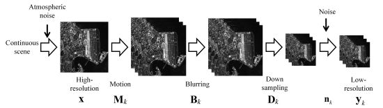
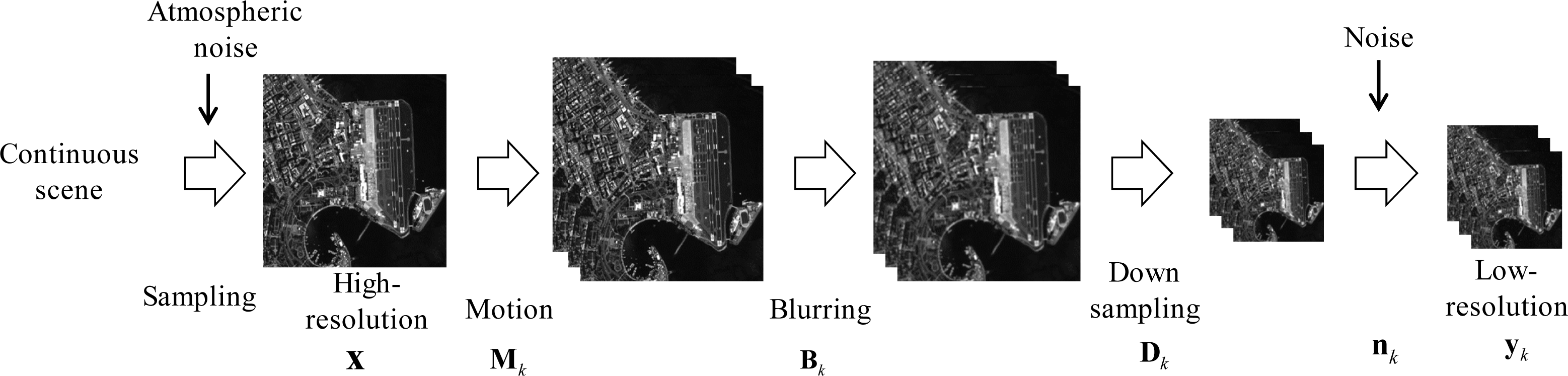
Image super-resolution reconstruction refers to a signal processing technique which produces a high-resolution image from a sequence of observed low-resolution (LR) images that are noisy, blurred, and downsampled [3,4]. The idea of SRR was first proposed in 1984 by Tsai and Huang [5] to improve the spatial resolution of Landsat TM images, using multiple under-sampled images with sub-pixel displacements in the frequency domain. Since then, the super-resolution reconstruction technique has developed greatly, and there have been various classical reconstruction frameworks proposed, such as the maximum a posteriori (MAP) [6], projection onto convex sets (POCS) [7], non-uniform interpolation [8], maximum likelihood [9,10], the iterative back-projection approach (IBP) [11], mixed maximum a posteriori/projection onto convex sets (MAP/POCS) [12], and so on. Generally speaking, the SRR methods in the frequency domain have a fast processing speed, but it is usually difficult to integrate the prior knowledge of the reconstruction image. Therefore, the spatial domain methods have been more widely used, due to their flexible image and noise modeling capabilities.

As previously mentioned, the earliest idea for super-resolution reconstruction came from remote sensing image resolution enhancement. To date, the most successful application of super-resolution reconstruction in remote sensing is the SPOT-5 satellite system. This system shifts half a sampling interval in the horizontal and vertical directions by a double CCD linear array, which obtains two panchromatic 5 m resolution images, and then produces an approximately 2.5 m resolution high-resolution image through super-resolution reconstruction processing [13]. This is a successful example of the application of super-resolution reconstruction in remote sensing via the combination of the hardware approach and the post-processing software approach. In recent years, the super-resolution reconstruction of remote sensing images has mainly focused on multi-temporal image sequences. Merino et al. [14] proposed a variable-pixel linear reconstruction based super-resolution reconstruction algorithm and conducted experiments with Landsat ETM+ images. Shen et al. [15] proposed a super-resolution reconstruction algorithm for use with Moderate Resolution Imaging Spectroradiometer (MODIS) images. Li et al. [16] proposed a method based on a universal hidden Markov tree model for remote sensing images and tested it with Landsat7 panchromatic images captured on different dates. The imaging interval of multi-temporal satellite images over the same scene may, however, be several days or even much longer. Between the adjacent imaging moments, the imaging scene or weather conditions may change, which poses great difficulties for the super-resolution reconstruction of multi-temporal remote sensing images.

The multi-angle remote sensing imaging system obtains images at different angles within a very short time span, such that the imaging scene and weather conditions hardly change at all. The multi-angle images of the same scene contain sub-pixel displacements, so they are more suitable for super-resolution reconstruction than a multi-temporal image sequence. Therefore, scholars have recently begun to utilize multi-angle remote sensing images for super-resolution reconstruction. Chan et al. [17] proposed registering multi-angle CHRIS/Proba images with a thin-plate spline non-rigid transform model and conducted super-resolution reconstruction experiments with Delaunay triangulation based non-uniform interpolation. Ma et al. [18] proposed an operational SR approach for multi-angle WorldView-2 remote sensing images, which consists of two stages: image registration and super-resolution reconstruction. Image registration accounts for the local geometric distortion and photometric disparity. The SRR model is composed of an L1 norm data fidelity item and total variation (TV) regularization. 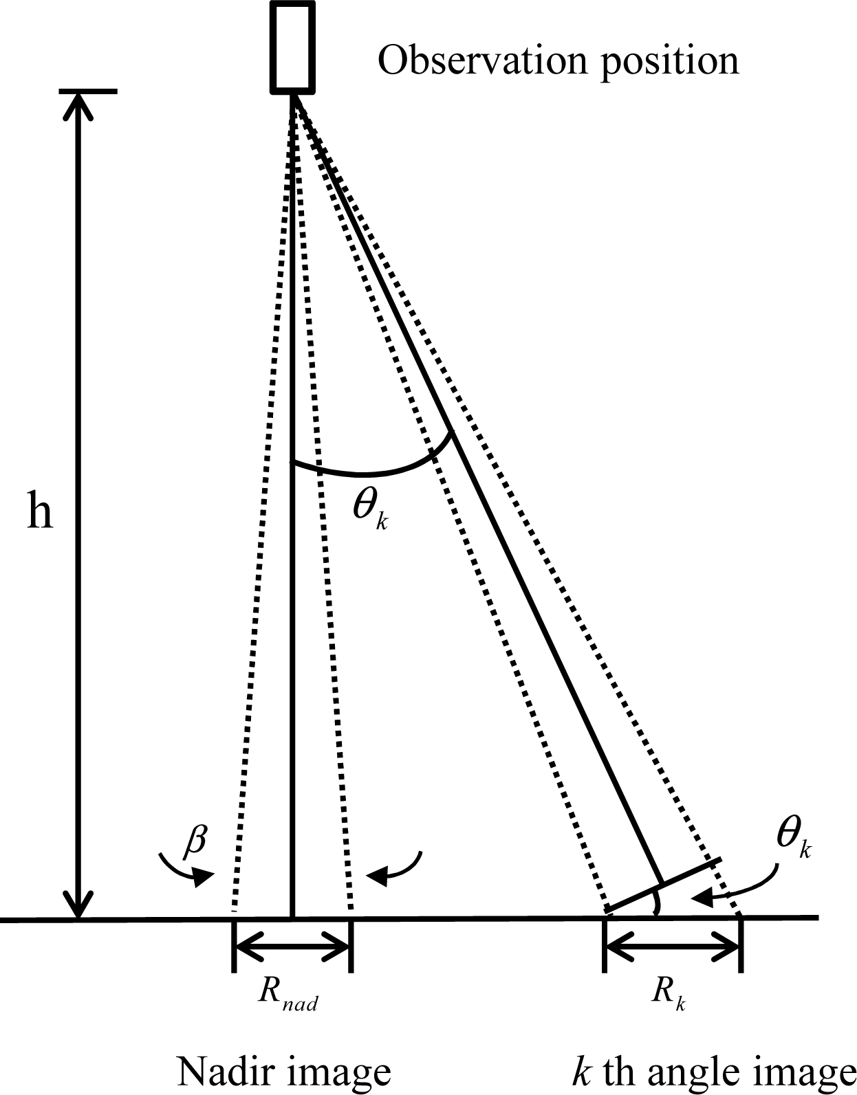Galbraith et al. [19] noted that the spatial resolution of different angle images is different, and the spatial resolution of an off-nadir image will be lower than that of the nadir image. Hence, the contributions of different angle images to the reconstructed image will be different.

In view of this, we propose an adaptive weighted super-resolution reconstruction algorithm considering the different resolutions of multi-angle remote sensing images. The different contributions of the multi-angle LR images, which arise from their different resolutions, are reflected by different weights. Two different weighting schemes are utilized in this paper. The first scheme uses the relative angle between the imaging angle of the current image and that of the nadir image. The second is closely related to the residual error of each low-resolution angle image. The proposed model consists of a data fidelity item based on an ℓ₂ norm and the TV model as the regularization item. The extensive experimental results confirm the feasibility and superiority of our proposed method.

The structure of the paper is as follows. In Section II, we introduce the general super-resolution model and describe the proposed adaptive weighted SRR approach in detail. We then give the experiments and the experimental analysis in Section III. Finally, we conclude the paper and discuss the directions of our future work in Section IV.

2. The Adaptive Weighted Super-Resolution Reconstruction Method for Multi-Angle Images

2.1. Observation Model

An image super-resolution observation model is used to simulate the imaging degradation process of the remote sensing sensor imaging system. The input is a continuous natural scene, in which the scene signals are contaminated by the atmospheric noise before reaching the image system, and then sampled according to the Nyquist sampling theorem, to obtain the HR images. Through the sensor capturing process, multi-frame low-resolution remote sensing images are generated over the same scene into the camera sensor area [20]. In the imaging process, the obtained low-resolution images suffer from various degradation issues, including motion effects, blurring, noise, and downsampling. The motion effects usually include rotation and shift. The blurring effects comprise optical blurring and motion blurring.

Let x be the high-resolution image to be constructed, and y_k denotes the k-th low-resolution angle image. D_k is the k-th downsampling operator. B_k represents the blurring effects. M_k expresses the motion displacement information between the reference image and the k-th angle image. n_k represents the noise. We can then obtain the observation model:

$${\mathbf{y}}_k={\mathbf{D}}_k{\mathbf{B}}_k{\mathbf{M}}_k\mathbf{x}+{\mathbf{n}}_k\hspace{0.17em}\hspace{0.17em}k=1,2,\dots ,Z$$

1

where the size of the LR image is m, n in the horizontal and vertical directions, and the resolution enhancement factor between the HR image and LR image is set as r. Z is the total number of multi-angle images. y_k and n_k are both of the size mn × 1. Matrices B_k and M_k have the same size of r²mn × r² mn. The size of D_k is mn × r² mn. x represents the original HR image with the size of r²mn × 1. It is assumed that the downsampling matrix D_k and the blurring matrix B_k are both the same for all the LR images, and are denoted as D and B, respectively. The graphical simulation imaging process for acquiring the digital images is shown in Figure 1. In the practical experiments, the three matrices D, B and M_k are constructed with the resolution enhancement factor, blurring kernel function and image motion shift, respectively.

2.2. The Adaptive Weighted Super-Resolution Reconstruction Method

The super-resolution reconstruction is an inverse process of the imaging process, and is usually considered as an ill-posed inverse problem. In order to obtain a more desirable result, a regularization method is utilized to stabilize the ill-posed inverse problem. Traditionally, regularization can be described from both the algebraic and statistical perspectives [4]. Using regularization techniques, the desired HR image can be obtained by solving the following cost function:

$$\widehat{\mathbf{x}}=\mathit{arg}\hspace{0.17em}\text{min}\left[\sum _{k=1}^Z\rho ({\mathbf{y}}_k-{\mathbf{DBM}}_k\mathbf{x})+\lambda U(\mathbf{x})\right]$$

(2)

where ρ(y_k−DBM_kx) and U(x) are referred to as the data fidelity item and the regularization item, respectively. λ is the regularization parameter that controls the relative contribution between them.

The data fidelity item ρ(y_k−DBM_kx) provides a measure of the conformance of the estimated image to the observed image, according to the image observation model [2]. It is determined by the type of the noise vector n_k in Equation (1). Assuming that the noise is additive white Gaussian noise (AWGN), the data fidelity item can be given by:

$$\rho ({\mathbf{y}}_k-{\mathbf{DBM}}_k\mathbf{x})={\Vert {\mathbf{y}}_k-{\mathbf{DBM}}_k\mathbf{x}\Vert }^2$$

3

The regularization item U(x) imposes the spatial constraints on the image. The TV regularization model [22–23] is utilized here to regularize the ill-posed problem, and can be expressed as:

$$U(\mathbf{x})={\Upsilon }_{\mathit{TV}}(\mathbf{x})=\sum _i\sum _j\sqrt{{\Vert \nabla {\mathbf{x}}_i\Vert }^2+{\Vert \nabla {\mathbf{x}}_j\Vert }^2+\mu }$$

(4)

where ▿x_i = x[i+1, j] − x[i, j] and ▿x_j = x[i, j+1] − x[i, j]. i and j represent the image position in the horizontal and vertical directions, respectively, and μ is a small positive parameter which ensures differentiability of the model. It is set to 0.01 in this paper. Substituting Equations (3) and (4) into Equation (2), we can get the following minimization cost function:

$$\widehat{\mathbf{x}}=\mathit{arg}\hspace{0.17em}\text{min}\left[\sum _{k=1}^Z{\Vert {\mathbf{y}}_k-{\mathbf{DBM}}_k\mathbf{x}\Vert }^2+\lambda {\Upsilon }_{\mathit{TV}}(\mathbf{x})\right]$$

(5)

In the multi-angle remote sensing image SRR case, the spatial resolution of the different angle images is different. Consequently, the amount of information that the desired reconstruction image obtains from each different angle image is also different. Therefore, there is a requirement for us to discriminate their different contributions and treat them unequally in the super-resolution process. In this paper, we propose utilizing a weighted super-resolution reconstruction energy function model, as shown in Equation (6):

$$\widehat{\mathbf{x}}=\mathit{arg}\hspace{0.17em}\text{min}\left[\sum _{k=1}^Z{W}_k{\Vert {\mathbf{y}}_k-{\mathbf{DBM}}_k\mathbf{x}\Vert }^2+\lambda {\Upsilon }_{\mathit{TV}}(\mathbf{x})\right]$$

(6)

where W_k is the weight value for the k-th angle image. The two adaptive weighting schemes are introduced in the next subsection.

As the TV model shown in Equation (4) is nonlinear with respect to x, the lagged diffusivity fixed-point iteration [24] is utilized here. We then use the steepest descent method to solve the weighted super-resolution reconstruction model:

$${\widehat{\mathbf{x}}}_{n+1}={\widehat{\mathbf{x}}}_n+\alpha \left\{\sum _{k=1}^Z{W}_k\hspace{0.17em}{\mathbf{M}}_k^T\hspace{0.17em}{\mathbf{B}}^T\hspace{0.17em}{\mathbf{D}}^T({\mathbf{y}}_k-{\mathbf{DBM}}_k\hspace{0.17em}{\widehat{\mathbf{x}}}_n)-\lambda {\Gamma }_{\mathit{TV}}({\widehat{\mathbf{x}}}_n)\right\}$$

(7)

where α is a scalar defining the step size in the reverse direction of the gradient. x̂_n is the reconstruction result for the n-th iteration, and the initial value takes the bilinear interpolation of the reference LR image. Γ_TV(x) is the partial derivative of the TV regularization model ϒ_TV(x) with respect to x.

2.3. Adaptive Weighting Methods

This subsection introduces the two adaptive weighting schemes. The first method assigns the weight for each angle image by the angle difference between its imaging angle and that of the nadir image. The other method builds a connection between the weight for each angle image and its corresponding residual, according to the image observation model. Generally speaking, the image which is the closest to the nadir image is selected as the reference image and should be assigned the largest weight value.

2.3.1. The Angular Difference Weighting Method

An illustration of a multi-angle imaging system is shown in Figure 2 [19].

In Figure 2, β represents the instantaneous field of view angle. θ_k is the relative angle between the nadir image and the k-th angle image. h is the height from the sensor to the ground. R_nad represents the spatial resolution of the nadir image, and R_k denotes that of the k-th angle image. Through a series of deductions [19], the relationship between the spatial resolution of the two images can be expressed as:

$$R_k=\frac{\beta h}{{\text{cos}}^2\hspace{0.17em}{\theta }_k}=\frac{R_{\mathit{nad}}}{{\text{cos}}^2\hspace{0.17em}{\theta }_k}$$

(8)

It is observed that the spatial resolution of the nadir image is the highest, and the larger the imaging angle of the k-th angle image, the smaller its spatial resolution is. It is natural that the nadir image should be assigned the largest weighted value, and the weighted values of the other angle images should be decreased with the increase of the relative angle between the nadir image and the k-th angle image. Therefore, following the relationship between the spatial resolutions of the two images, we build the following weighting function:

$$W_k={\text{cos}}^2\hspace{0.17em}{\theta }_k$$

(9)

where W_k represents the weight for the k-th angle image, and θ_k is the relative angle between the k-th angle image and the nadir image.

2.3.2. Residual Weighting Method

The other weighting approach is closely related to the residual errors. As already mentioned, the image which is the closest to the nadir image is selected as the reference image, which has the highest spatial resolution among all the multi-angle images, so the residual error of an image with a low resolution will obviously be large. Therefore, the weights can be set as inversely proportional to the residual error of each different angle image. Here, to alleviate the resolution difference problem, we utilize the weighting method which was originally proposed by Hu et al. [25] to handle the different levels of registration errors of LR images. The weight value for the k-th angle image can be expressed as:

$$W_k=\frac{C}{{\Vert {\mathbf{y}}_k-{\mathbf{DBM}}_k\mathbf{x}\Vert }^2}$$

(10)

where ‖y_k−DBM_kx‖² is the residual term for the k-th angle image, and C is defined as:

$$C=\frac{Z}{\sum _{k=1}^Z\frac{1}{{\Vert {\mathbf{y}}_k-{\mathbf{DBM}}_k\mathbf{x}\Vert }^2}}$$

(11)

3. Experimental Section

3.1. Experimental Data and Setup

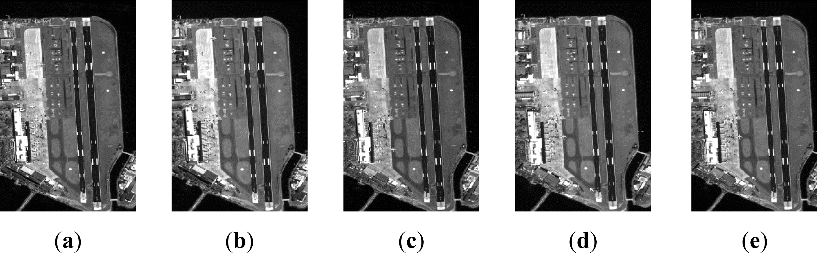
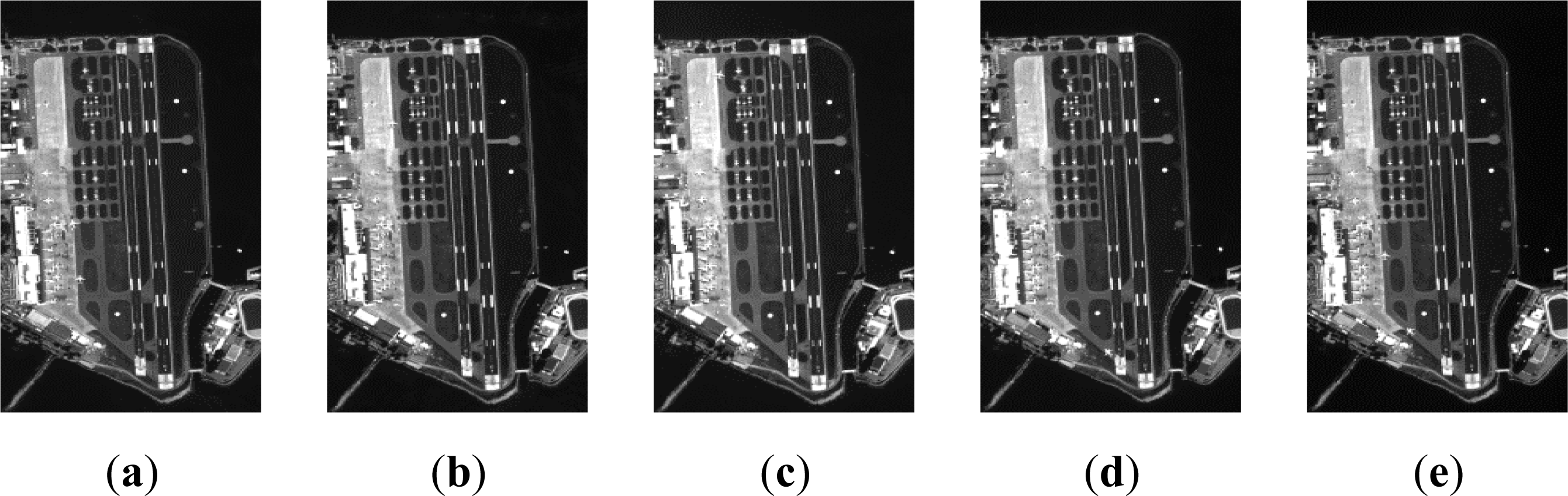
In this paper, for the experiment data, we use the WorldView-2 data which were provided by DigitalGlobe for the purpose of the 2011 IEEE GRSS Data Fusion Contest. This dataset was acquired over the Santos Dumont Airport of Rio de Janeiro city, Brazil, in 19 January 2010, within a three-minute time frame. The WorldView-2 satellite provides five angular images, each of which contains an eight-band multispectral image with a spatial resolution of 1.8 m and one panchromatic image with a 0.5 m spatial resolution [26]. The eight bands of the multispectral image refer to Coastal, Blue, Green, Yellow, Red, Red Edge, Near-IR1, and Near-IR2. The sensor acquires different angle images at 44.7°, 56.0°, and 81.4° in the forward direction, and 59.8° and 44.6° in the backward direction. The five angles of the panchromatic image and Band 1 of the multispectral image are shown in Figures 3 and 4, respectively. The flat image regions are selected in the experiments, as image registration of the parallax areas is complicated.

For the SRR experimental setting, the experimental section consists of two parts: simulation images and real images. The simulation images are obtained by downsampling the already existing HR image. In the quality assessment of the reconstruction results, the original HR image is usually chosen as the target reference image, which provides more objective support and reliability for the quantitative evaluations. The real images are cut from the large experimental images, with respect to the same imaging site. The corresponding experimental results are evaluated with user-designed quantitative measures. The motivation behind this is that with the two types of image data source we can fully validate the effectiveness of the proposed method. The two different types of quantitative measures are introduced in the next subsection.

For the SRR simulation image data experiments, the resolution enhancement factor is set to 2 for the horizontal and vertical directions, respectively. Two experimental regions of the 81.4° angle image are cut from the panchromatic image shown in Figure 3 and are shown in Figure 5, with each image of a size of 200 × 200, and the image values ranging from 0 to 255. The steps of obtaining the simulated LR images from the HR images are as follows: (1) Crop the corresponding image areas to the 81.4° angle images, as shown in Figure 5, from the other four different angle panchromatic images; (2) The multi-angle image sequence is convolved with a Gaussian smooth filter point spread function (PSF) of size 5 × 5 with the variance equal to 1; (3) Downsample the images in both the horizontal and vertical directions by a factor of 2. In the simulation process, we utilize all five multi-angle HR images to simulate the corresponding multi-angle LR images, instead of the traditionally used single HR image. By doing so, the geometric disparity between the five original multi-angle HR images is maintained, and thus more precisely simulates real multi-angle imaging conditions. Here, we choose the 81.4° angle image as the reference image. Therefore, in the quantitative evaluations, the 81.4° angle HR image is chosen as the target image.

The real experimental region is cut from Band 1 of the multispectral image shown in Figure 4, with a size of 190 × 190 pixels. The resolution enhancement factor is set to 2 for the horizontal and vertical directions, respectively. In the real image data experiment, the estimation of PSF is an important process in multiple-image SRR. Generally speaking, there are two ways to derive PSF in the context of SRR. One way is to assume the PSF is unknown and then conduct blind SRR [31], and the other approach is to assume the PSF to be known prior to the SRR process [15,20]. In fact, the latter approach is more commonly used because of the high ill-posedness of the blind SRR model. With this in mind, we use a Gaussian smooth filter of size 5 × 5 with variance equal to 1, which is commonly used in image SRR, for all the different angle images in the real multi-angle image SRR.

In the data preprocessing, we use histogram matching to conduct relative radiometric correction between the different angle images. The frequency domain motion estimation method [21] is utilized to perform the image registration, and the related registration accuracy analysis for the simulation images is given. The regularization parameter selection method in this paper is that several different regularization parameters are employed, and the parameter values corresponding to the best result are chosen. The bilinear interpolation result and the SRR result via the optimization of the general SRR model, which is shown in Equation (5) and similar to the optimization model [18], are used as benchmark methods.

3.2. Quantitative Evaluation Factors

In order to evaluate the quality of the reconstruction image, we use the following five quantitative evaluation factors in the simulation image data experiments and the real image data experiments: ISNR (improvement in signal-to-noise ratio), PSNR (peak signal-to-noise ratio), and SSIM (structural similarity index), which require the original HR reference image, are the image quality indicators for the simulation image data reconstruction images; and CPBD (cumulative probability of blur detection) and Metric-Q, which do not need the original HR reference image, are used for the real image data experiment quality evaluation.

(1) Improvement in Signal-to-Noise Ratio (ISNR)

ISNR is widely used in image restoration tasks [19,27]. Let x be the original HR image, x̂ represents the SR results, and x₀ denotes the bilinear interpolated image, then the ISNR value can be expressed as:

$$\mathit{ISNR}=10\hspace{0.17em}{\text{log}}_{10}\frac{\sum _{i=1}^{r^2\mathit{mn}}{\left({\mathbf{x}}_i-{\mathbf{x}}_0\right)}^2}{\sum _{i=1}^{r^2\mathit{mn}}{\left({\mathbf{x}}_i-{\widehat{\mathbf{x}}}_i\right)}^2}$$

(12)

ISNR is used to evaluate the sharpness of the image. The higher the ISNR value is, the better the quality of the reconstruction image.

(2) Peak Signal-to-Noise Ratio (PSNR)

PSNR is very commonly used in the quantitative evaluation of SRR results and is based on the mean square error between the HR image and the SR image, with relation to the logarithmic of (2^t−1)² (the maximum square of the signal), where t is the number of bits for each pixel value. We generally use eight bits for representing each pixel, so the formula can be expressed as follows:

$$\mathit{PSNR}=10\times {\text{log}}_{10}\frac{{255}^2\times r^2\mathit{mn}}{\sum _{i=1}^{r^2\mathit{mn}}{\left({\widehat{\mathbf{x}}}_i-{\mathbf{x}}_i\right)}^2}$$

(13)

PSNR can be used to characterize the image distortion. A better SRR image will get a higher PSNR value.

(3) Structural SIMilarity Index (SSIM)

SSIM, as proposed by Wang et al. [28], has been widely used for the evaluation of the quality of reconstruction images. The SSIM value is similar to the evaluation of the visual interpretation and is defined as:

$$\mathit{SSIM}=\frac{(2{\mu }_{\mathbf{x}}{\mu }_{\widehat{\mathbf{x}}}+C_1)(2{\sigma }_{\mathbf{x}\widehat{x}}+C_2)}{({{\mu }_{\mathbf{x}}}^2+{{\mu }_{\widehat{\mathbf{x}}}}^2+C_1)({{\sigma }_{\mathbf{x}}}^2+{{\sigma }_{\widehat{\mathbf{x}}}}^2+C_2)}$$

(14)

where μ_x and μ_x̂ are the mean values of the HR image and the SRR image, respectively. σ_x and σ_x̂ represent the variance of the HR image and the SRR results, respectively. σ_xx̂ is the covariance between the HR image and the SRR image. C1 and C2 are constant values to prevent the equation from being meaningless (numerator and denominator not equal to zero). In the simulation experiments, we set the constants C1 and C2 to 0.01 and 0.03, respectively, and the dynamic range of the image is from 0–255. SSIM is an evaluation factor used to characterize the contrast, brightness, and structural similarity of an image. It ranges from 0–1, and the closer the value is to 1, the better the image quality is.

(4) Cumulative Probability of Blur Detection (CPBD)

The CPBD measure, as proposed by Narvekar et al. [29], is a classification-based metric and is mainly used to evaluate image sharpness. In the algorithm, each class is calculated, with five grades of “Bad”, “Poor”, “Fair”, “Good”, and “Excellent”. The main principle is expressed as follows:

$$P_{\mathit{BLUR}}=P(e_i)=1-\text{exp}(-{\left|\frac{w(e_i)}{w_{\mathit{JNB}}(e_i)}\right|}^{\beta })$$

(15)

$$\mathit{CPBD}=P(P_{\mathit{BLUR}}\le P_{\mathit{JNB}})=\sum _{P_{\mathit{BLUR}}=0}^{P_{\mathit{BLUR}}=P_{\mathit{JNB}}}P(P_{\mathit{BLUR}})$$

(16)

Where P_BLUR represents the probability of blur detection. w_JNB(e_i) is the just noticeable blur (JNB). w(e_i) denotes the measured width of the edge e_i. P(P_BLUR) represents the PDF value when P_BLUR is known. The CPBD value ranges between 0 and 1. The CPBD measure is mainly used to assess the clarity of an image, and its value is between 0 and 1. The higher the CPBD value is, the better the image quality is.

(5) Metric-Q

Metric-Q is mainly used in image evaluation without a reference image [30]. It is based on the singular value decomposition of the local image gradient matrix, with the evaluation of contrast and sharpness. It still works well on images with random noise and blur. It can be expressed as:

$$Q=s_1\frac{s_1-s_2}{s_1+s_2}$$

(17)

where s₁ and s₂ are the singular values of an image patch of the SRR result, which represents the energy in the directions of the dominant and vertical orientations of the local gradient field. We evaluate the image quality by comparing the value of Metric-Q. A higher Metric-Q index value indicates an image with sharper edges, and represents more contrast and sharpness in the image.

3.3. Simulation Image Data Experiments

3.3.1. Registration Accuracy

Image registration is a key step in the SRR process, and it directly affects the quality of the final reconstruction images. The 81.4° angle image is selected as the reference image, and the other four different angle images are registered with respect to the reference image. In order to evaluate the registration accuracy, the global spatial domain image registration work by Shen et al. in [15] is adopted as the benchmark. The reason behind this is twofold. First, the frequency domain image registration method and the spatial domain method in [15] both account for the global motion between images, and thus provide the comparability between the two methods. Second, the spatial domain method [15] and its variants have been widely utilized and have been proven to be effective in many natural and remote sensing image super-resolution reconstruction tasks [1,2,15,32]. We choose two image regions of size 100 × 100 pixels, which are downsampled from the two images of size 200 × 200 pixels, as shown in Figure 5, by a factor of 2, to independently test the frequency domain motion estimation method. The comparative results of the two image registration methods by standard deviation (STD) of the local displacements [18] are shown in

Table 1. Registration evaluation for the experimental images in terms of standard deviation in the simulation image data experiment.

		59.8°	44.6°	44.7°	56.0°	Average
Image1	S	4.1959	5.1746	6.7593	4.2888	5.1047
	F	3.7878	4.5955	6.3109	4.3925	4.7717
Image2	S	5.9631	7.8938	7.1052	4.4458	6.3520
	F	4.8602	7.0562	5.3140	3.7444	5.2437

.

In Table 1, the best registration evaluation results for the two image sequences are marked in bold. F represents the frequency domain image registration method [21], and S is the global spatial domain registration [15]. From the table, it is observed that the registration results of the frequency registration method are better than those of the global spatial domain registration method, which suggests that the frequency registration method is more appropriate for the SRR here. As the main focus of this paper is to validate the effectiveness of the proposed adaptive weighted super-resolution reconstruction method for a multi-angle image sequence, small and flat image regions are chosen in the reconstruction part. In the case of large-size multi-angle remote sensing images, the proposed weighted super-resolution reconstruction method can be utilized jointly with the image registration approach proposed by Ma et al. [18], for practical operational purposes.

3.3.2. The Evaluation of the Reconstruction Results

We now evaluate the multi-angle super-resolution reconstruction results of the two image sequences, which are given in Figures 6 and 7, respectively. The (a) and (b) images in Figures 6 and 7 show the original HR image and the bilinear interpolation results, respectively, and (c), (d), and (e) in Figures 6 and 7 show the results of the general SRR method (GEN), angular difference weighted SRR method (ANGW), and residual error weighted SRR method (RESW), respectively. From Figures 6 and 7, it is observed that the SRR results, both with weighting and without weighting, obtain more detailed information and better visual quality than the bilinear interpolation result. By considering the resolution differences between the different angle images, our proposed adaptive weighted SRR algorithm’s results are more similar to the original HR image than the non-weighted SRR algorithm, from the visual evaluation.

Three quantitative measures, ISNR, PSNR, and SSIM, are used to evaluate the quality of the reconstruction images, and the quantitative evaluation results are shown in

Table 2. ISNR comparisons of the reconstruction results in the simulation image data experiment.

	Bilinear	GEN	ANGW	RESW
Image1	0.0000	6.9709	7.3191	7.5331
Image2	0.0000	7.8626	8.2089	8.3915

Table 3. PSNR comparisons of the reconstruction results in the simulation image data experiment.

	Bilinear	GEN	ANGW	RESW
Image1	28.3764	35.4517	35.7889	35.9797
Image2	26.8861	34.6467	34.9311	35.0416

and

Table 4. SSIM comparisons of the reconstruction results in the simulation image data experiment.

	Bilinear	GEN	ANGW	RESW
Image1	0.9357	0.9682	0.9702	0.9711
Image2	0.9340	0.9672	0.9692	0.9704

, respectively. The best evaluation result for each image is marked in bold, and the second-best result is underlined.

Table 2 shows the ISNR results of the four resolution enhancement methods with the four images. Better reconstruction results are reflected by higher ISNR values. It is observed that the RESW SRR method achieves the best result on Image1 and Image2, and obtains an improvement averaging 0.55 dB. In general, the proposed adaptive weighted SRR methods obtain better ISNR quantitative evaluation results than the general SRR method.

The PSNR and SSIM results of the four images are shown in Table 3 and Table 4, respectively. Better reconstruction results are reflected by higher PSNR and SSIM values. It is observed that the RESW SRR method obtains the best results on Image1 and Image2. It is concluded that, by considering the resolution differences between the different angle images, the proposed adaptive weighted method outperforms the traditional non-weighted SRR method in terms of both visual evaluation and quantitative measures.

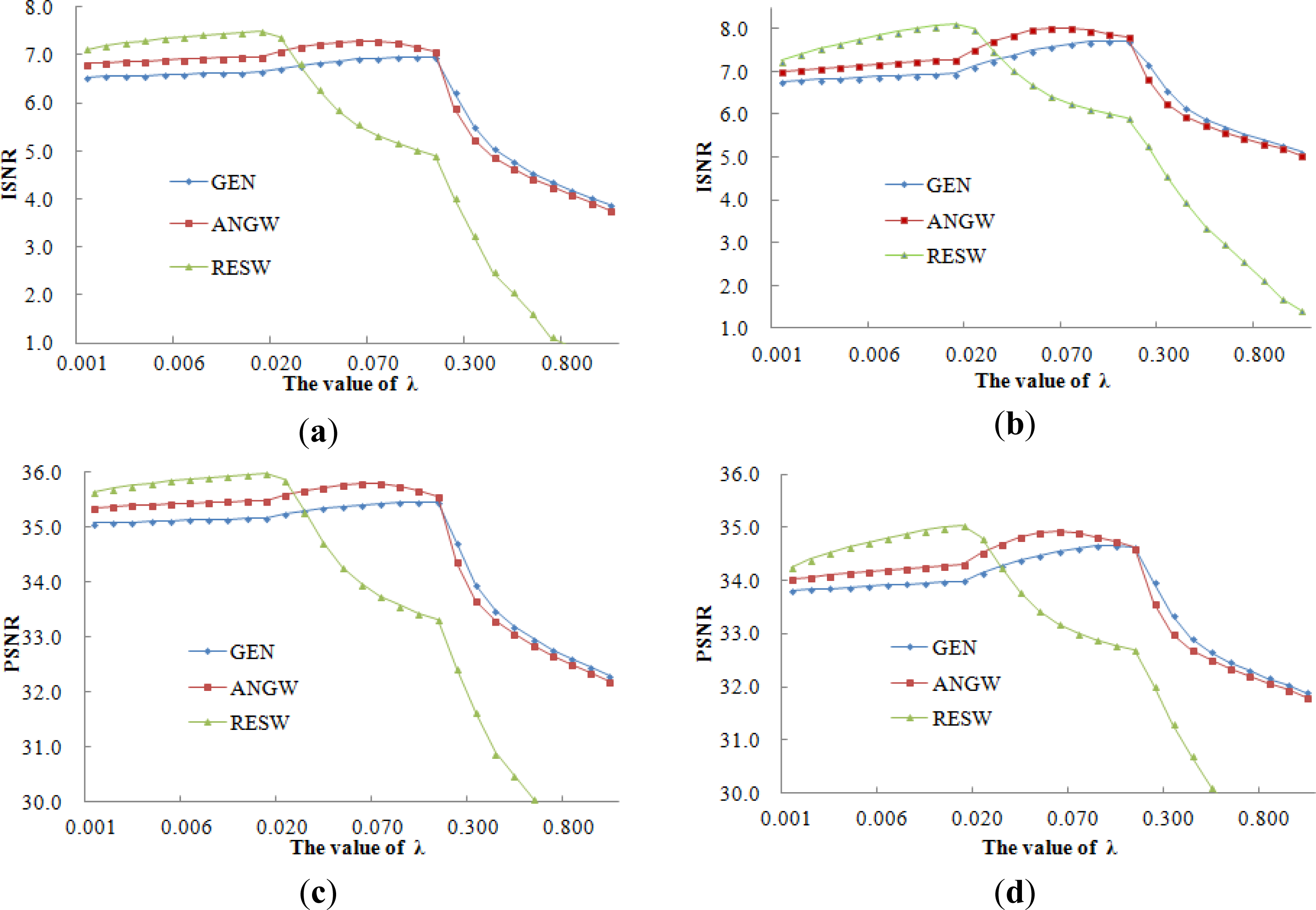
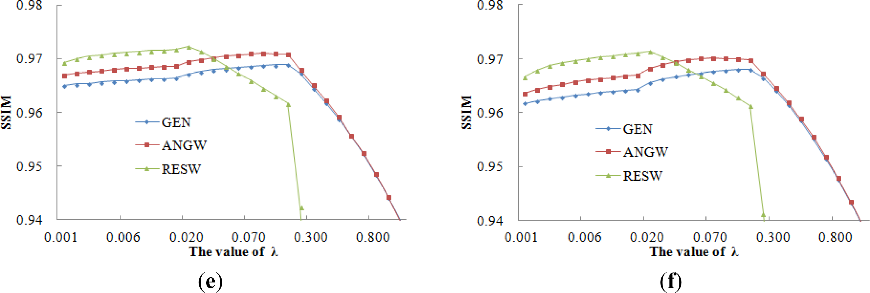
3.3.3. Parameter λ Sensitivity Analysis

To access the sensitivity to the regularization parameter in the SRR process, the relationships between the ISNR, PSNR, and SSIM values and λ are shown in Figure 8.

As shown in Figure 8, the horizontal axis represents the value of the regularization parameter λ, and the vertical axis shows the value of the quantitative evaluation factor. In all these six figures, it is shown that all three quantitative evaluation factors vary with the regularization parameter λ and share the same trend, which improves gradually until a certain point but drops after the top value and exhibits a parabolic-like curve. It is observed that the results of the three super-resolution reconstruction methods are quite robust to the variation in the value of the regularization parameter λ. In addition, the proposed two adaptive weighted SRR methods achieve better results than the general SRR method.

3.3.4. Contribution Analysis of Multi-Angle Images

To analyze the different contributions of the multi-angle images to the final SRR result, the weight values of each different angle image obtained by the two weighting schemes are shown in

Table 5. Weight of each angle image for the ANGW method in the simulation image data experiment.

Angle	81.4°	59.8°	44.6°	44.7°	56.0°
Weight	1.0000	0.8645	0.6412	0.6428	0.8160

and

Table 6. Weight of each angle image for the RESW method in the simulation image data experiment.

Angle	81.4°	59.8°	44.6°	44.7°	56.0°
Image1	1.4745	1.0040	0.7647	0.5485	1.2072
Image2	1.3571	1.1177	0.5667	0.6070	1.3515

, respectively. The weights for the multi-angle images derived by the ANGW method are the same for all the LR image sequences, and the weight combination obtained by the RESW method differs from the experimental data. From the tables, it is observed that the images which are closer to the nadir image achieve larger weights, which validates the effectiveness of the two weighted SRR methods from another perspective.

3.4. Real Image Data Experiment

The weight values of each different angle image obtained by the RESW method for the real image data experiment are illustrated in

Table 7. Weight of each angle image for the RESW method in the real image data experiment.

Angle	81.4°	59.8°	44.6°	44.7°	56.0°
Weight	2.0938	0.9510	0.4733	0.5210	0.9609

, and the weights of the ANGW method are set to the same as in Table 5. The observations from Table 7 are consistent with those of the simulation image data experiments. That is to say, the images which are closer to the nadir image achieve larger weights.

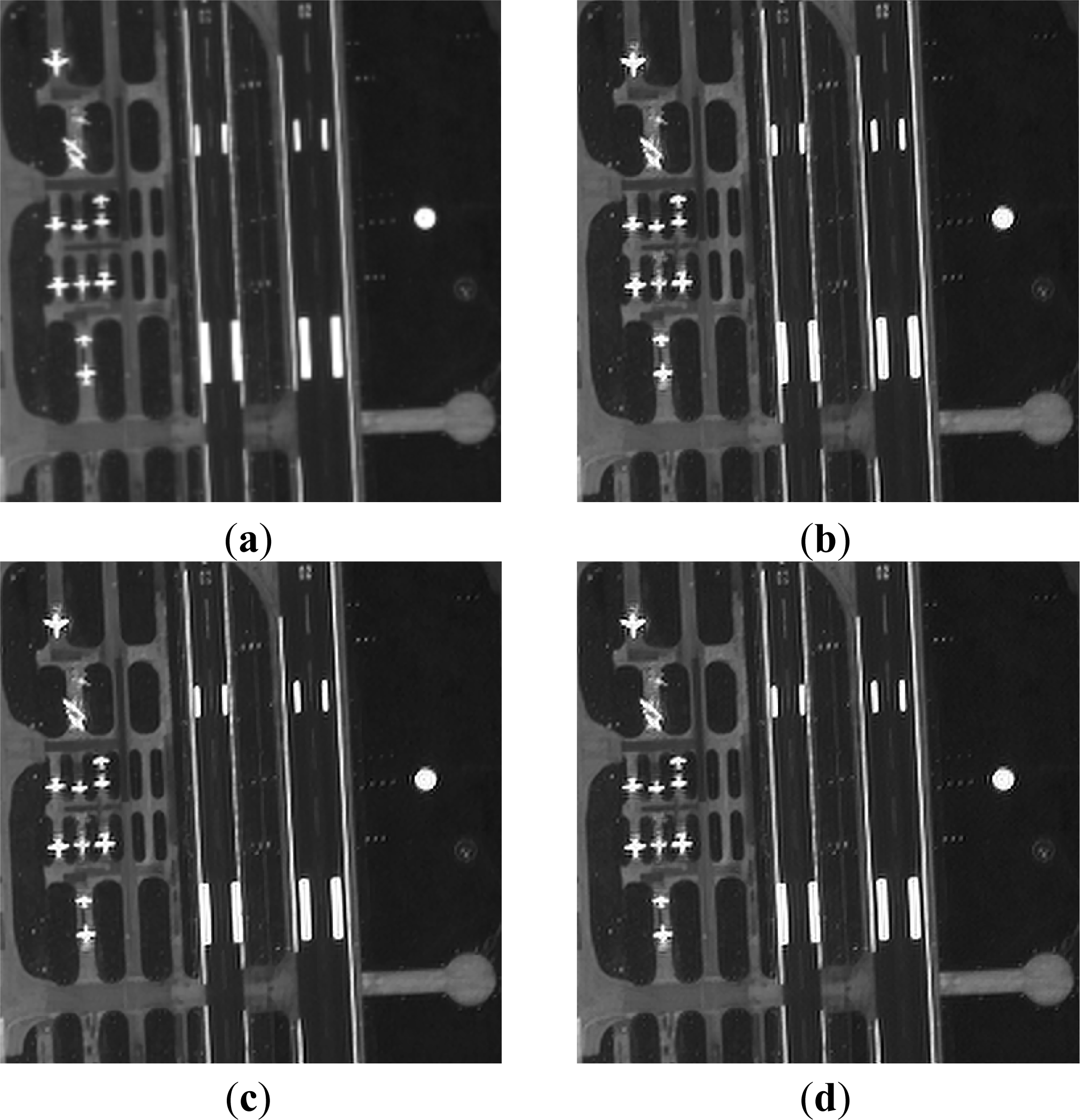
Figure 9a–d displays the SRR results of bilinear interpolation, the general SRR algorithm with no weighting, the ANGW SRR method, and the RESW SRR method, respectively. From Figure 9, it is observed that the three SRR results have a better visual quality than the bilinear interpolation result. To facilitate the visual comparison, four regions are cropped from the reconstruction result, as shown in Figure 10, and are illustrated in Figures 11 and 12, respectively.

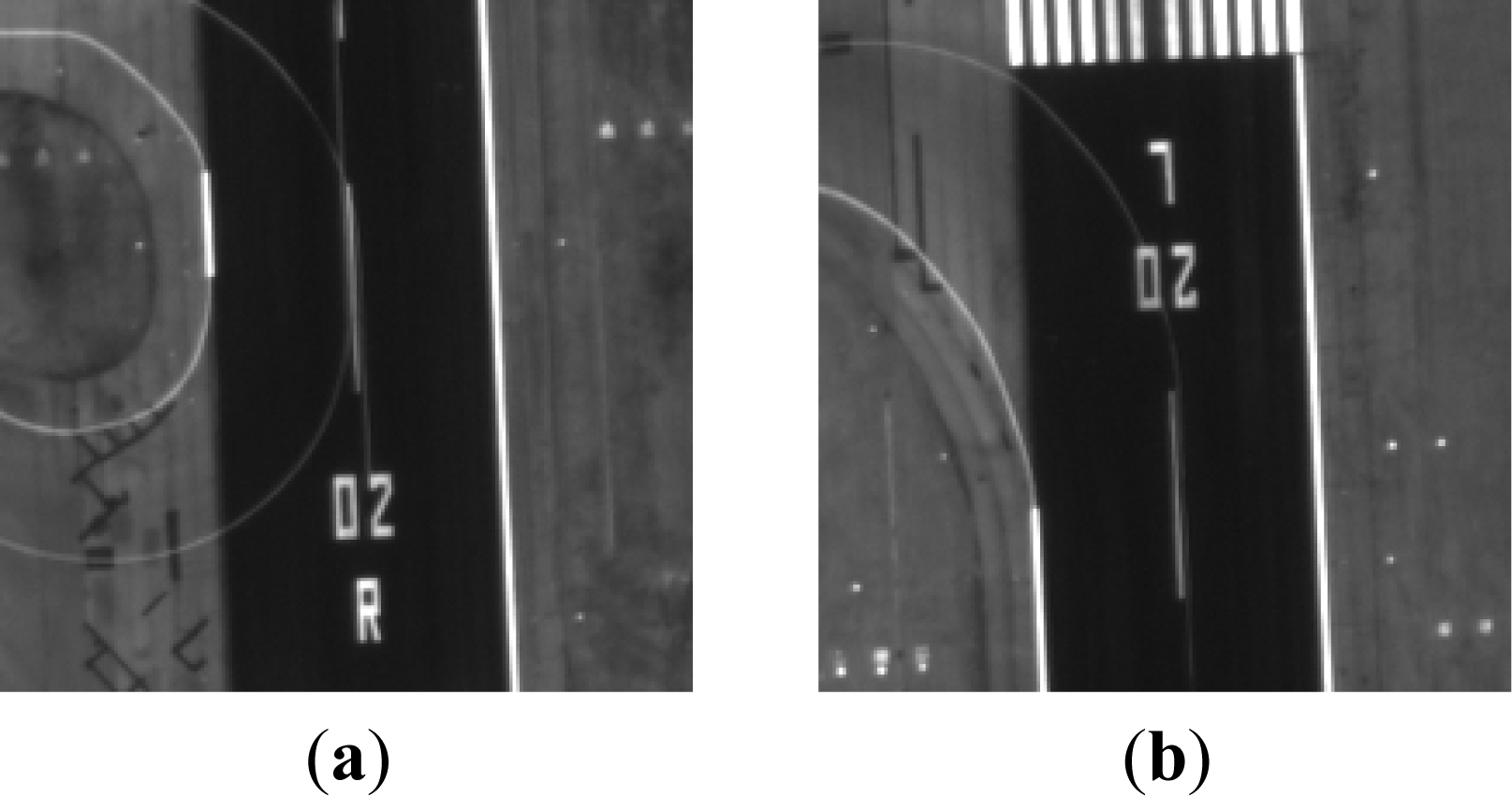
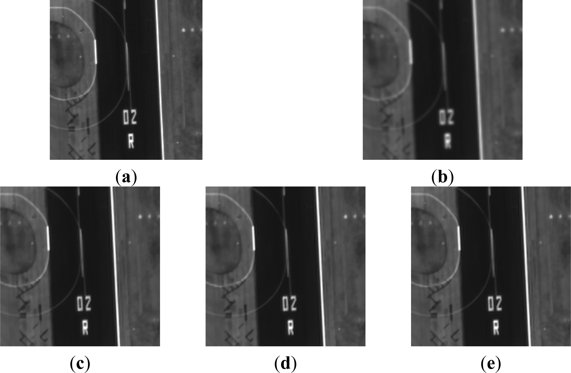
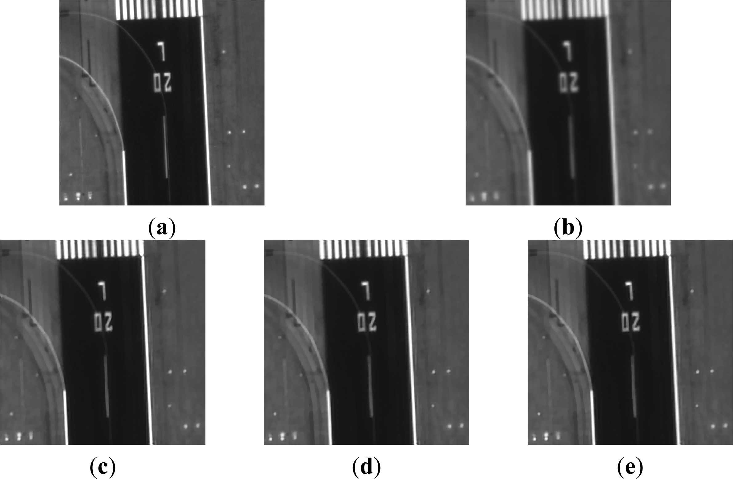
Images (a–e) in Figures 11 and 12 show the results of bilinear interpolation, the general SRR algorithm, the ANGW SRR method, and the RESW SRR method, respectively. Image (f) in Figures 11 and 12 shows the corresponding area taken from the panchromatic image as the ground truth reference. There are many detailed parts in the experimental results which can reflect the superiority of the two proposed adaptive weighted SRR methods over the general SRR algorithm. For example, images (d) and (e) in Figure 11 have richer details inside the circular flat area than Figure 11c, and the points distributed around the circle are brighter. The aircraft outlined in images (d) and (e) of Figure 12 have more sharpness and better continuity than the other results.

On the whole, it is observed that the results of the SRR methods, both with weighting and no weighting, have a much better visual quality than that of the bilinear interpolation. In addition, the results of the two adaptive SRR methods have slightly more sharpness, richer detailed information, and higher image contrast than that of the general SRR method, which confirms the feasibility and the effectiveness of the proposed adaptive weighted SRR methods.

In order to obtain a precise quantitative evaluation of the real image experiment results, the CPBD values and the Metric-Q quality evaluation results are shown in

Table 8. CPBD and Metric-Q of the reconstruction image shown in Figure 9.

	Bilinear	GEN	ANGW	RESW
CPBD	0.2775	0.6912	0.7079	0.7084
Metric-Q	35.1768	50.6106	50.7991	51.0615

. The best evaluation result for each image is marked in bold, and the second-best result is underlined. The quality of the reconstruction results is reflected by a higher CPBD value and Metric-Q value. Comparing the quantitative evaluation measurements in the first two columns of Table 8, it is observed that the reconstruction results of the general SRR method are much better than those of the bilinear interpolation method, which suggests that the complementary information from multi-angle images can be used to enhance the image spatial resolution. In the last three columns, it is observed that by considering the resolution differences of the multi-angle images, the two proposed adaptive weighted SRR methods further improve the reconstruction results.

4. Conclusions

Different imaging angles lead to spatial resolution differences between the images. To alleviate the negative effects of the resolution differences on the quality of the reconstruction image, we propose an adaptive weighted super-resolution reconstruction scheme for multi-angle remote sensing images. Specifically, two weighting strategies are introduced in this paper. The first method utilizes the angular difference between the imaging angles of the current LR image and the nadir image. The second weighting method determines the weight of one LR image as inversely proportional to its corresponding residual error. The proposed SRR model is composed of the ℓ₂ norm as the data fidelity item and the TV model as the regularization item, and is then solved with the steepest descent method. The results in both the simulation image data experiments and the real image data experiments confirm the feasibility and effectiveness of our proposed model, in terms of both the visual evaluation and quantitative measurements.

There is, however, still room for further improvement. For example, we only chose the flat regions in the experiments. The registration of the parallax areas is still a challenge, so more robust motion estimation methods are needed. In the imaging process, different angle images are degraded by different levels of blurring and noise, so the estimation of the PSF of each different angle image should also be taken into consideration.