Effects of Disturbance and Climate Change on Ecosystem Performance in the Yukon River Basin Boreal Forest

 ,
,
Abstract
: A warming climate influences boreal forest productivity, dynamics, and disturbance regimes. We used ecosystem models and 250 m satellite Normalized Difference Vegetation Index (NDVI) data averaged over the growing season (GSN) to model current, and estimate future, ecosystem performance. We modeled Expected Ecosystem Performance (EEP), or anticipated productivity, in undisturbed stands over the 2000–2008 period from a variety of abiotic data sources, using a rule-based piecewise regression tree. The EEP model was applied to a future climate ensemble A1B projection to quantify expected changes to mature boreal forest performance. Ecosystem Performance Anomalies (EPA), were identified as the residuals of the EEP and GSN relationship and represent performance departures from expected performance conditions. These performance data were used to monitor successional events following fire. Results suggested that maximum EPA occurs 30–40 years following fire, and deciduous stands generally have higher EPA than coniferous stands. Mean undisturbed EEP is projected to increase 5.6% by 2040 and 8.7% by 2070, suggesting an increased deciduous component in boreal forests. Our results contribute to the understanding of boreal forest successional dynamics and its response to climate change. This information enables informed decisions to prepare for, and adapt to, climate change in the Yukon River Basin forest.1. Introduction
Ecosystem productivity in the boreal forest is often constrained by short growing seasons, lack of winter sunlight, temperature, permafrost, low soil nutrient levels [1,2], and disturbance [3–5]. Furthermore, ecosystem productivity is increasingly limited by mid-summer moisture stress [6–9]. Northwestern North America (and northern latitudes in general) is predicted to continue warming throughout the 21st century, and climatic changes over the last century have already resulted in warmer springs accompanied by an earlier start of growing season [4,10], warmer summers, and much warmer winters [11]. Altered weather patterns are due in part to the shift in the Pacific Decadal Oscillations (PDO) in the 1970s [12]. These changes, combined with ongoing warming, will likely alter the structure [13,14], composition [15,16], distribution [7,17,18], disturbance regimes (increasing severity and frequency of insect outbreaks and fire) [15,19,20], ecosystem services or productivity [2,21–23], postfire succession [24], and ecosystem goods and services of the boreal forest.
Warming and drying weather conditions throughout the 20th century have been linked with reduced radial growth of white spruce in the Alaskan boreal forest [6]. Remote sensing studies have observed similar patterns of boreal “browning” since the 1980s [9,25]. The warming climate may change the limiting factor of tree growth from temperature to moisture [2,7,23], particularly in mid-summer [7,26]. These changes will likely result in increased burned area, fire frequency, and fire severity [27]. Severe fires often expose bare mineral soils in which deciduous propagules have great success [28] and dominate early to mid-successional communities [29] and result in increases in long-term deciduous forests. Boreal deciduous species have been reported to respond more positively to climate change [15,16,25] and drought [30] than boreal coniferous species, and are likely to increase in a warmer climate [16,20,28,31–33]. Since mature deciduous stands often have greater ecosystem productivity [5,16,29,33,34], greater carbon uptake [30,35,36], and a longer fire return interval than coniferous stands, an increase in their cover/extent is likely to increase overall ecosystem productivity. While climate change may be associated with decreasing coniferous productivity and abundance, its net effect on overall long-term boreal productivity is uncertain. The strength and direction of future productivity patterns in the boreal forest depends largely on changes to the quantity and timing of precipitation, continuing increases in greenhouse gases, the strength of the CO2 fertilization effect [22], species diversity and beneficial interactions [37], PDO patterns, and corresponding changes to the disturbance regime [20].
Interannual variation in weather influences the temporal signal of vegetation recovery following a disturbance event [17] and obscures ecosystem “performance”, or productivity, trends related to succession and climate change [8]. How well vegetation responds to growing conditions such as weather and site conditions (soils, elevation/aspect, permafrost, etc.) is described here as “ecosystem performance”, which is assessed with growing season integrals of remotely sensed vegetation indices [38–41] that are associated with photosynthetic potential or vegetation greenness. Healthy, robust vegetation will respond to moisture stress, insect infestations, and other plant stressors in a robust manner (normal performance) while a degraded or previously stressed vegetation stand may have a larger reduction in productivity given the same stressors (underperformance). Disturbances such as stand replacing fires will be readily represented as severe performance departures from that expected for a mature forest given site conditions. Environmental thresholds use a similar concept of the “degree of vegetation stress” or “accumulation of stress factors” to identify environmental stress loads that are critical for ecosystem failure or ecotype conversion [42].
Detecting significant temporal patterns in ecosystem performance is especially challenging because of the substantial [43,44] and increasing role of fire disturbance [3] and insect damage [4,20]. Interannual weather variations [19], often related to the PDO [23] also confound the temporal patterns in performance. To reduce the complex response of ecosystem performance to these factors [3], we used ecosystem models that account for variations of weather in moderate resolution satellite imagery and built upon the methodology of previously successful efforts [5,39] that tracked forest fire succession and grazing effects in the central United States [40]. Similar approaches that detrend spectral responses for weather and site conditions to assess range condition and management effects have been applied in Africa [45–47] and Australia [48]. The separation of climate and human influences through this approach combined with entropy analysis was also proposed by Zurlini et al. [49] as a method to identify causes of change. Our objectives were to (1) evaluate boreal forest performance departures from expected conditions in the Yukon River Basin over the 2000–2008 period; (2) separate the influence of weather on performance to reveal disturbance; (3) assess successional dynamics of ecosystem performance following fire using a chronosequence; and (4) model future equilibrium (non-disturbed) ecosystem performance in 2040 and 2070. .
2. Methods
2.1. Study Area
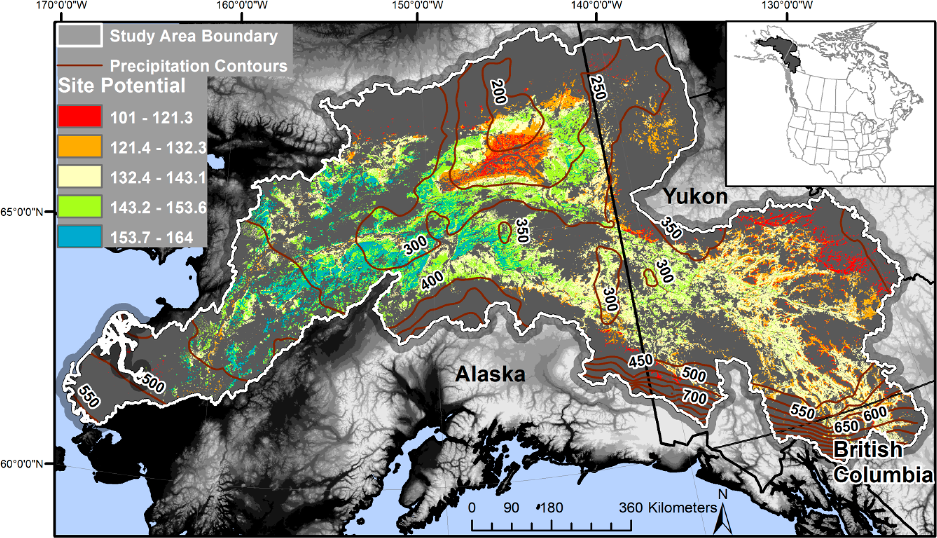
The Yukon River Basin encompasses 856,930 km2 of Alaska, USA, and Yukon and British Columbia, Canada (Figure 1). We evaluated the portion of the basin that was either boreal forest (i.e., 2001 National Land Cover Database (NLCD) coniferous or mixed forest; overall accuracy for these forest classes of 76.4% [50]) or potential boreal forest (e.g., areas recovering from disturbance) (Figure 1). The evaluated area encompassed 32% (280,149 km2) of the basin. Potential boreal forest was determined with a combination of the 2001 NLCD, Global Land Cover (GLC) 2000 [51], Alaska 1980s land cover, and the International Geosphere-Biosphere Programme MODIS land cover to identify areas with long-term boreal forests and exclude fire effects. Boreal forest in the Canadian portion of the watershed was determined solely from the GLC 2000 data.
Boreal forest in the Yukon River Basin is dominated by coniferous species including white spruce (Picea glauca Moench) and black spruce (Picea mariana Mill) [29,34]. Deciduous species such as aspen (Populus tremuloides Michx.), Alaskan birch (Betula neoalaskana Sarg.), paper birch (Betula papyrifera Marshall) and balsam poplar (Populus balsamifera L.) are frequently associated with earlier successional communities following fires [4,52,53] and south-facing aspects [29], often mixing with coniferous species [44] in mid-late successional stages.
The average winter temperature within Yukon River Basin boreal forest is −17.6 °C, while the summer average ranges from 8 °C to 16 °C and the yearly average ranges from −7 °C to 6 °C [29]. Average annual precipitation varies geographically from 150 to 565 mm, with the highest amounts occurring along the Alaska Range [54]. Precipitation generally decreases from west to east (Figure 1). Mountain ranges restrict the maritime influences carrying moisture, resulting in regions where potential evapotranspiration is greater than precipitation [1]. Generally, permafrost is continuous north of the Yukon River, and discontinuous to the south [11,55].
2.2. Ecosystem Performance Modeling
Our ecosystem performance assessment consists of four steps (after [5]): (1) determine the actual ecosystem performance; (2) compute long-term site potential; (3) model Ecosystem Expected Performance (EEP) given long-term site potential conditions, yearly weather, and assuming no disturbance occurs; and (4) calculate Ecosystem Performance Anomaly (EPA) as the difference between actual and expected ecosystem performance.
2.2.1. Actual Performance
Ecosystem performance (EP), or actual performance, is represented by the growing season integral of the Normalized Difference Vegetation Index (GSN). The Normalized Difference Vegetation Index (NDVI) has been related to chlorophyll [56], nitrogen stress [56], fractional vegetation cover [56], Leaf Area Index (LAI) [56], gross primary production [56], and foliar water potential [56]. NDVI also tracks vegetation dynamics related to phenology [57,58]. Growing season summaries of remotely sensed vegetation indices capture vegetation dynamics through the growing season [57,59,60], including shoulder season dynamics that are sensitive to climate instability [56,57]. Growing season integrals of vegetation indices have been related to or used as relative proxies for total standing biomass [61–63], photosynthetic activity [64,65], biological activity [66], productivity [57], forest foliar productivity [67], biomass [62,68], primary production [7,25,27,45,69], fire succession [70], and LAI in deciduous and coniferous boreal forests [71].
The 250 m Moderate Resolution Imaging Spectroradiometer (MODIS) data, with a temporal (weekly) resolution, capture local variability in productivity and are appropriate for evaluating the impacts of climate change and forest stress. The 250 m expedited MODIS (eMODIS) [72] 7-day NDVI composites were rescaled from the NDVI’s −1 to 1 range to 0 to 100, and all negative values (clouds and water) were set to 0. Soil and litter effects were minimized by subtracting 0.09 from NDVI values [73] and to improve GSN sensitivity to vegetation [69]. These NDVI composites incorporate data quality information related to clouds, view angles, and snow [74] and were temporally smoothed [75] to remove any remaining cloud effects for each growing season, defined as 1 April to 30 September. Temporal smoothing of NDVI spans temporary drops in NDVI related to residual clouds which can remain after the 7-day maximum NDVI compositing process. A series of linear regressions from a moving temporal window are used to estimate “fill in” appropriate NDVI values for periods of temporarily low NDVI values [75]. To capture interannual productivity variations in the shoulder seasons and capture growing season length changes, a constant time window for NDVI averaging was employed (1 April to 30 September). The high temporal resolution of the eMODIS data utilized in this study was critical to capturing these patterns [70]. Growing season average NDVI (GSN) with a constant growing season period is algebraically consistent with the sum of NDVI over the growing season and emphasizes the importance of the length of the productive period and the effects of varied shoulder seasons [10]. A varied growing season length used in the average would tend to standardize for growing season length, resulting in potentially similar GSN values for a short growing season and a long growing season with similar weekly NDVI magnitudes during the growing season. By using eMODIS NDVI, the MODIS swath data were directly projected to Alaska Albers Equal Area [74], avoiding geographic distortions associated with the extreme latitudes and longitude in the global sinusoidal projection for this study area [72,76,77].
2.2.2. Models
The basic modeling approach is a regression tree EP model based on the basic hypothesis that Actual Performance is a function of site potential and weather. Site potential is the long-term GSN estimated through a regression tree driven by time invariant spatial data sets related to site condition (elevation, soils, aspect, etc.). Once site potential is mapped, it does not vary between years and is used as a driver in the EP model to represent the combined effects of site differences on boreal forest long-term productivity, Site potential should account for most of the geographic variation and allow the weather data to address interannual variations.
Data-driven, machine learning regression tree models were used to develop models for predicting both site potential and EP. Rule-based piecewise regression techniques were employed to model the nonlinear response of long-term average ecosystem performance and annual ecosystem performance. To maximize prediction accuracy and insure model robustness, we used multiple models each with high numbers of terminal nodes and multiple regression equations, which allowed for only the most useful variables to be used in different environmental settings. This modeling approach enables the automatic handling of interactions, since different linear regression models are used in different parts of the predictor variable space [78]. This approach often results in better prediction accuracy [79] than a single multivariate linear regression. For a detailed description of the piecewise rule-based regression tree, see [5].
Two regression tree mapping models were constructed: (1) site potential, which represents the long-term (2000–2005) average expected performance for each site (primarily geographic variability); and (2) EP model, which included site potential as an input and employed yearly weather to address interannual variability. Site potential and EP were spatial dependent variables that can be reliably replicated through time and space [5,80]. Stratified random sampling for the site potential model (n = 2529) was done to insure near-equal representation of the model development database sample locations in low, moderate, and high productivity areas to help minimize prediction bias. The EP model included years as an additional stratification criteria (n = 15,049). To focus the EP model predictions on mature boreal forests all sample points were further constrained to exclude areas that had burned in the previous 50 years. Fire perimeters were obtained from the Bureau of Land Management, Alaska Fire Service [81], and the Canada Forest Service. The relatively large model development data sets helped to insure that the models were robust to a wide range of conditions. Inputs to the site potential model included temporally static variables that characterized site conditions: soil drainage, land forms, elevation, aspect, slope, compound terrain index, surficial geology merged from two sources [82,83], ecoregions [84], median potential evapotranspiration [85], environmental domains [85], median solar radiation [85], permafrost characteristics [86], and historical monthly climate grids for North America [87].
2.2.3. Ecosystem Performance Anomalies (EPA)
GSN (actual performance) was regressed on EEP (expected mature forest performance) to assess model prediction accuracy and to derive the 90% confidence limits for the regression. Data points that fell below the regression line were underperforming relative to an undisturbed boreal forest but only significant (p < 0.10) when they were below the lower 90% confidence interval. The inverse would be for overperforming observations being above the regression line and above the upper 90% confidence interval. Between the upper and lower confidence interval (±69 in rescaled NDVI units) was considered mostly the range of normal performance variability and pixels that fell outside the 90% confidence intervals were Ecosystem Performance Anomalies (EPA) [41]. Picking a level of significance can be user specific so EPA map color ramps show graduations but all significant anomalies were red tones or green tones and labeled as two levels of significant overperformance or underperformance. EPA are essentially the residuals of the GSN regressed on the EEP model predictions, which were significant outliers at p < 0.10. Maps of EPA were produced for each year. Setting a confidence limit threshold standardizes the sensitivity of the EPA to the EEP model error and provides quantification of both anomaly magnitude and a statistical significance of anomalies. Since the EEP model largely accounts for both site conditions (though the site potential variable) and weather, EPA values are standardized, detrended, or normalized for weather and site conditions resulting in an interannual and spatially consistency that facilitates interannual comparisons and analysis.
2.2.4. Future Ecosystem Performance
Future (2040 and 2070) EEP was determined using the same model we employed for the 2000–2008 annual EEP products. However, for mapping the future EEP, we replaced contemporary weather conditions with the future climate projections of a 14-model average composite generated following the assumptions of emissions scenario A1B [88] for 2040 and 2070. The resulting EEP values in 2040 and 2070 were compared to the 2000–2008 average, to generate a percent difference map. Future EEP values represent the potential mature forest performance of a site in the absence of disturbance (fires and insects). The future EEP values carry the assumption that the current performance-weather relationship (which captured interannual moisture and temperature variations and gradients in a large and diverse study area across multiple years) informs response predictions for future environmental conditions. The frequency and magnitude of extrapolation of the EEP model (model application beyond the data range that it was developed from) when applied to future climate projections was assessed using an extrapolation differencing approach [89]. A difference map of an EEP that allowed a 50% extrapolation beyond the model development data range and one that constrained extrapolation to 10% extrapolation quantified the spatial frequency and the magnitude of extrapolation in the future EEP predictions. Our modeling constrained boreal forests to their original (2000–2008) extent and did not consider possible range expansions or contractions.
2.3. Forest Succession
We evaluated the magnitude of disturbance from fire, and the subsequent recovery of EPA, using Alaska Fire Service fire perimeters from 1950 to 2002 available for the Alaskan portion of the study area. We employed a space-for-time design, or chronosequence, to study the pattern of succession following fire, specifically its influence on EPA and land cover proportions. This design assumes that observing the conditions at stands of varying ages (through space) would provide the same result if site(s) were observed throughout the entire post-disturbance recovery (through time). This assumption can be problematic at times [90]. However, this assumption was determined to be valid in boreal forest [53,91] in which chronosequences have often been used [25,92].
NLCD 2001 classes were sorted into four land cover groups; deciduous forest, coniferous forest, mid-succession (shrub and mixed forest), and early-succession (barren, grassland, sedge, and moss). Random points (n = 5000) were placed within fires over 200 ha in size occurring between 1950 and 2002. We believed this number of samples was sufficient to effectively quantify the population. These points were used to calculate the average EPA of each land cover group and the proportion of fire scar area in each for years before and after fire. Areas that burned more than once during the 1950–2002 period were excluded in an effort to clarify successional patterns following fires and to reduce fire-related changes to NLCD land cover. Burn severity (i.e., dNBR) was not considered in random point placement; consequently, our random points represent the entire range of burn severity within burned areas. We did not consider dNBR because (1) its accuracy has often been challenged in Alaskan boreal forest [93]; (2) it is unavailable for older fires (pre-1984); and (3) we wanted to represent the entire range of fire severity. Data from 2003 to 2008 were not used because the accuracy of NLCD 2001 likely diminished as later fires and succession continued to alter land cover. Only fires that occurred from 2000 to 2002 had observations of pre-fire and year of burn EPA. These data were used to generate scatterplots of average EPA and proportion of fire scar area and group by year since fire. The low sample size in some periods (e.g., 40–45 years since fire) caused greater variability in EPA.
2.4. Validation
Data-driven piecewise regression models (Cubist) were assessed with 10-fold cross validation and used multiple test data sets to assess model (constrained to the same inputs) accuracy and robustness [5,44]. Multiple random test data sets insured that validation results were representative of the larger population being mapped. We used total aboveground biomass data representing an average of 2008–2010 conditions for the Yukon Flats (the dry north-central portion with low site potential (Figure 1)) portion of the basin [44] to validate the ability of the GSN to serve as a proxy of ecosystem performance. Estimates of AGB were previously derived for the area using Landsat TM data and in situ data, as described in [44], and were aggregated here to MODIS pixel sized areas by averaging the biomass 30 m pixels within each 250 m MODIS pixel. Linear regression was used to determine the relationship between GSN and aboveground biomass at random points (n = 545) located in areas of boreal forest in the Yukon Flats.
3. Results and Discussion
3.1. Site Potential and Expected Ecosystem Performance
Site potential was estimated using temporally static inputs that accounted for 49% of the variation in site potential (Figure 1, R2 = 0.49, n = 2529, p < 0.0001). Coarse resolution inputs (permafrost, long-term climate, surface geology) prevented the model from explaining higher amounts of 250 m GSN variability since GSN captures a significant amount of local variability. Fire perimeters also had larger errors for older fires and some fires were mapped before they were completely extinguished so outlier pixels could include some burned pixels.
Site potential tends to coincide with the east to west moisture gradient in the Yukon River Basin (R2 = 0.26, p < 0.01) due to the isolation of eastern areas from maritime moisture [1] (Figure 1). Low precipitation impacts are especially apparent in the Yukon Flats region in the north-central part of the Yukon Basin and in east-central Yukon, Canada, which has some of the lowest site potentials in the basin attributable to their continentality and rain shadows that reduce precipitation. Elevation was negatively related to site potential (R2 = 0.21, p < 0.01). In contrast to longitude, site potential was not significantly related to latitude, due to the confounding effects of elevation and the proportionately small latitudinal range of the study area. Site potential tends to be highest on floodplains and mid-successional deciduous forest. Our results commonly demonstrated low site potential in wet coniferous forests, while deciduous stands of aspen and birch were considerably more productive than white and black spruce [29], and had the highest site potentials, similar to [5].
3.2. Expected Ecosystem Performance
The EEP model had an R2 of 0.53 (p < 0.0001) from 15,049 spatially and temporally stratified locations across the study area. Extrapolating weather in Alaska is problematic because of the low density of weather stations especially at high elevations, which also contribute to EEP model outliers. The EEP model was also impacted by burn perimeter boundary errors. A 10-fold cross validation of EEP demonstrated equivalent prediction accuracy for unseen data to training data and demonstrated the robustness of the EEP model to the wide range of environmental conditions in the study area through time.
The EEP time series was grouped into 22 natural classes with similar time series trends with an unsupervised cluster analysis [94]. A review of the temporal signatures of these 22 classes showed that some of the classes were characterized by a significant drop in EEP in 2004, a record fire year in interior Alaska (Table 1). The clusters with this significant drop of EEP in 2004 were combined into a drought group and those without the 2004 EEP drop were put in a non-drought group. These two groups were overlaid with the 2004 fire perimeters and the percentage of area burned in 2004 for each group was calculated. The drought group had 24% of its area burned and was concentrated on the north and central to eastern parts of the Yukon River Basin. The non-drought group had 5% of its area burned and was concentrated on the southern part of the area with northward extents in western and a small part of central Yukon River Basin. The higher probability of 2004 fires in areas with a significant drop in 2004 EEP supports the EEP models ability to track moisture stress in this boreal system and demonstrates drought and fire associations in the Yukon Basin.
3.3. Ecosystem Performance Anomalies
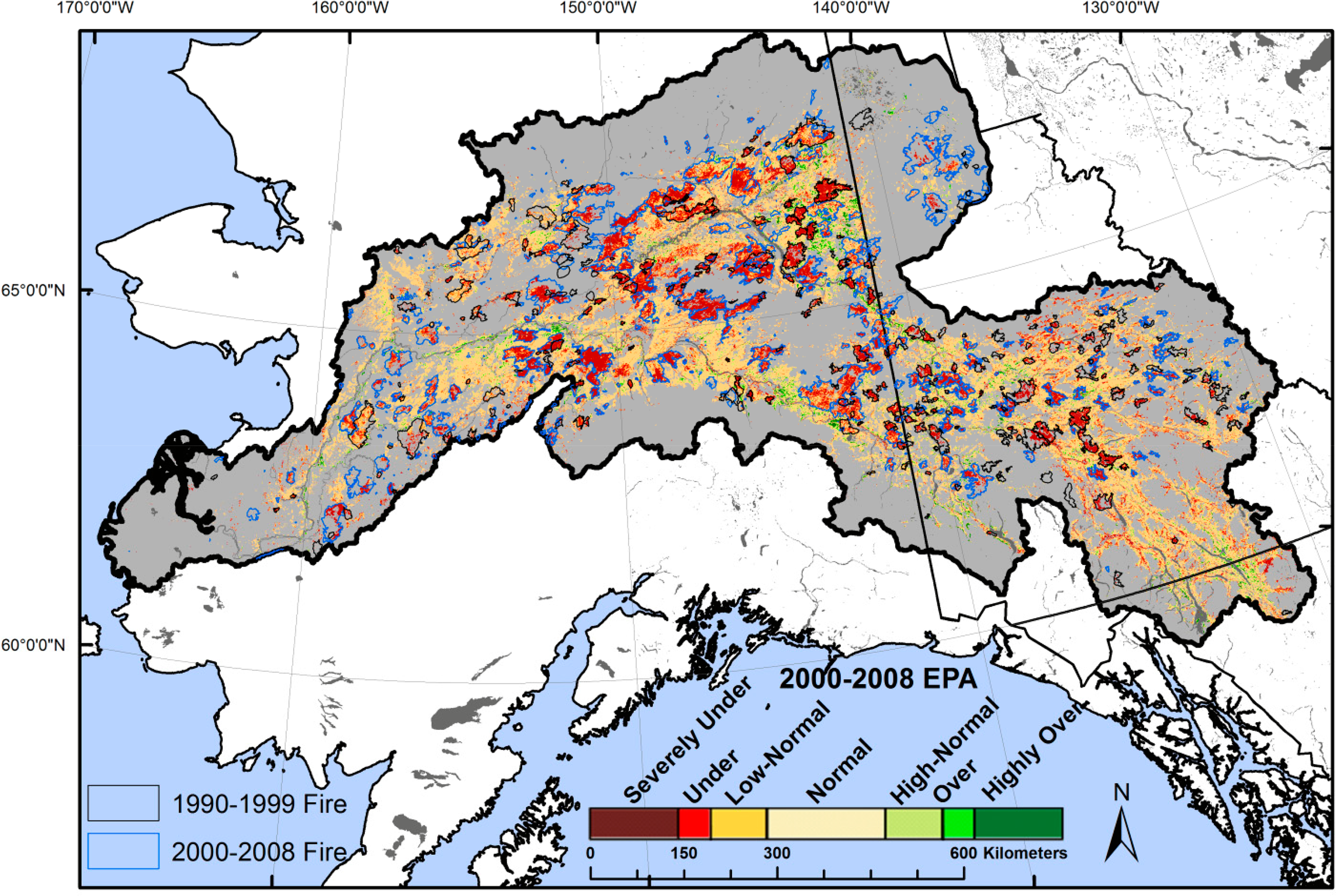
The 2000–2008 average EPA values were averaged and grouped into seven classes based on the relative confidence of their anomaly from expected values: severe under and over performance (95% confidence limits), under and over performance (90% confidence limits), low-normal and high-normal (80% confidence limits), and normal (<80% confidence limits) (Table 1). Because the EEP and site potential models are developed from unburned areas, a disturbance often generates a statistically significant negative EPA, as the EEP model does not ‘expect’ the disturbance because it is driven by only weather and site conditions and trained on unburned pixels. Since early successional stands were excluded from model development, the EEP model reflects an undisturbed/mature stand performance, allowing successional dynamics (normalized to yearly weather variations) to be represented as anomalies from mature forests.
Annual maps of the model residuals (EPA) indicated that 72.7% of the evaluated boreal forest performed normally (within the 90% confidence limits) when averaged over the study period (Figure 2), while individual years tended to have a lower percentage (∼60%) in the range of normal EPA values (Table 1). Years that had a low percentage of normal performance tended to be associated with years of high fire occurrence (e.g., 2004) and those immediately following a fire (e.g., 2005). The distribution of EPA values was strongly skewed toward underperformance (Table 1), with an overall average value of −28.7 due to disturbance [43] (Figures 2 and 3). For example, the 2000–2008 average EPA was underperforming in 23.4% of the study area, far more than the 3.9% occupied by overperforming classes (Table 1, Figure 2). The majority of EPA perturbations were caused by fires and insect outbreaks (insect damage perimeters were from the Alaska Department of Natural Resources) [5]. Correspondingly, the relationship between current plus previous year percent area burned and proportion of EPA in severe underperformance follows a positive linear relationship (R2 = 0.70, p < 0.05). The years 2007 and 2008 appeared to be outliers, with a higher than average proportion of overperforming EPA values. This overperformance may be due to the dominance of productive herbaceous vegetation and liberation of nutrients in areas impacted by 2004 and 2005 fires.
The 2000–2008 average EPA in coniferous forest was −1.5 (±3.5 SE). Our model development occurred in areas of coniferous and mixed forest that were not recently disturbed, hence the average coniferous EPA near zero indicated that our model performed as expected. EPA values could therefore also be thought of as the performance departure from the conditions expected of an undisturbed coniferous stand. Deciduous stands for example, had an average EPA of 33.8 (±2.7 SE), suggesting greater ecosystem performance than coniferous forest, a commonly reported finding [5,16,29,34]. This is partly driven by higher deciduous productivity [29], but also by higher near-infrared reflectance and higher NDVI from broadleaf vegetation than need leaf vegetation. This near-infrared reflectance difference is driven by the broadleaf mesophyll internal structure [56]. This pattern is supported by Figure 3, which demonstrates that areas of deciduous forest tended to be overperforming or highly overperforming. Areas within river meanders, oxbows, and areas of moist soils also tend to be overperforming because these sites are protected from fire, allowing them to mature longer than the study area average. To validate our EPA results, we compared GSN, our proxy of actual ecosystem performance, to Landsat-derived aboveground biomass measurements for the Yukon Flats area [44]. This comparison yielded a moderately strong linear relationship (R2 = 0.47, p < 0.01), indicating that GSN is a reasonable proxy of ecosystem performance.
3.4. Impacts of Fire
3.4.1. Impacts on Ecosystem Performance Anomalies
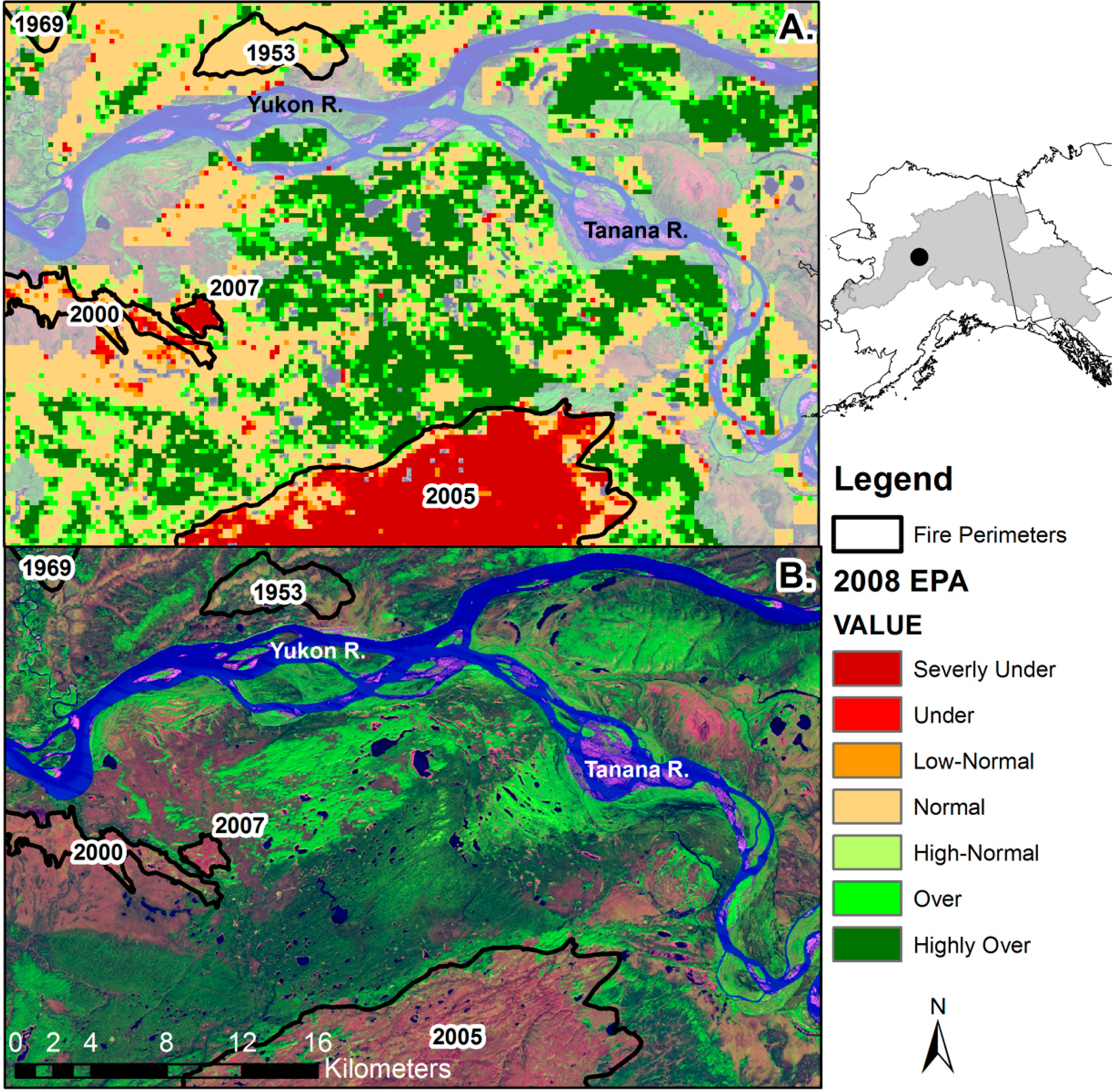
Species composition, stand age [14,52], carbon dynamics [43,53], permafrost condition, and performance [44] are often modulated by fire in the boreal forest. Fires are the dominant disturbance in the boreal forest [43]; 47% of the Yukon River Basin boreal forest burned at least once between 1950 and 2008 and 16% burned at least twice. Estimated fire return intervals in the Alaskan boreal ecoregions ranged from 74 to 326 years from 1950 to 2009 [27]. Fires create a landscape mosaic of large patches in various stages of succession following fire (Figures 2 and 3). Figure 3A depicts severely underperforming EPA within fire scars 1 and 3 years old, while the area within an 8-year-old stand had recovered slightly to include normal and under-performance (Figure 3A). Mid-successional stands, 39 and 55 years old, were indistinguishable from the surrounding landscape and contained areas of normal and overperforming EPA, similar to the pattern seen in Figure 4A.
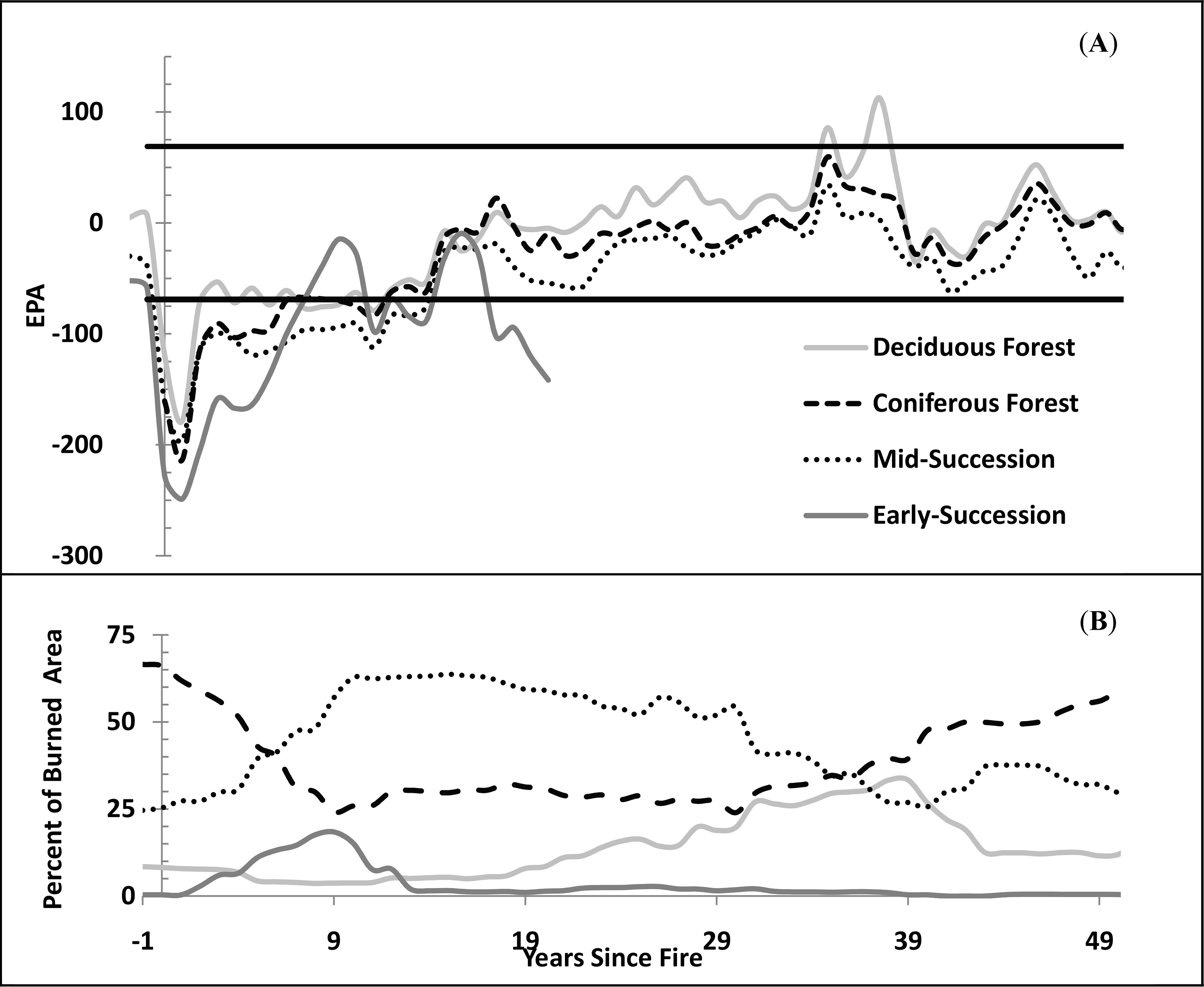
Our chronosequence demonstrated an average EPA of −33.8 (±2.1 SE), in the year prior to fire (Figure 4A), significantly lower than the overall chronosequence average EPA (−28.7 ± 0.64 SE), and the average EPA (−4.9 ± 1.1 SE) in areas that were unburned since 1950. This pattern of underperformance prior to fire may be due to reduced stand performance and photosynthetic rate at old age [91,92] or insect defoliation/mortality [4,95] inducing a negative EPA and leaving the forest more susceptible to fire. Beck and Goetz [25] found a similar pattern in a study of North American boreal forest, where a declining NDVI trend was found in the 15 years leading up to a fire. The average EPA in a fire scar in the year of burn was −158 ± 4.5 SE, which decreased to −208 ± 3.1 SE in the year immediately after the burn, and recovered to −116 ± 2.8 SE in the second year after the burn (Figure 4A). Fire often reduces performance 30%–80% in the year following a fire [43], and considerably reduces leaf area index [91], since most fires are stand replacing, resulting in severe underperformance. The lower EPA in the year after burn (as compared to the year of burn) was due to the timing of fires: a late summer fire would have smaller impacts on actual GSN in that year.
Ecosystem performance, vegetation growth, and CO2 uptake, return to pre-fire levels 5–9 years after fire [25,53]. However, average EPA in fire scars remained significantly underperforming for 10–15 years following fire, consistent with [43], and became positive 35 years following fire (Figure 4A). The interannual pattern of EPA recovery became noisier 40 years after fire due to the lower number of sample points available and the lower quality of the oldest fire perimeter data. Maximum average EPA values occurred 30–40 years after fire (Figure 4A), a finding supported by the chronosequences developed by [25] in Alaska and that of [92] in northern Manitoba, corresponding to the peak cover of deciduous species (Figure 4B). The EPA values in recovering burns during the period 30–40 years after fire tended to be higher (with an average EPA of 11.3 ± 3.2) than pre-fire conditions and compared to unburned areas, a finding consistent with that of [70]. Moreover, the EPA in deciduous stands during this period was 32 ± 5.5 (Figure 4A), significantly higher than the overall study area average of −28.7 (Table 1). Overall, the temporal recovery of average EPA following fires was best fit by a second-order polynomial relationship (R2 = 0.80, p < 0.01, y = −0.0050x2 + 7.5875x − 149.06, where y equals EPA and x equals years since fire), a relationship only valid for the first 50 years after fire.
3.4.2. Successional Patterns of Land Cover Following Fire
Boreal forest climax communities are dominated by coniferous species [29,34], occupying nearly 70% of their total area (Figure 4B). Following fire, the coniferous component markedly decreases while deciduous and herbaceous regrowth dominate, particularly in severely burned areas [15,53]. Alternatively, low intensity ground fires can occur in the organic layers [4,14]; these areas are typically self-replaced by conifers unless the soil organic layer thickness is less than 3 cm [29,52].
Early-succession, mid-succession, deciduous forest, and coniferous forest had their peak percentage of area 5, 10–15, 35, and >50 years following fire, respectively (Figure 4B). The time period 30–40 years after fire had the greatest landscape diversity (Figure 4B). Postfire vegetation is commonly deciduous stands that persist for 10–50 years following disturbance before mixing with and then gradually being replaced by coniferous stands [4,29,43,52], similar to our results. Land cover proportions of fire scar area were nearing pre-fire conditions 50 years after fire (Figure 4B), suggesting that secondary vegetation successional processes were nearly complete.
In general, yearly average EPA values following fire were positively associated with deciduous percentage of fire scar area (R2 = 0.47, p < 0.01), unrelated to coniferous and mid-successional percentage, and negatively related to early successional land cover (R2 = 0.22, p < 0.01). The successional patterns in vegetation following fire are also manifested in soils, where vegetation regrowth following fire allows for accumulation of the soil organic layer, critical to the recovery of permafrost [8] and coniferous stands. A warming temperature and changing fire frequencies could cause deviation from these successional patterns observed in our chronosequence, specifically with an increased proportion and duration of deciduous components [52].
3.5. Influence of Climate Change on Expected Ecosystem Performance
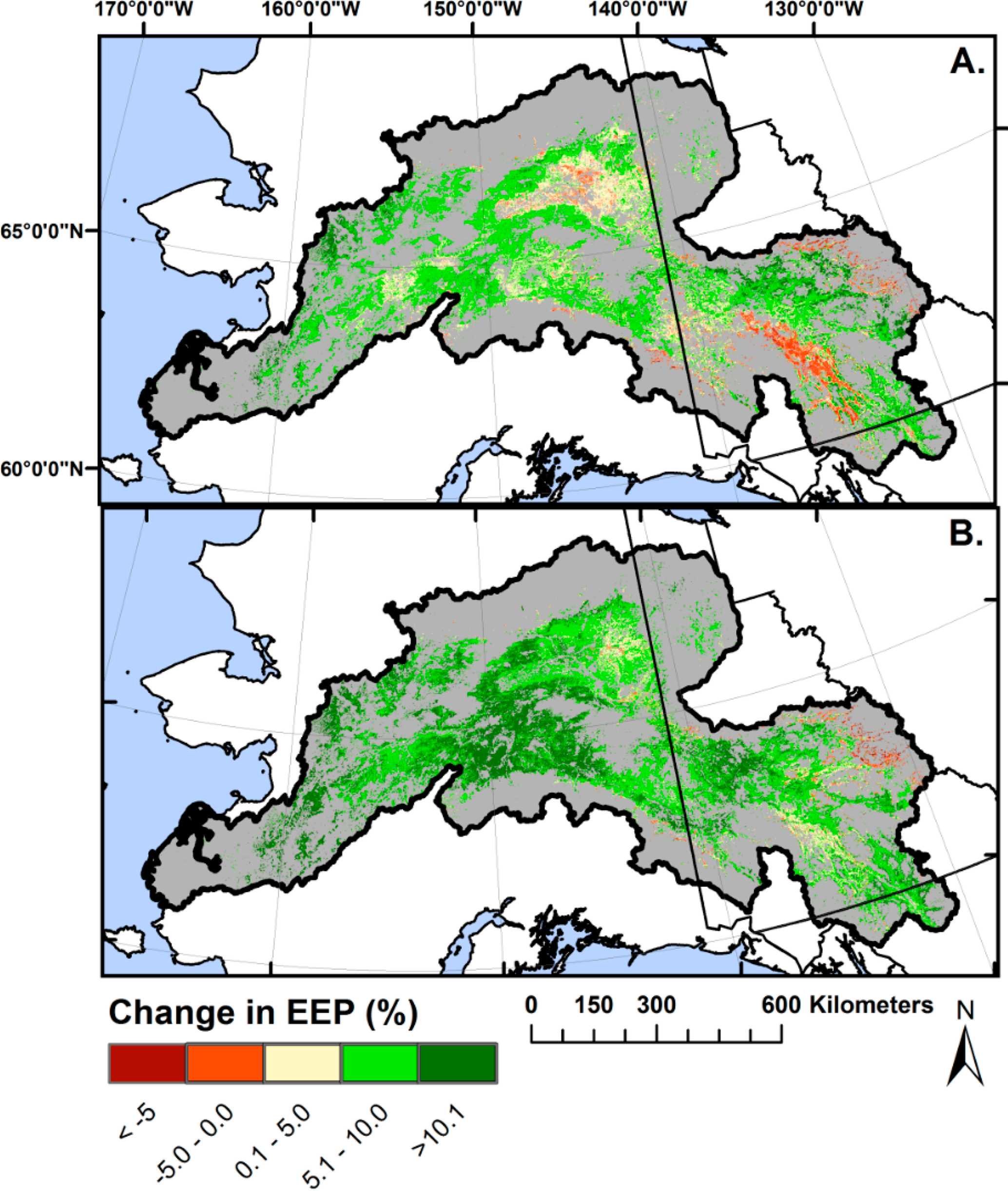
EEP model extrapolation was extremely rare when applied to future climate projections (<1% of the area). Training the EEP model on multiple years and a large number of random locations resulted in robust EEP predictions across a wide range of climatic conditions within the future climate data sets. Climate change is expected to influence mature boreal forest ecosystem performance throughout the 21st century (Figure 5). The climate projection [88] suggests a 12.4% average increase in precipitation between the 2000–2008 average and 2040, and a 23.8% increase by 2070. Under the same scenario, mean annual temperature is expected to increase by an average of 2.2 °C by 2040 and 4.1 °C by 2070 compared to the 2000–2008 baseline. The geographic patterns of warming and increased precipitation in the future are strongly related; areas with increased temperatures are also likely to be wetter (R2 > 0.80 for both periods). Our model suggests that undisturbed EEP will increase 5.6% and 8.7% in 2040 and 2070, respectively, relative to the 2000–2008 baseline.
Histograms of projected future EEP suggest that climate change will tend to broaden the range of undisturbed EEP, creating greater spatial diversity in performance. Most (92.6%) of the study area boreal forest is projected to have an increased undisturbed EEP by 2040 relative to the 2000–2008 average. Areas of decreased EEP by 2040 are concentrated in the drier portions of Yukon, Canada, and in the Yukon Flats region (Figure 5A), most of which reverse in direction to a net positive undisturbed EEP change by 2070, with 97.8% of the study area expected to have net increased undisturbed EEP by 2070. Results broadly suggest increased performance in undisturbed forests in the west and reduced to unchanged performance in the east, following precipitation contours (Figure 1), a pattern suggested by previous researchers [25,96]. Moreover, our model predicts a sharpening of the west to east performance gradient.
Declining trends in Alaska boreal forest productivity have been documented by [3,24], although large areas of no trend were also found, especially in unburned areas. Often very small, but statistically significant, declines in NDVI were documented [96]. Spruce tree ring analysis indicates declining tree growth scattered across Alaska and pan Arctic boreal forests [7,18] which may indicate opening niches for deciduous forest species advancement and increased boreal biodiversity and productivity. Conversely, more recent work in interior Alaska has demonstrated a positive correlation between black spruce tree ring growth and air temperature after the mid 1990s [97]. Increasing deciduous forest components and forest productivity in Alaska boreal forests is further supported by widespread consistent increasing trends in annual maximum NDVI on non-burned areas based on the (1982–2010) Long Term Data Record collected by the Advanced Very High Resolution Radiometer [98] and MODIS NDVI [99] and an new improved NDVI dataset with higher quality in high latitude regions (GIMMS3g) [100].
Increases in burned area and fire severity have been observed, especially in the late season, a pattern expected to continue in the future with warming [20,27], which will likely result in increased habitat availability for deciduous forest (Figure 4B). Our results of net increased ecosystem performance in the future for undisturbed forest supports the commonly reported hypothesis that the highly productive [5,16,29,33,34] deciduous component of boreal forests will increase [16,20,28,31–33], leading to further carbon uptake [30,35,36,97] and productivity increases through complementary diversity [37]. The expected shift in fire frequency and severity could result in a novel ecosystem dominated by black spruce, aspen, and birch [31], presumably increasing average EEP due to a longer successional duration and greater spatial coverage of deciduous forest. The magnitude of increased ecosystem performance increases also suggests that deciduous species may mix with stands presently dominated by less productive coniferous species in unburned areas. Additionally, since deciduous stands tend to burn less often than coniferous ones, they are more likely to reach maturity and peak performance, and provide a negative feedback to increasing fire frequency.
Due to a shorter foliar period, the duration of carbon accumulation in boreal deciduous stands is also shorter, but more intense than in coniferous stands with an average Net Ecosystem Exchange (NEE) two to three times greater than coniferous stands in June and July [36]. The GPP in both coniferous and deciduous stands in interior Alaska responded positively to spring (April–June) warming, with a 16% and 74% increase, respectively, during this portion of the growing season [36]. Late summer droughts are associated with a reduction in GPP and increase in respiration in both deciduous and coniferous stands; however, both can still serve as a net growing season carbon sink when affected by short-term severe drought (i.e., 2004) [35,36]. The impacts of longer duration droughts are less clear. Limitations with statistical model future projections (as well as some process-based models) are related to changing conditions, interactions, or feedbacks that may not be included in the model, such as increasing greenhouse gas (GHG) concentration impacts on vegetation, permafrost melting and associated potential changes of subsurface water flows [101] or terrain subsidence, emission of permafrost carbon, and future fire impacts on permafrost, carbon emission, and forest composition. These factors, feedbacks, and interactions were not explicitly included in this modeling effort and the only variable that was allowed to change for the future mapping was climate. The assumption was that the interactions that exist currently in the Yukon Basin would persist in a similar manner in the future. There are imperfections in all models and predicting the future has many unknowns and assumptions. The approach here is data-driven from a high number of observations through space and time and represents a different approach than classical mechanistic-based future predictions.
Climate change is likely to influence future species dispersal, establishment, community structure, and ecosystem performance by increasing the area and frequency of fire [3,15,22], increasing the prevalence of insect defoliation and mortality [4,95], and increasing drought-induced mortality [18,19,21]. The altered future climate may impact the resilience of stands following fire, where the regrowth may not recover to its previous coniferous dominated state [8], possibly resulting in a deciduous-dominated climax community [16,33]. This in turn may affect soil organic layer thickness and permafrost [8]. The increased deciduous forest cover in the future may also regionally serve as a negative feedback to a warming climate, since it has a higher albedo than conifer forests and an evaporative cooling effect [13,91,102]. Considering the above factors, actual net changes to ecosystem performance may differ from our results (Figure 5) due to concomitant changes in disturbance regimes and species composition [1,20,95], and these changes may be abrupt [13]. Moreover, the performance response to climate change may change or reverse after environmental thresholds have been surpassed [16].
4. Conclusions
This study produced two significant achievements. Accounting for both the effects of weather and site conditions to compare every pixel to its expected mature forest equivalent improves the utility and interpretation of time series remote sensing data by moving toward ecosystem succession and stress assessment. A data intensive (15,049 random unburned locations stratified across multiple years) regression tree model was robust to a wide range of weather and site conditions and predicted undisturbed boreal forest productivity (growing season integral of NDVI) using long-term site potential (combination of surface geology, climate, elevation, etc.) and weather (R2 = 0.53, p < 0.0001).
Our study produced two major findings. First, peak ecosystem performance and landscape diversity occurred in stands that are 30–40 years old. Second, minor increases in productivity for future undisturbed boreal forest are expected (5.6% by 2040 and 8.7% by 2070) and are anticipated to be related to an increasing deciduous forest species composition. Future projections are for mature boreal forest and do not include fire or other disturbances and further assume future Yukon River Basin boreal ecosystems will be redistribution or a subset of the current ones.
This study is unique because it provides monitoring based on deviation from what mature boreal forest productivity should be given site and weather conditions, which de-trended for interannual variations related to weather conditions and facilitated post-fire succession tracking. This study advances knowledge and informs management and field studies by identifying areas at 250 m resolution that are likely to be resilient or susceptible to change with a warming climate. This information is important to decision making related to climate implications, feedback, mitigation, and adaptation at global scales [20] and can inform land managers and users (native Alaskans) making adaptive management decisions. Future applications would be facilitated by improved input data layers including improved weather, permafrost, soil texture, and soil organic layer maps. We hope to apply this approach to identify abnormal successional paths from recent and future fires, which may reflect long-term ecosystem shifts.
Acknowledgments
This study was funded by the U.S. Geological Survey programs of LandCarbon, Climate and Land Use Research, and Development, and Climate Effects Network. We thank Lei Ji for use of their Yukon Flats biomass data and Roger Auch (USGS EROS) for reviewing an earlier version of this manuscript. The authors would like thank the Canada Centre for Remote Sensing and Environment Canada for facilitating data contributions from several federal and territorial governments, and Norman Bliss and Neal Pastick who assisted with data processing.
Author Contributions
Bruce Wylie was responsible for experimental design and theory, implementation of EPA analysis, and writing. Matthew Rigge analyzed EPA results, conducted literature research, prepared figures, and assisted with writing. Brian Brisco supported EPA analysis, provision of input layers (particularly related to Canada), and revision reviews. Kevin Murnaghan contributed analysis scripting used in EPA modeling and mapping, Canadian input layers, and version reviews. Jennifer Rover prepared input layers, constructed the merged land cover product, and organized two workshops on the analysis of the EPA data sets. Jordan Long extended the EPA analysis through the years 2007 and 2008 and edited revisions.
Conflicts of Interest
The authors declare no conflict of interest.
References
- Calef, M.P. Recent climate change impacts on the boreal forest of Alaska. Geogr. Compass 2010, 4, 67–80. [Google Scholar]
- Nemani, R.R.; Keeling, C.D.; Hashimoto, H.; Jolly, W.M.; Piper, S.C.; Tucker, C.J.; Myneni, R.B.; Running, S.W. Climate-driven increases in global terrestrial net primary production from 1982 to 1999. Science 2003, 300, 1560–1563. [Google Scholar]
- Goetz, S.J.; Bunn, A.G.; Fiske, G.J.; Houghton, R.A. Satellite-observed photosynthetic trends across boreal North America associated with climate and fire disturbance. Proc. Natl. Acad. Sci. USA 2005, 102, 13521–13525. [Google Scholar]
- McGuire, A.D.; Apps, M.; Chapin, F.S., III; Dargaville, R.; Flannigan, M.D.; Kasischke, E.S.; Kicklighter, D.; Kimball, J.; Kurz, W.; McRae, D.J.; et al. Land cover disturbances and feedbacks to the climate system in Canada and Alaska. In Land Change Science: Observing, Monitoring, and Understanding Trajectories of Change on the Earth’s Surface; Gutman, G., Janetos, A.C., Justice, C.O., Moran, E.F., Mustard, J.F., Rindfuss, R.R., Skole, D., Turner, B.L., II, Cochrane, M.A., Eds.; Kluwer Academic Publishers: Dordrecht, The Netherlands, 2004; pp. 143–165. [Google Scholar]
- Wylie, B.K.; Zhang, L.; Bliss, N.; Ji, L.; Tieszen, L.L.; Jolly, W.M. Integrating modeling and remote sensing to identify ecosystem performance anomalies in the boreal forest, Yukon River Basin, Alaska. Int. J. Digit. Earth 2008, 1, 196–220. [Google Scholar]
- Barber, V.A.; Juday, G.P.; Finney, B.P. Reduced growth of Alaskan white spruce in the twentieth century from temperature-induced drought stress. Nature 2000, 405, 668–673. [Google Scholar]
- Beck, P.S.A.; Juday, G.P.; Alix, C.; Barber, V.A.; Winslow, S.E.; Sousa, E.E.; Heiser, P.; Herriges, J.D.; Goetz, S.J. Changes in forest productivity across Alaska consistent with biome shift. Ecol. Lett 2011, 14, 373–379. [Google Scholar]
- Grosse, G.; Harden, J.; Turetsky, M.; McGuire, A.D.; Camill, P.; Tarnocai, C.; Frolking, S.; Schuur, E.A.G.; Jorgenson, T.; Marchenko, S.; et al. Vulnerability of high-latitude soil organic carbon in North America to disturbance. J. Geophys. Res. G: Biogeosci 2011, 116, G00K06:1–G00K06:23. [Google Scholar]
- Verbyla, D. The greening and browning of Alaska based on 1982–2003 satellite data. Glob. Ecol. Biogeogr 2008, 17, 547–555. [Google Scholar]
- Reed, B.C. Trend analysis of time-series phenology of North America derived from satellite data. GISci. Remote Sens 2006, 43, 24–38. [Google Scholar]
- Osterkamp, T.E. Characteristics of the recent warming permafrost in Alaska. J. Geophys. Res. F: Earth Surface 2007, 112, F02S02:1–F02S02:10. [Google Scholar]
- Hartmann, B.; Wendler, G. The significance of the 1976 Pacific climate shift in the climatology of Alaska. J. Climate 2005, 18, 4824–4839. [Google Scholar]
- Johnstone, J.F.; Chapin, F.S., III; Hollingsworth, T.N.; Mack, M.C.; Romanovsky, V.; Turetsky, M. Fire, climate change, and forest resilience in Interior Alaska1. Can. J. For. Res 2010, 40, 1302–1312. [Google Scholar]
- Ryan, K.C. Dynamic interactions between forest structure and fire behavior in boreal ecosystems. Silva Fenn 2002, 36, 13–39. [Google Scholar]
- Johnstone, J.F.; Hollingsworth, T.N.; Chapin, F.S.; Mack, M.C. Changes in fire regime break the legacy lock on successional trajectories in Alaskan boreal forest. Glob. Chang. Biol 2010, 16, 1281–1295. [Google Scholar]
- Piao, S.; Friedlingstein, P.; Ciais, P.; Zhou, L.; Chen, A. Effect of climate and CO2 changes on the greening of the Northern Hemisphere over the past two decades. Geophys. Res. Lett 2006, 33, L23402:1–L23402:6. [Google Scholar]
- Bunn, A.G.; Goetz, S.J.; Fiske, G.J. Observed and predicted responses of plant growth to climate across Canada. Geophys. Res. Lett 2005, 32, L16710:1–L16710:4. [Google Scholar]
- Lloyd, A.H.; Bunn, A.G. Responses of the circumpolar boreal forest to 20th century climate variability. Environ. Res. Lett 2007, 2, 045013:1–045013:13. [Google Scholar]
- Peng, C.; Ma, Z.; Lei, X.; Zhu, Q.; Chen, H.; Wang, W.; Liu, S.; Li, W.; Fang, X.; Zhou, X. A drought-induced pervasive increase in tree mortality across Canada’s boreal forests. Nat. Clim. Chang 2011, 1, 467–471. [Google Scholar]
- Wolken, J.M.; Hollingsworth, T.N.; Rupp, T.S.; Chapin, F.S.; Trainor, S.F.; Barrett, T.M.; Sullivan, P.F.; McGuire, A.D.; Euskirchen, E.S.; Hennon, P.E.; et al. Evidence and implications of recent and projected climate change in Alaska’s forest ecosystems. Ecosphere 2011, 2, 124:1–124:35. [Google Scholar]
- Allen, C.D.; Macalady, A.K.; Chenchouni, H.; Bachelet, D.; McDowell, N.; Vennetier, M.; Kitzberger, T.; Rigling, A.; Breshears, D.D.; Hogg, E.H.; et al. A global overview of drought and heat-induced tree mortality reveals emerging climate change risks for forests. For. Ecol. Manag 2010, 259, 660–684. [Google Scholar]
- Balshi, M.S.; McGuire, A.D.; Duffy, P.; Flannigan, M.; Kicklighter, D.W.; Melillo, J. Vulnerability of carbon storage in North American boreal forests to wildfires during the 21st century. Glob. Chang. Biol 2009, 15, 1491–1510. [Google Scholar]
- Zhang, K.; Kimball, J.S.; McDonald, K.C.; Cassano, J.J.; Running, S.W. Impacts of large-scale oscillations on pan-Arctic terrestrial net primary production. Geophys. Res. Lett 2007, 34, L21403:1–L21403:5. [Google Scholar]
- Li, S.; Potter, C. Vegetation regrowth trend in post forest fire ecosystems across North America from 2000 to 2010. Nat. Sci 2012, 4, 755–770. [Google Scholar]
- Beck, P.S.A.; Goetz, S.J. Satellite observations of high northern latitude vegetation productivity changes between 1982 and 2008: Ecological variability and regional differences. Environ. Res. Lett 2011, 6, 045501:1–045501:10. [Google Scholar]
- Yarie, J.; van Cleve, K. Long-term monitoring of climatic and nutritional affects on tree growth in Interior Alaska. Can. J. For. Res 2010, 40, 1325–1335. [Google Scholar]
- Kasischke, E.S.; Verbyla, D.L.; Rupp, T.S.; McGuire, A.D.; Murphy, K.A.; Jandt, R.; Barnes, J.L.; Hoy, E.E.; Duffy, P.A.; Calef, M.; et al. Alaska’s changing fire regime—Implications for the vulnerability of its boreal forests. Can. J. For. Res 2010, 40, 1313–1324. [Google Scholar]
- Johnstone, J.F.; Kasischke, E.S. Stand-level effects of soil burn severity on postfire regeneration in a recently burned black spruce forest. Can. J. For. Res 2005, 35, 2151–2163. [Google Scholar]
- Viereck, L.A.; Dyrness, C.T.; van Cleve, K.; Foote, M.J. Vegetation, soils, and forest productivity in selected forest types in Interior Alaska. Can. J. For. Res 1983, 13, 703–720. [Google Scholar]
- Grant, R.F.; Barr, A.G.; Black, T.A.; Margolis, H.A.; Dunn, A.L.; Metsaranta, J.; Wang, S.; McCaughey, J.H.; Bourque, C.A. Interannual variation in net ecosystem productivity of Canadian forests as affected by regional weather patterns—A Fluxnet-Canada synthesis. Agric. For. Meteorol 2009, 149, 2022–2039. [Google Scholar]
- Barrett, K.; Kasischke, E.S.; McGuire, A.D.; Turetsky, M.R.; Kane, E.S. Modeling fire severity in black spruce stands in the Alaskan boreal forest using spectral and non-spectral geospatial data. Remote Sens. Environ 2010, 114, 1494–1503. [Google Scholar]
- Lucht, W.; Schaphoff, S.; Erbrecht, T.; Heyder, U.; Cramer, W. Terrestrial vegetation redistribution and carbon balance under climate change. Carbon Balanc. Manag 2006, 1, 6:1–6:7. [Google Scholar]
- Rupp, S.T. Springsteen, A. Projected Climate Change Scenarios for the Bureau of Land Management Eastern Interior Management Area, Alaska, 2001–2099; Bureau of Land Management: Washington, DC, USA, 2009. [Google Scholar]
- Lamhamedi, M.S.; Bernier, P.Y. Ecophysiology and field performance of black spruce (Picea mariana): A review. Ann. Sci. For 1994, 51, 529–551. [Google Scholar]
- Grant, R.F.; Black, T.A.; Gaumont-Guay, D.; Klujn, N.; Barr, A.G.; Morgenstern, K.; Nesic, Z. Net ecosystem productivity of boreal aspen forests under drought and climate change: Mathematical modeling with Ecosys. Agric. For. Meteorol 2006, 140, 152–170. [Google Scholar]
- Welp, L.R.; Randerson, J.T.; Liu, H.P. The sensitivity of carbon fluxes to spring warming and summer drought depends on plant functional type in boreal forest ecosystems. Agric. For. Meteorol 2007, 147, 172–185. [Google Scholar]
- Paquette, A.; Messier, C. The effect of biodiversity on tree productivity: From temperate to boreal forests. Glob. Ecol. Biogeogr 2011, 20, 170–180. [Google Scholar]
- Tieszen, L.L.; Reed, B.C.; Bliss, N.B.; Wylie, B.K.; de Jong, D.D. NDVI, C3 and C4 production, and distributions in Great Plains grassland land cover classes. Ecol. Appl 1997, 7, 59–78. [Google Scholar]
- Gu, Y.; Wylie, B.K. Detecting ecosystem performance anomalies for land management in the upper colorado river basin using satellite observations, climate data, and ecosystem models. Remote Sens 2010, 2, 1880–1891. [Google Scholar]
- Rigge, M.; Wylie, B.; Gu, Y.; Belnap, J.; Phuyal, K.; Tieszen, L. Monitoring the status of forests and rangelands in the western United States using ecosystem performance anomalies. Int. J. Remote Sens 2013, 34, 4049–4068. [Google Scholar]
- Wylie, B.K.; Boyte, S.P.; Major, D.J. Ecosystem performance monitoring of rangelands by integrating modeling and remote sensing. Rangel. Ecol. Manag 2012, 65, 241–252. [Google Scholar]
- Chapin, F.S.; Callaghan, T.V.; Bergeron, Y.; Fukuda, M.; Johnstone, J.F.; Juday, G.; Zimov, S.A. Global change and the boreal forest: Thresholds, shifting states or gradual change? AMBIO J. Hum. Environ 2004, 33, 361–365. [Google Scholar]
- Hicke, J.A.; Asner, G.P.; Kasischke, E.S.; French, N.H.F.; Randerson, J.T.; Collatz, G.J.; Stocks, B.J.; Tucker, C.J.; Los, S.O.; Field, C.B. Postfire response of North American boreal forest net primary productivity analyzed with satellite observations. Glob. Chang. Biol 2003, 9, 1145–1157. [Google Scholar]
- Ji, L.; Wylie, B.K.; Nossov, D.R.; Peterson, B.; Waldrop, M.P.; McFarland, J.W.; Rover, J.; Hollingsworth, T.N. Estimating aboveground biomass in Interior Alaska with Landsat data and field measurements. Int. J. Appl. Earth Obs. Geoinf 2012, 18, 451–461. [Google Scholar]
- Herrmann, S.M.; Anyamba, A.; Tucker, C.J. Recent trends in vegetation dynamics in the African Sahel and their relationship to climate. Glob. Environ. Chang 2005, 15, 394–404. [Google Scholar]
- Pickup, G.; Bastin, G.N.; Chewings, V.H. Remote-sensing-based condition assessment for nonequilibrium rangelands under large-scale commercial grazing. Ecol. Appl 1994, 4, 497–517. [Google Scholar]
- Wessels, K.J.; Prince, S.D.; Carroll, M.; Malherbe, J. Relevance of rangeland degradation in semiarid northeastern South Africa to the nonequilibrium theory. Ecol. Appl 2007, 17, 815–827. [Google Scholar]
- Archer, E.R.M. Beyond the “climate versus grazing” impasse: Using remote sensing to investigate the effects of grazing system choice on vegetation cover in the eastern Karoo. J. Arid Environ 2004, 57, 381–408. [Google Scholar]
- Zurlini, G.; Petrosillo, I.; Jones, K.B.; Zaccarelli, N. Highlighting order and disorder in social-ecological landscapes to foster adaptive capacity and sustainability. Landsc. Ecol 2013, 28, 1161–1173. [Google Scholar]
- Selkowitz, D.J.; Stehman, S.V. Thematic accuracy of the National Land Cover Database (NLCD) 2001 land cover for Alaska. Remote Sens. Environ 2011, 115, 1401–1407. [Google Scholar]
- Joint Research Center Land Resource Management Unit. Available online: http://bioval.jrc.ec.europa.eu/products/glc2000/products.php (accessed on 23 September 2014).
- Barrett, K.; McGuire, A.D.; Hoy, E.E.; Kasischke, E.S. Potential shifts in dominant forest cover in Interior Alaska driven by variations in fire severity. Ecol. Appl 2011, 21, 2380–2396. [Google Scholar]
- Goulden, M.L.; Winston, G.C.; McMillan, A.M.S.; Litvak, M.E.; Read, E.L.; Rocha, A.V.; Rob Elliot, J. An eddy covariance mesonet to measure the effect of forest age on land-atmosphere exchange. Glob. Chang. Biol 2006, 12, 2146–2162. [Google Scholar]
- Jorgenson, M.T.; Racine, C.H.; Walters, J.C.; Osterkamp, T.E. Permafrost degradation and ecological changes associated with a warming climate in central Alaska. Clim. Chang 2001, 48, 551–579. [Google Scholar]
- Lu, X.; Zhuang, Q. Areal changes of land ecosystems in the Alaskan Yukon River Basin from 1984 to 2008. Environ. Res. Lett 2011, 6, 034012:1–034012:9. [Google Scholar]
- Ollinger, S.V. Sources of variability in canopy reflectance and the convergent properties of plants. New Phytol 2011, 189, 375–394. [Google Scholar]
- Barichivich, J.; Briffa, K.R.; Myneni, R.B.; Osborn, T.J.; Melvin, T.M.; Ciais, P.; Piao, S.; Tucker, C. Large-scale variations in the vegetation growing season and annual cycle of atmospheric CO2 at high northern latitudes from 1950 to 2011. Glob. Chang. Biol 2013, 19, 3167–3183. [Google Scholar]
- Huete, A.; Didan, K.; Miura, T.; Rodriguez, E.P.; Gao, X.; Ferreira, L.G. Overview of the radiometric and biophysical performance of the MODIS vegetation indices. Remote Sens. Environ 2002, 83, 195–213. [Google Scholar]
- Rigge, M.; Smart, A.; Wylie, B.; Gilmanov, T.; Johnson, P. Linking phenology and biomass productivity in South Dakota mixed-grass prairie. Rangel. Ecol. Manag 2013, 66, 579–587. [Google Scholar]
- Prince, S.D.; Tucker, C.J. Satellite remote sensing of rangelands in Botswana II. NOAA AVHRR and herbaceous vegetation. Int. J. Remote Sens 1986, 7, 1555–1570. [Google Scholar]
- Dong, J.; Kaufmann, R.K.; Myneni, R.B.; Tucker, C.J.; Kauppi, P.E.; Liski, J.; Buermann, W.; Alexeyev, V.; Hughes, M.K. Remote sensing estimates of boreal and temperate forest woody biomass: Carbon pools, sources, and sinks. Remote Sens. Environ 2003, 84, 393–410. [Google Scholar]
- Wylie, B.K.; Harrington, J.A.; Prince, S.D.; Denda, I. Satellite and ground-based pasture production assessment in Niger: 1986–1988. Int. J. Remote Sens 1991, 12, 1281–1300. [Google Scholar]
- Muukkonen, P.; Heiskanen, J. Estimating biomass for boreal forests using ASTER satellite data combined with standwise forest inventory data. Remote Sens. Environ 2005, 99, 434–447. [Google Scholar]
- Myneni, R.B.; Keeling, C.D.; Tucker, C.J.; Asrar, G.; Nemani, R.R. Increased plant growth in the northern high latitudes from 1981 to 1991. Nature 1997, 386, 698–702. [Google Scholar]
- Myneni, R.B.; Hall, F.G.; Sellers, P.J.; Marshak, A.L. Interpretation of spectral vegetation indexes. IEEE Trans. Geosci. Remote Sens 1995, 33, 481–486. [Google Scholar]
- Zhou, L.; Tucker, C.J.; Kaufmann, R.K.; Slayback, D.; Shabanov, N.V.; Myneni, R.B. Variations in northern vegetation activity inferred from satellite data of vegetation index during 1981 to 1999. J. Geophys. Res. D: Atmos 2001, 106, 20069–20083. [Google Scholar]
- Wang, J.; Rich, P.M.; Price, K.P.; Kettle, W.D. Relations between NDVI and tree productivity in the central Great Plains. Int. J. Remote Sens 2004, 25, 3127–3138. [Google Scholar]
- Jia, G.J.; Epstein, H.E.; Walker, D.A. Greening of arctic Alaska, 1981–2001. Geophys. Res. Lett 2003, 30, 2067. [Google Scholar]
- Fensholt, R.; Rasmussen, K.; Kaspersen, P.; Huber, S.; Horion, S.; Swinnen, E. Assessing land degradation/recovery in the African Sahel from long-term Earth observation based primary productivity and precipitation relationships. Remote Sens 2013, 5, 664–686. [Google Scholar]
- Tan, Z.; Liu, S.; Wylie, B.K.; Jenkerson, C.B.; Oeding, J.; Rover, J.; Young, C. MODIS-informed greenness responses to daytime land surface temperature fluctuations and wildfire disturbances in the Alaskan Yukon River Basin. Int. J. Remote Sens 2013, 34, 2187–2199. [Google Scholar]
- Fassnacht, K.S.; Gower, S.T.; MacKenzie, M.D.; Nordheim, E.V.; Lillesand, T.M. Estimating the leaf area index of North Central Wisconsin forests using the Landsat Thematic Mapper. Remote Sens. Environ 1997, 61, 229–245. [Google Scholar]
- Ji, L.; Wylie, B.; Ramachandran, B.; Jenkerson, C. A comparative analysis of three different MODIS NDVI datasets for Alaska and adjacent Canada. Can. J. Remote Sens 2010, 36, S149–S167. [Google Scholar]
- Jia, G.J.; Epstein, H.E.; Walker, D.A. Spatial heterogeneity of tundra vegetation response to recent temperature changes. Glob. Chang. Biol 2006, 12, 42–55. [Google Scholar]
- Jenkerson, C.B.; Maiersperger, T.K.; Schmidt, G.L. eMODIS: A User-Friendly Data Source; Open-File Report 2010–1055; U.S. Geological Survey: Reston, VA, USA, 2010. [Google Scholar]
- Swets, D.L.; Reed, B.C.; Rowland, J.R.; Marko, S.E. A weighted least-squares approach to temporal smoothing of NDVI. In Proceedings of the ASPRS Annual Conference, Portland, OR, USA, 17–21 May 1999.
- Khlopenkov, K.V.; Trishchenko, A.P. Implementation and evaluation of concurrent gradient search method for reprojection of MODIS level 1B imagery. IEEE Trans. Geosci. Remote Sens 2008, 46, 2016–2027. [Google Scholar]
- Luo, Y.; Trishchenko, A.P.; Khlopenkov, K.V. Developing clear-sky, cloud and cloud shadow mask for producing clear-sky composites at 250-meter spatial resolution for the seven MODIS land bands over Canada and North America. Remote Sens. Environ 2008, 112, 4167–4185. [Google Scholar]
- De’Ath, G.; Fabricius, K.E. Classification and regression trees: A powerful yet simple technique for ecological data analysis. Ecology 2000, 81, 3178–3192. [Google Scholar]
- Henderson, B.L.; Bui, E.N.; Moran, C.J.; Simon, D.A.P. Australia-wide predictions of soil properties using decision trees. Geoderma 2005, 124, 383–398. [Google Scholar]
- Howard, D.M.; Wylie, B.K. Annual crop type classification in the U.S. Great Plains for 2000–2001. Photogramm. Eng. Remote Sens 2014, 80, 537–549. [Google Scholar]
- Alaska Interagency Coordination Center. Available online: http://agdc.usgs.gov/data/blm/fire/ (accessed on 23 September 2014).
- Fulton, R.J. Surficial Materials of Canada, Map 1880A; Scale 1:5,000,000; Geological Survey of Canada: Ottawa, ON, Canada, 1995. [Google Scholar]
- National Park Service, Alaska Support Office. State Surficial Geology Map of Alaska; National Park Service, Alaska Support Office: Anchorage, AL, USA, 1999. [Google Scholar]
- Gallant, A.L.; Binnian, E.F.; Omernik, J.M.; Shasby, M.B. Ecoregions of Alaska; Professional Paper 1567; U.S. Geological Survey: Reston, VA, USA, 1995. [Google Scholar]
- Saxon, E.; Baker, B.; Hargrove, W.; Hoffman, F.; Zganjar, C. Mapping environments at risk under different global climate change scenarios. Ecol. Lett 2005, 8, 53–60. [Google Scholar]
- Brown, J.; Ferrians, O.J., Jr.; Heginbottom, J.A.; Melnikov, E.S. Circum-Arctic Map of Permafrost and Ground-Ice Conditions (Revised February 2001); U.S. Geological Survey: Boulder, CO, USA, 1998. [Google Scholar]
- McKenney, D.W.; Pedlar, J.H.; Papadopol, P.; Hutchinson, M.F. The development of 1901–2000 historical monthly climate models for Canada and the United States. Agric. For. Meteorol 2006, 138, 69–81. [Google Scholar]
- McKenney, D.W.; Price, D.; Papadapol, P.; Siltanen, M.; Lawrence, K. High-Resolution Climate Change Scenarios for North America; Frontline Technical Note No. 107; Natural Resources Canada, Great Lakes Forestry Center: Sault Ste. Marie, ON, Canada, 2006. [Google Scholar]
- Gu, Y.; Howard, D.M.; Wylie, B.K.; Zhang, L. Mapping carbon flux uncertainty and selecting optimal locations for future flux towers in the Great Plains. Landsc. Ecol 2012, 27, 319–326. [Google Scholar]
- Chen, H.Y.H.; Taylor, A.R. A test of ecological succession hypotheses using 55-year time-series data for 361 boreal forest stands. Glob. Ecol. Biogeogr 2012, 21, 441–454. [Google Scholar]
- McMillan, A.M.S.; Goulden, M.L. Age-dependent variation in the biophysical properties of boreal forests. Glob. Biogeochem. Cycles 2008, 22, GB2023:1–GB2023:14. [Google Scholar]
- Bond-Lamberty, B.; Wang, C.; Gower, S.T. Net primary production and net ecosystem production of a boreal black spruce wildfire chronosequence. Glob. Chang. Biol 2004, 10, 473–487. [Google Scholar]
- Verbyla, D.; Kasischke, E.S.; Hoy, E.E. Seasonal and topographic effects on estimating fire severity for Landsat TM/ETM+ data. Int. J. Wildland Fire 2008, 17, 527–534. [Google Scholar]
- Wylie, B.K.; Rover, J.A.; Murnaghan, K.; Long, J.B.; Tieszen, L.L.; Brisco, B. Monitoring boreal forest performance in the Yukon River Basin. In Proceedings of the Association of American Geographers, Washington, DC, USA, 12–16 April 2011.
- Baird, R.A.; Verbyla, D.; Hollingsworth, T.N. Browning of the landscape of Interior Alaska based on 1986–2009 Landsat sensor NDVI. Can. J. For. Res 2012, 42, 1371–1382. [Google Scholar]
- Parent, M.B.; Verbyla, D. The browning of Alaska’s boreal forest. Remote Sens 2010, 2, 2729–2747. [Google Scholar]
- Ueyama, M.; Kudo, S.; Iwama, C.; Nagano, H.; Kobayashi, H.; Harazono, Y.; Yoshikawa, K. Does summer warming reduce black spruce productivity in Interior Alaska? J. For. Res 2014. [Google Scholar] [CrossRef]
- Land Long Term Data Record. Available online: http://ltdr.nascom.nasa.gov (accessed on 23 September 2014).
- Budde, M. U.S. Geological Survey, Sioux Falls, SD, USA. Personal communication,. 2014. [Google Scholar]
- Guay, K.C.; Beck, P.S.A.; Berner, L.T.; Goetz, S.J.; Baccini, A.; Buermann, W. Vegetation productivity patterns at high northern latitudes: A multi-sensor satellite data assessment. Glob. Chang. Biol 2014, 20, 3147–3158. [Google Scholar]
- Walvoord, M.A.; Voss, C.I.; Wellman, T.P. Influence of permafrost distribution on groundwater flow in the context of climate-driven permafrost thaw: Example from Yukon Flats Basin, Alaska, United States. Water Resour. Res 2012, 48, W07524. [Google Scholar]
- Jin, Y.; Randerson, J.T.; Goulden, M.L.; Goetz, S.J. Post-fire changes in net shortwave radiation along a latitudinal gradient in boreal North America. Geophys. Res. Lett 2012, 39, L13403:1–L13403:7. [Google Scholar]


| Metric | 2000 | 2001 | 2002 | 2003 | 2004 | 2005 | 2006 | 2007 | 2008 | Average |
|---|---|---|---|---|---|---|---|---|---|---|
| EPA | −33.3 | −34.6 | −46.5 | −42.0 | −49.0 | −70.4 | −14.4 | 31.3 | 0.3 | −28.7 |
| EPA SE a | 0.64 | 0.55 | 0.59 | 0.60 | 0.66 | 0.76 | 0.69 | 0.69 | 0.65 | 0.64 |
| Burned (%) b | 0.8 | 0.3 | 1.2 | 0.6 | 5.2 | 3.1 | 0.2 | 0.2 | 0.1 | 1.3 |
| Insect Damage (%) b | 0.8 | 1.9 | 1.0 | 1.2 | 2.1 | 2.9 | 2.1 | 2.9 | 1.2 | 1.8 |
| Total Disturbance(%) b | 1.6 | 2.2 | 2.2 | 1.8 | 7.3 | 6.0 | 2.3 | 3.1 | 1.3 | 3.1 |
| EPA Class | ||||||||||
| Severe Under b,c | 25.0 | 21.1 | 26.7 | 24.7 | 28.4 | 35.8 | 20.2 | 11.4 | 15.8 | 18.3 |
| Under b,d | 5.4 | 6.1 | 7.4 | 6.4 | 6.6 | 6.3 | 4.0 | 2.3 | 3.7 | 5.1 |
| Low Normal b,e | 5.9 | 7.3 | 8.6 | 7.8 | 7.3 | 7.6 | 5.1 | 3.3 | 4.2 | 6.8 |
| Normal b | 50.8 | 57.3 | 50.8 | 53.4 | 49.5 | 45.3 | 49.2 | 39.4 | 50.3 | 62.2 |
| High Normal b,e | 4.0 | 3.3 | 2.6 | 2.9 | 2.9 | 2.2 | 5.3 | 6.8 | 6.4 | 3.7 |
| Over b,d | 3.0 | 2.3 | 1.8 | 1.8 | 2.0 | 1.4 | 4.0 | 6.4 | 5.0 | 2.2 |
| Highly Over b,c | 5.8 | 2.5 | 2.1 | 2.9 | 3.2 | 1.5 | 12.0 | 30.4 | 14.6 | 1.7 |
aGeographic standard error within a year;bPercent of study area;c>95% confidence departure from expected GSN;d90%–95% confidence departure from expected GSN;e80%–90% confidence departure from expected GSN.
© 2014 by the authors; licensee MDPI, Basel, Switzerland This article is an open access article distributed under the terms and conditions of the Creative Commons Attribution license (http://creativecommons.org/licenses/by/4.0/).
Share and Cite
Wylie, B.; Rigge, M.; Brisco, B.; Murnaghan, K.; Rover, J.; Long, J. Effects of Disturbance and Climate Change on Ecosystem Performance in the Yukon River Basin Boreal Forest. Remote Sens. 2014, 6, 9145-9169. https://doi.org/10.3390/rs6109145
Wylie B, Rigge M, Brisco B, Murnaghan K, Rover J, Long J. Effects of Disturbance and Climate Change on Ecosystem Performance in the Yukon River Basin Boreal Forest. Remote Sensing. 2014; 6(10):9145-9169. https://doi.org/10.3390/rs6109145
Chicago/Turabian StyleWylie, Bruce, Matthew Rigge, Brian Brisco, Kevin Murnaghan, Jennifer Rover, and Jordan Long. 2014. "Effects of Disturbance and Climate Change on Ecosystem Performance in the Yukon River Basin Boreal Forest" Remote Sensing 6, no. 10: 9145-9169. https://doi.org/10.3390/rs6109145