Sequential Method with Incremental Analysis Update to Retrieve Leaf Area Index from Time Series MODIS Reflectance Data


Abstract
: High-quality leaf area index (LAI) products retrieved from satellite observations are urgently needed for crop growth monitoring and yield estimation, land-surface process simulation and global change studies. In recent years, sequential assimilation methods have been increasingly used to retrieve LAI from time series remote-sensing data. However, the inherent characteristics of these sequential assimilation methods result in temporal discontinuities in the retrieved LAI profiles. In this study, a sequential assimilation method with incremental analysis update (IAU) was developed to jointly update model states and parameters and to retrieve temporally continuous LAI profiles from time series Moderate Resolution Imaging Spectroradiometer (MODIS) reflectance data. Based on the existing multi-year Global Land Surface Satellite (GLASS) LAI product, a dynamic model was constructed to evolve LAI anomalies over time. The sequential assimilation method with an IAU technique takes advantage of the Kalman filter (KF) technique to update model parameters, uses the ensemble Kalman filter (EnKF) technique to update LAI anomalies recursively from time series MODIS reflectance data and then calculates the temporally continuous LAI values by combining the LAI climatology data. The method was tested over eight Committee on Earth Observing Satellites-Benchmark Land Multisite Analysis and Intercomparison of Products (CEOS-BELMANIP) sites with different vegetation types. The results indicate that the sequential method with IAU can precisely reconstruct the seasonal variation patterns of LAI and that the LAI profiles derived from the sequential method with IAU are smooth and continuous.1. Introduction
Leaf area index (LAI), which is defined as one-half of the total green leaf area per unit of horizontal ground surface area [1], is an important biophysical parameter and is related to ecological processes, such as photosynthesis, respiration and transpiration. It is now widely used in climate and ecology models, including ecological system function models, crop growth models and net primary productivity models. Many methods have been developed to retrieve LAI from remote-sensing data. In general, methods to estimate LAI from satellite-sensor data can be classified into empirical methods [2,3] and physical methods [4–6]. Empirical methods are based mainly on constructing statistical relationships between LAI and a variety of vegetation indices. The main limitation of these empirical approaches is their dependence on measurement conditions, sites and vegetation types. Physical methods are based on the inversion of canopy radiative-transfer models that simulate spectral top-of-canopy bidirectional reflectance by means of physical principles and provide an explicit connection between canopy biophysical variables and the resulting canopy reflectances [7]. Because physical methods can be adjusted for a wide range of situations, an increasing number of studies tend to estimate biophysical variables using canopy radiative-transfer models. However, currently available empirical and physical methods generally use only satellite observations acquired at a specific time to retrieve LAI, which may cause temporally discontinuous and inaccurate LAI estimation. The retrieved LAI profiles exhibit many time series fluctuations, and some LAI values are missing, especially during vegetation growing seasons, because of persistent cloud cover.
To improve the quality of LAI retrievals, increasingly more attention is being paid to retrieving LAI using data assimilation techniques that are based on a reasonable consideration of the dynamic change rules of LAI and the time series satellite observations [8,9]. Currently, two types of algorithms suitable for approaching the problem of data assimilation have been developed: one is non-sequential assimilation, such as four-dimensional variational (4D-VAR) data assimilation algorithms, and the other is sequential assimilation, such as the Kalman filter (KF) and ensemble Kalman filter (EnKF) [10]. Compared with 4D-VAR data assimilation algorithms, sequential assimilation is a type of real-time assimilation system [11] and has the advantage of utilizing time series satellite observations for the real-time/near-real-time retrieval of LAI or other land surface biophysical variables. Many studies have used the sequential assimilation method to estimate real-time biogeophysical variables from satellite observations for rapid land surface change monitoring. Samain et al. [12] developed a time-evolving model based on ECOCLIMAP land cover to describe bidirectional reflectance distribution function (BRDF) seasonal evolution and used a Kalman filter to retrieve surface BRDF coefficients recursively each time that fresh observations became available. This approach ensured continuous production of surface BRDF parameters and improved the time consistency of the albedo product. Xiao et al. [13] developed a sequential assimilation method for the real-time estimation of LAI from MODIS time series reflectance data. The LAI values were updated recursively by combining predictions from dynamic models and MODIS reflectance data using an EnKF technique. The results were significantly improved over MODIS LAI when compared to field-measured LAI data. Nagarajan et al. [14] assimilated L-band microwave observations into a coupled soil-vegetation-atmosphere transfer model using an EnKF technique to improve root-zone soil moisture estimates. The assimilation method offered significant reductions in the root mean square error and the average standard deviation.
Although sequential assimilation methods can assimilate satellite observations into dynamic models sequentially during a forward integration, major drawbacks of these assimilation methods are the discontinuity between the model forecasts and the analysis estimates around the observation times and the introduced shock at the model restart stage [15–17]. This type of temporal discontinuity in the retrieved LAI profiles is inconsistent with the process of vegetation succession, during which the LAI values vary continuously with time, except in the case of disturbances (such as fires, floods and hurricanes). One method to solve this problem is called the incremental analysis update (IAU), which was first designed for assimilation systems in atmospheric circulation models to reduce initial imbalances in the model forecast [18–20]. The IAU methods incorporate analysis increments into the model hindcast in the given assimilation interval in a smooth manner [21,22] and have been widely used in atmospheric [23,24] and oceanic general-circulation models [16,20].
The LAI profiles retrieved by the sequential assimilation methods are also affected by the accuracy of the prediction from the dynamic models. In many previous studies, the dynamic models were assumed to be time-variant systems in which all quantities governing the model’s behavior remain constant with time, which affects the accuracy of the prediction from the dynamic models [13]. In fact, the dynamic models can be subject to many sources of uncertainty and are usually time-variant in the process of evolution [25]. To improve the performance of the dynamic model, an alternative approach is to develop dual state-parameter estimation methods in which the model states and parameters are estimated simultaneously from given observations [26]. In recent years, studies in many fields, such as hydrology [25,26] and aerography [27,28], have applied these dual state-parameter estimation methods to improve the forecasts of state variables.
Therefore, this paper aims at developing a sequential assimilation method with incremental analysis update to jointly update model states and parameters and retrieve temporally continuous LAI profiles from time series satellite observations. In this method, the dynamic model is used to forecast LAI based on the LAI climatology to overcome the problem of data missing. Meanwhile, the IAU method is chosen to smooth the fluctuation caused by the sequential assimilation. The assimilation method is tested using MODIS data at some flux sites and validated using ground LAI measurements.
The organization of this paper is as follows. Section 2 introduces several details of the implementation of the new assimilation method. We introduce the radiative transfer model, followed by a description about how to construct a dynamic model using an autoregressive (AR) model from Global Land Surface Satellite (GLASS) LAI time series. We then outline the techniques to update model parameters and states from time series MODIS reflectance data. Next, the IAU technique is described to smooth out discontinuities between the forecasts and the analysis estimates around the observation times. The experimental data are also described in this section. Section 3 demonstrates the performance of this new assimilation method over eight sites. Discussions are presented in Section 4, and the final section provides brief conclusions.
2. Methodology and Data
LAI climatology, defined as the average of multi-year LAI data, describes the general change tendency of LAI extracted from historical time series data. However, due to differences in temperature, precipitation and various other factors, there is always a difference between the real LAI and the LAI climatology in a given year. Let us define this difference as the LAI anomaly. In other words, the LAI anomaly represents the amount by which the real LAI is increased relative to the LAI climatology. Obviously, if the LAI anomaly is accurately known, the LAI value can be calculated on each day of the year by adding together the accurately estimated LAI anomaly and the LAI climatology. In this study, the sequential assimilation method with an IAU technique takes advantage of the KF technique to update model parameters, uses the EnKF technique to update LAI anomalies recursively from time series MODIS reflectance data and then calculates the temporally continuous LAI values by combining the LAI climatology. A flow chart outlining this method is shown in Figure 1.
The existing multi-year GLASS LAI product was used to calculate the LAI climatology and LAI anomalies. Then, a dynamic model was constructed using the LAI anomaly time series to evolve the LAI anomalies over time and was used to provide a short-range forecast of LAI anomalies. EnKF was then used to estimate the analysis of LAI anomalies by combining the predictions and the MODIS reflectance data after quality control. After this, an IAU method was developed to smooth out the discontinuities between the forecasts and the analysis estimates in the adjacent observation times. In addition, the newly obtained LAI anomaly was added to the LAI anomaly time series, and the first of the time series was dropped simultaneously. Then, the parameters of the dynamic model were updated with the new LAI anomaly time series using the KF technique before the next data-assimilation cycle to generate accurate forecasts. Detailed descriptions of the new algorithm are given in the following subsections.
2.1. Radiative-Transfer Model
The radiative-transfer model is a physical model that links canopy reflectance and canopy properties. In this study, a two-layer Analytical Canopy Reflectance Model (ACRM) developed by Kuusk [29,30] was used for canopy reflectance modelling. Table 1 lists the parameters needed to run the ACRM. Four parameters of the ACRM, which are sensitive to remote sensing data, were chosen as control variables in this study and are marked by asterisks in Table 1.
2.2. Dynamic Model
Many dynamic models have been developed to characterize the behavior of biophysical variables over time. Generally, these dynamic models can be classified into two groups: mechanical or semi-mechanical models and statistical models [26].
Mechanical or semi-mechanical models explain the course of growth on the basis of underlying physiological processes in relation to the environment [31]. Many mechanical models have been developed for different purposes [32–35]. However, most of these models have many input parameters and are driven by meteorological data. In most cases, it is hard to acquire all of these parameters accurately or the driving data at regional or global scales to run the models, which will have an impact on the accuracy of the model simulation.
Statistical models incorporate inherent change rules to evolve biophysical variables over time through statistical optimization methods. One type of commonly used statistical model, including the AR model, the linear transfer function model and the neural-network updating model, aims to predict state variables through time series analysis techniques [36]. Typically, statistical models have the advantage of short-term prediction, because of their ability to represent the relationships between input and output data flexibly. In this study, the AR model was used to describe the evolution of LAI anomalies over time based on LAI climatology.
The standard linear AR model can be described by the following equation [37]:
Although the parameters of the AR model can be determined as long as the input LAI anomaly time series is given, there is no guarantee that the model behavior will not change over time. Therefore, an adaptive AR model was used in this study to enable the model parameters to vary as the state estimates were updated.
The adaptive AR model can be described by the following equation:
2.3. Parameter Estimation of the Dynamic Model Using a Kalman Filter
After each data assimilation cycle, the parameters of the adaptive AR model were estimated. Many algorithms have been developed to estimate the time-varying parameters of adaptive AR models [38,39]. In this study, a Kalman filter [40,41] was used to estimate the time-varying parameters recursively each time a new set of LAI anomalies became available.
To use the Kalman filter to calculate the parameters of the adaptive AR model, Equation (4) can be written in the form of Equations (3) and (4):
Additionally, the analysis equation of the adaptive AR model parameters can be given by:
The superscript “a” denotes the analyzed results, and the superscript “T” denotes a matrix transpose. The one-step prediction error et is calculated as:
The remaining unknown parameters are zt and wt. Schlögl [37] summarized different methods to utilize parameters of the dynamic model to estimate zt and wt. Here, the estimation methods developed by Jazwinski [42] and Penny and Roberts [38] are used:
2.4. State Estimation of the Dynamic Model Using an Ensemble Kalman Filter
After parameter estimation of the dynamic model, a short-range forecast of LAI anomalies was provided. When observational data were available, the state estimation was conducted with the predictions from the dynamic model. In the linear case, the Kalman filter was proposed as an optimal recursive data-processing algorithm. For nonlinear problems, the extended Kalman filter (EKF) can be used after linearization of the model using a first-order Taylor series approximation. However, the EKF can lead to unstable results when the nonlinearity in the system is strong [43]. To overcome the drawbacks of EKF, Evensen [43] first proposed the EnKF as a sequential data-assimilation method to handle the nonlinearity problem.
The EnKF uses an ensemble of model states to represent the statistical errors in the model estimate and uses ensemble integrations to forecast these errors forward in time. Suppose that ξ is an n-dimension model state vector and that Y ∈ ℜn×N contains N ensemble members of the model state vector, namely Y = (ξ1, ξ2, ⋯ ξN). The ensemble mean is stored in each column of a matrix Ȳ ∈ ℜn×N, and the ensemble perturbation matrix Y′ ∈ ℜn×N is defined as Y′ = Y − Ȳ. Then, the analysis equation of EnKF for the case of linear observations is as follows:
Equation (14) imposes the condition that the measurement operator H is linear. It is invalid when the MODIS reflectance data are assimilated into a dynamic model, because the canopy reflectance model h(ξ) represents the non-linear function of the dynamic model states. This limitation can be overcome by augmenting the dynamic model state vector with a diagnostic variable, which is the model prediction of the measurement [44]. Therefore, a new model state vector can be defined as ξ̂T = [ξT, hT(ξ)], with Ŷ ∈ ℜn̂×N being the new ensemble matrix. n̂ is the sum of the size of the model state vector n and the number of measurement equivalents, and Ŷ′ ∈ ℜn̂×N is the new ensemble perturbation matrix. The new analysis equation can then be written as follows:
In this study, the model states included the variables denoted by asterisks in Table 1. Therefore, the size n of the model state vector was 4. The new ensemble matrix Ŷ combined the four variables of the model state vector and the surface reflectance for six MODIS spectral bands, meaning that n̂ was equal to 10. Measurement error covariance matrix R was defined according to the typical theoretical accuracy of six bands of MODIS reflectance data.
2.5. Incremental Analysis Updates
During the state estimation process, the predicted LAI anomalies from the adaptive AR model and the MODIS reflectance data were combined to produce the analysis of LAI anomalies using the EnKF technique. However, the inherent characteristics of sequential assimilation methods result in temporal discontinuities between the forecast and the analysis of LAI anomalies. In this study, an incremental analysis update technique was used to solve this problem.
The IAU technique incorporated analysis increments into model hindcasts and forecasts in a smooth manner [21]. Suppose that times tj−1, tj and tj+1 are three adjacent observation times, and time from tj−1 to tj+1 is defined as an assimilation interval. The prediction from the dynamic model is calculated from tj−1 to tj. At observation time tj, the EnKF is used to provide the analytical data in the way of the sequential assimilation method. At this time, the increment between the predicted result and the analysis result is computed. Then, the increment is added proportionally to the time series from tj−1 to tj+1. The dynamic model is run again from time tj−1 to tj+1, and the IAU process is repeated until the next observation time tj+1.
During IAU integration, the increment of LAI is described as the difference between the analytical result from the EnKF, , and the forecast from the dynamic model, . It is applied as shown in Equation (16):
The updated LAI anomaly is added with the LAI climatology on that day as the final result of retrieval. In addition, it is also added to the time series of LAI anomalies, and the first of the time series was dropped simultaneously. Then, the parameters of the dynamic model were updated utilizing the updated LAI anomaly time series to forecast the LAI anomaly on the next day.
2.6. Data and Preprocessing
This new assimilation method was tested over eight BELMANIP sites [45] with different biome types. The eight sites chosen were Bondville, Demmin, Utiel, Konza, Donga, the Harvard Forest, Larose and the Sonian Forest. Detailed information on these sites is shown in Table 2. The Bondville site is located in the Midwestern United States near Champaign, Illinois. This is an agricultural district with alternating years of soybean and maize crops [46]. The Demmin site is located in the Mecklenburgische Seenplatte district, Mecklenburg-Western Pomerania, Germany. The land cover is composed mainly of crops, including barley, wheat, corn, grassland, rapeseed and potatoes [47]. The Utiel site is located in the eastern part of Spain. The main land-cover type is vineyards and orchards, followed by natural Mediterranean vegetation and smaller fractions of industrial and urban areas. The topography is generally flat, with slightly hilly regions, mainly covered by natural Mediterranean vegetation [48]. The Konza site is located in the Flint Hills region of Kansas, USA. The main vegetation type here is tallgrass prairie, with small areas of gallery forest and cropland in the northern part of the study site. Donga is one of the twelve departments of Benin in West Africa. The Donga site consists of a mosaic of agricultural fields and natural vegetation, including patches of wooded savannah and gallery forests. The dominant vegetation is wooded savannah, including trees, such as Berlinia grandiflora, Daniela olivieri and Isoberlinia. The continuous herbaceous cover is made up of Andropogon, Hyparrhenia and indigo [47]. The Harvard Forest site is located in western Massachusetts, USA. It is a closed hardwood forest system with conifer and mixed hardwood-conifer areas. There are also small areas of marshy lowland, pastures and rural residential. The Larose site is located in the southeastern part of Canada. The vegetation type is forest, including boreal forest (conifers and deciduous trees) and wetland (grasses and shrubs) [47]. The Sonian Forest lies in the southeastern part of Brussels, Belgium. The land-cover type is mainly forests, such as beeches, oaks and chestnut trees. The undergrowth is sometimes very dense, including ferns and grasses [47].
At the Bondville, Konza and Harvard Forest sites, high-resolution LAI reference maps were generated from Landsat Enhanced Thematic Mapper Plus (ETM+) imagery with LAI ground measurements using the methods proposed by Gower et al. [49]. At the Demmin, Utiel, Donga, Larose and Sonian sites, LAI ground measurements were derived from hemispherical images as proposed by Lang and Yueqin [50], using SPOT images and the LAI ground measurements to calculate high-resolution LAI reference maps. To validate the accuracy of the retrieved results, the high-resolution LAI reference maps were transferred from the UTM WGS84 projection into the sinusoidal projection used in the MODIS data and were aggregated to 1-km resolution using the spatial-average method. The mean LAI reference map values for all eight sites are also given in Table 2.
The 8-day, 1-km GLASS LAI product derived from the MODIS surface reflectance data was used to calculate the LAI climatology and the LAI anomaly time series. The GLASS LAI product was retrieved using general regression neural networks, which were trained by the fused time series LAI values from MODIS and CYCLOPES LAI products and the reprocessed time series MODIS reflectance values at the BELMANIP sites [51]. The GLASS LAI product is spatially complete and temporally continuous, and the temporal smoothness of the GLASS LAI product is the best amongst the existing global LAI products [51].
For each site, the MODIS Collection 5, 8-day, 500-m land-surface reflectance product (MOD09A1) was used as the observed data to retrieve one year’s LAI profile using the new method. The specific year chosen for each site was based on available field measurements. The quality of the MODIS surface reflectance data was affected by many factors, including clouds, aerosols, water vapor and ozone. Although many of these effects were removed through atmospheric corrections, the remaining effects could sometimes be very large, requiring further processing. In this study, the contaminated reflectance data were filtered using the NDVI profile calculated from the reflectance values in the red and NIR bands and the upper envelope of the NDVI profile [13]. Only high-quality reflectance data were used to estimate LAI in this study. The MODIS reflectance data were aggregated into 1-km resolution to maintain a spatial resolution consistent with the MODIS and CYCLOPES LAI products using an average method.
3. Analysis of Results
The EnKF with IAU was used to retrieve LAI from time series MODIS reflectance data at the selected sites with different biome types. For comparison, EnKF without the IAU method was also performed over the selected sites. For better comparison and analysis of the retrieved results, both methods used the adaptive AR model with EnKF to retrieve LAI profiles from time series MODIS reflectance data. For clarification, in the following figures, the LAI values derived by the EnKF with IAU are denoted by “LAI_EnKF_IAU”, whereas the LAI values derived by the EnKF without IAU are denoted by “LAI_EnKF”. For comparison, the main-algorithm retrievals for the MODIS LAI product and the mean LAI reference map values, which are denoted by “Reference LAI”, are also shown in the following figures.
At each site, the LAI climatology was calculated from 2000 to 2010 using GLASS LAI data. The LAI anomaly time series were calculated by subtracting the LAI climatology from the GLASS LAI value. Based on the time series of LAI anomaly as the input data, an adaptive AR model was constructed to predict the LAI anomaly for the next time step. In addition, the predictions from the dynamic models and the MODIS reflectance data were combined to update the LAI using the EnKF coupled with the ACRM. Then, the discontinuities between the analysis from the EnKF and the prediction from the dynamic model were removed using the IAU technique.
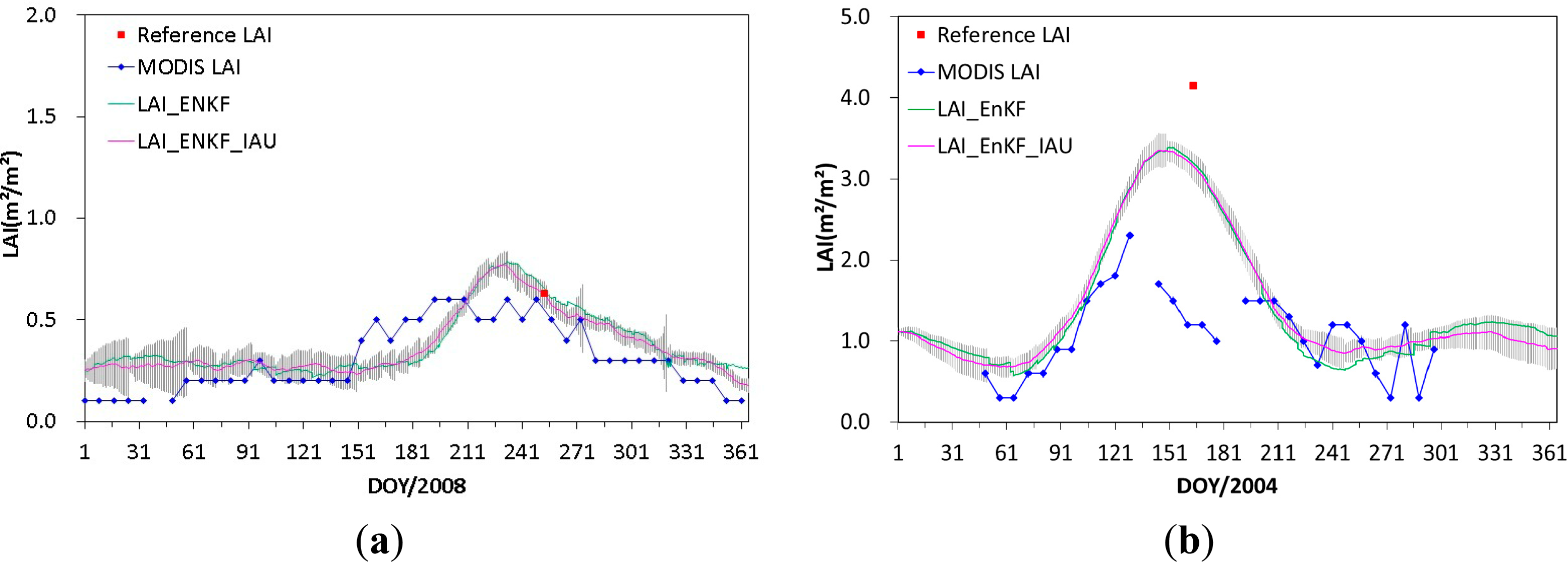
At the Utiel site (Figure 2a), the LAI anomaly time series was utilized from 2006 to 2007, providing the input data of the adaptive AR model. As seen, the LAI profile retrieved by EnKF with IAU is in agreement with the MODIS LAI profile at the beginning and the end of the crop growing season. From Day 211, the retrieved LAI values were slightly higher than the MODIS LAI values. The retrieved LAI values were closer to the reference LAI compared with the MODIS LAI at this site. By comparison with the LAI profile retrieved by EnKF without IAU, the LAI profile retrieved by EnKF with IAU tackled the discontinuities at observation times.
Figure 2b shows the retrieved results at the Demmin site in 2004. The LAI anomaly used represents 2002 to 2003. In 2004, the MODIS LAI displayed spurious temporal variations, such as sudden drops in LAI and missing data, which were possibly due to residual cloud or atmospheric effects. Good-quality observation data were chosen for the assimilation process. The LAI values retrieved by EnKF with IAU were higher than the MODIS LAI during the growing season. However, the retrieved LAI value was much closer to the reference LAI on Day 164. The difference between the retrieved LAI value and the reference LAI was 1.0, while the difference between the MODIS LAI and the reference LAI was 2.95. In the whole curve of LAI values retrieved by EnKF without IAU, unreasonable discontinuities always exist at the observation time. The IAU technique can effectively handle this type of fluctuation, which is caused by the sequential assimilation method, and make the LAI profile conform to the process of plant growth.
Figure 3a shows the LAI profiles at the Bondville site for the year 2000. Because the GLASS LAI product with 1-km resolution started in 2000, the LAI anomaly was calculated by subtracting the LAI climatology from the GLASS LAI in 2000. The retrieved results from EnKF with IAU were consistent with the MODIS LAI values before Day 210. Both the MODIS LAI values and the LAI values retrieved from EnKF with IAU were close to the reference LAI on Day 186. From Days 211 to 232, the MODIS reflectance data were missing. However, EnKF could provide reasonable LAI values through the dynamic model. On Day 224, the difference between the retrieved result and the reference LAI was 0.24. Through comparison between the LAI values retrieved from EnKF with and without IAU, spurious discontinuities existing in LAIs retrieved without IAU were removed after the application of the IAU method.
At the Konza site (Figure 3b), for the same reason as at the Bondville site, the LAI anomaly was calculated in 2000. At the beginning and end of the growing season, the curves matched well. On Day 169, the IAU results were close to the reference LAI in the absence of the MODIS LAI. From Days 185 to 240, they were slightly higher than the MODIS LAI. On Day 228, the difference between the reference LAI and the retrieved result was 0.6, while the difference between the reference LAI and the MODIS LAI was 1.1. Some stair-step jumps existed in the curve of LAI values retrieved from EnKF without IAU during the whole growing process, but when the IAU method was used, these discontinuities were removed completely.
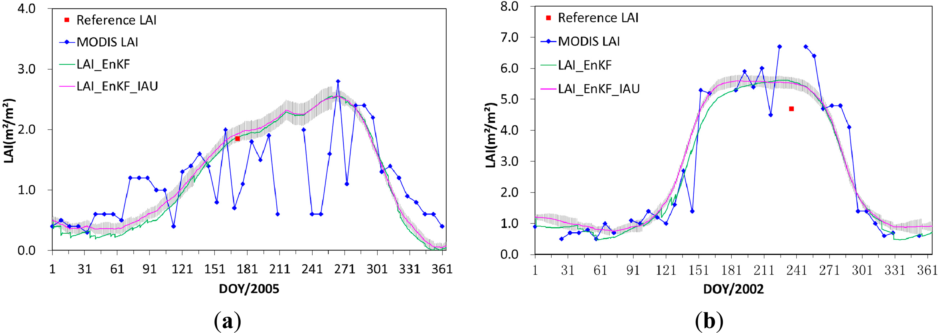
At the Donga site (Figure 4a), the LAI anomaly was calculated from 2003 to 2004. During the whole growing season, the MODIS LAI was erratic and displayed some low values, which were not realistic for this site. Excluding those observation data that exhibit poor quality, the LAI values retrieved from EnKF without IAU still exhibited large-amplitude discontinuities reproduced from the fluctuating values of the observed data, but exhibited relatively reasonable changing tendencies, especially during the peak growing season compared with the MODIS LAI. However, the IAU method damped the spurious discontinuities, included in the LAI values without IAU and presented a continuous result. The reference LAI was on Day 172. Although the MODIS LAI indicated an abrupt dip in value on that day and the difference with the reference LAI was 1.15, the IAU result still remained close to the reference, with the difference being 0.08.
Figure 4b shows the changes in LAI at the Harvard site. Because of atmospheric conditions and other reasons, there were some missing values and dramatic fluctuations in MODIS LAI. Some instability also existed in the LAI values retrieved from EnKF without IAU at the beginning of the growing season, but it was completely damped in the retrieved results from EnKF with IAU. Compared with the reference LAI on Day 236, the retrieved results from EnKF with IAU were higher, and the difference with the reference LAI was 0.82. However, because clumping and undergrowth were not taken into account in the LAI measurements at this site [52], the reference LAI here was actually an effective LAI. This indicates that some underestimation may have occurred in comparison with the true LAI values [53].
For the Larose site, the real-time retrieved LAI profile in 2003 is depicted in Figure 5a. As the input data of the adaptive AR model, the time series of LAI anomaly ran from 2001 to 2002. Only a few numbers from the MODIS LAI retrieved from the main algorithm are shown in the profile. Utilizing the assimilation with reflectance data, the retrieved results from EnKF without IAU were relatively smooth, except for a few jumps in the profile. When added to the IAU process, this method not only simulated the process of plant growth according to the dynamic model, but also updated the curve realistically according to the growth rhythm of vegetation. The reference LAI was obtained on Day 219. Although the quality of reflectance data was poor at this time, the retrieved results from EnKF with IAU still presented continuous results.
At the Sonian site (Figure 5b), the time series of the LAI anomaly was from 2002 to 2003. Dramatic fluctuations and data missing existed in MODIS LAI during the whole growing season. The retrieved LAI without IAU removed the abrupt rises and drops and provided reasonable LAI values, despite some stair-step shapes at observation times. However, the IAU method successfully handled this problem. Even though the MODIS LAI displayed unstable changes during the whole growing season, the retrieved result from EnKF with IAU was closer to the reference LAI. On Day 174, the difference between the MODIS LAI and the reference LAI was about 3.8, while the difference of the retrieved result was 0.83.
4. Discussions
A sequential assimilation method with incremental analysis updates was developed to retrieve temporally continuous LAI profiles from time series satellite observations. The method estimated states and parameters of dynamic models simultaneously from the given observations. The model behavior is adjusted after each data assimilation cycle, which leads to better characterization of the intrinsic change rules of biophysical variables. The results described in this study have shown that the adjusted dynamic model can be corrected according to the new added observation data after each data assimilation cycle.
To overcome the discontinuities between the updated LAI from the EnKF and the predicted LAI from the dynamic model, which result from the inherent characteristics of the sequential assimilation methods [13], an IAU technique was introduced to produce continuous and smooth LAI profiles that are consistent with the process of vegetation succession in this study. In fact, the ensemble Kalman smoother (EnKS) is also an effective method to smooth profiles from time series observations. It applies future observations backwards in time using the ensemble covariances [9]. However, every time a new dataset is available during the forward integration, an analysis is computed by EnKS for all previous times up to this time. Thus, the EnKS is much more CPU-intensive and also requires greater storage proportional to the total number of analysis times over which the statistics are to be applied [16]. In contrast, IAU is computationally more efficient. On the downside, the inversion method can remove abrupt spikes and dips, which may preclude a description of more local (in time) impacts of disturbances, such as fire, disease and insect damage.
In addition, the accuracy of the retrieved LAI profiles depends on the observation error and the forecast error from the dynamic model. The observation error is related to instabilities in observation, such as atmospheric, cloud contamination and calibration errors. Though quality control is used, there may still exist some errors, because the quality flags cannot ensure being absolutely right. The forecast error is mainly from the prediction process of the dynamic model. It had been shown on each day using the straight grey line. After each update, the forecast error was small, and it would gradually increase over time.
5. Conclusions
A new sequential assimilation method with IAU was developed in this study to retrieve LAI from time series MODIS reflectance data. The LAI climatology was calculated by averaging multi-year GLASS LAI data, and the LAI anomaly was obtained by subtracting the LAI climatology from the GLASS LAI value for each point in time. With the LAI anomalies as the input data, an adaptive AR model was constructed to evolve the LAI anomalies over time, and the parameters of the AR model were updated after each data assimilation cycle. The predictions from the adaptive AR model and the MODIS reflectance data were combined to update the LAI anomalies using the EnKF technique. The IAU technique was used to remove the discontinuities between the predicted LAI anomalies from the adaptive AR model and the updated LAI anomalies. The retrieved result was finally obtained from the updated LAI anomalies using the IAU technique with the added LAI climatology. The method jointly updated model states and parameters from given observations, and an IAU technique was introduced to eliminate the discontinuities between the updated LAI from the EnKF and the predicted LAI from the dynamic model. The results have demonstrated that the new method can produce temporally continuous and smooth LAI profiles from time series satellite observations. Compared with the MODIS LAI product, the retrieved LAI values are closer to the ground-based reference LAI values. In a forthcoming study, more extensive validation for all cover types will be carried out over those sites with multiple field measurements in a single year.
Acknowledgments
This work was financially supported by the Chinese 973 Program under Grant No. 2013CB733403, the Chinese 863 Program under Grant No. 2013AA12A301 and the National Natural Science Foundation of China under Grant Nos. 41171264. We would also like to thank the Committee on Earth Observation Satellites Land Product Validation (CEOS LPV) group for providing ground validation data on their website. We are grateful to the anonymous reviewers for their constructive comments.
Author Contributions
Zhiqiang Xiao conceived and designed the study. Jingyi Jiang contributed to the conception of the study, performed the data analysis and wrote the paper. Zhiqiang Xiao reviewed and edited the manuscript. All authors read and approved the manuscript.
Conflicts of Interest
The authors declare no conflict of interest.
References
- Jonckheere, I.; Fleck, S.; Nackaerts, K.; Muys, B.; Coppin, P.; Weiss, M.; Baret, F. Review of methods for in situ leaf area index determination: Part I. Theories, sensors and hemispherical photography. Agric. For. Meteorol 2004, 121, 19–35. [Google Scholar]
- Potithep, S.; Nagai, S.; Nasahara, K.N.; Muraoka, H.; Suzuki, R. Two separate periods of the LAI–VIs relationships using in situ measurements in a deciduous broadleaf forest. Agric. For. Meteorol 2013, 169, 148–155. [Google Scholar]
- Gao, S.; Niu, Z.; Huang, N.; Hou, X. Estimating the leaf area index, height and biomass of maize using HJ-1 and RADARSAT-2. Int. J. Appl. Earth Obs. Geoinf 2013, 24, 1–8. [Google Scholar]
- Koetz, B.; Baret, F.; Poilvé, H.; Hill, J. Use of coupled canopy structure dynamic and radiative transfer models to estimate biophysical canopy characteristics. Remote Sens. Environ 2005, 95, 115–124. [Google Scholar]
- Laurent, V.C.E.; Verhoef, W.; Clevers, J.G.P.W.; Schaepman, M.E. Estimating forest variables from top-of-atmosphere radiance satellite measurements using coupled radiative transfer models. Remote Sens. Environ 2011, 115, 1043–1052. [Google Scholar]
- Atzberger, C.; Richter, K. Spatially constrained inversion of radiative transfer models for improved LAI mapping from future Sentinel-2 imagery. Remote Sens. Environ 2012, 120, 208–218. [Google Scholar]
- Baret, F.; Weiss, M.; Troufleau, D.; Prevot, L.; Combal, B.; Bryson, R. Maximum information exploitation for canopy characterization by remote sensing. In Remote Sensing in Agriculture, Royal Agricultural College; Association of Applied Biologists: Cirencester, UK, 2000; pp. 71–82. [Google Scholar]
- Liang, S. Quantitative Remote Sensing of Land Surfaces, 1st ed.; John Wiley & Sons: New York, NY, USA, 2004. [Google Scholar]
- Evensen, G.; van Leeuwen, P.J. An ensemble Kalman smoother for nonlinear dynamics. Mon. Weather Rev 2000, 128, 1852–1867. [Google Scholar]
- Xiao, Z.; Wang, J.; Liang, S.; Zhou, H.; Li, X.; Zhang, L.; Jiao, Z.; Liu, Y.; Fu, Z. Variational retrieval of leaf area index from MODIS time series data: Examples from the Heihe river basin, north-west China. Int. J. Remote Sens 2012, 33, 730–745. [Google Scholar]
- European Centre for Medium-Range Weather Forecasts. Available online: http://old.ecmwf.int/ (accessed on 23 September 2014).
- Samain, O.; Roujean, J.-L.; Geiger, B. Use of a Kalman filter for the retrieval of surface BRDF coefficients with a time-evolving model based on the ECOCLIMAP land cover classification. Remote Sens. Environ 2008, 112, 1337–1346. [Google Scholar]
- Xiao, Z.; Liang, S.; Wang, J.; Jiang, B.; Li, X. Real-time retrieval of Leaf Area Index from MODIS time series data. Remote Sens. Environ 2011, 115, 97–106. [Google Scholar]
- Nagarajan, K.; Judge, J.; Monsivais-Huertero, A.; Graham, W.D. Impact of assimilating passive microwave observations on root-zone soil moisture under dynamic vegetation conditions. IEEE Trans. Geosci. Remote Sens 2012, 50, 4279–4291. [Google Scholar]
- Juckes, M.; Lawrence, B. Inferred variables in data assimilation: Quantifying sensitivity to inaccurate error statistics. Tellus A 2009, 61, 129–143. [Google Scholar]
- Lei, L.; Stauffer, D.R.; Deng, A. A hybrid nudging-ensemble Kalman filter approach to data assimilation in WRF/DART. Q. J. R. Meteorol. Soc 2012, 138, 2066–2078. [Google Scholar]
- Ourmières, Y.; Brankart, J.; Berline, L.; Brasseur, P.; Verron, J. Incremental analysis update implementation into a sequential ocean data assimilation system. J. Atmos. Ocean. Technol 2006, 23, 1729–1744. [Google Scholar]
- Bloom, S.C.; Takacs, L.L.; da Silva, A.M.; Ledvina, D. Data assimilation using incremental analysis updates. Mon. Weather Rev 1996, 124, 1256–1271. [Google Scholar]
- Carton, J.A.; Chepurin, G.; Cao, X.; Giese, B. A simple ocean data assimilation analysis of the global upper ocean 1950–95. Part I: Methodology. J. Phys. Oceanogr 2000, 30, 294–309. [Google Scholar]
- Alves, O.; Balmaseda, M.A.; Anderson, D.; Stockdale, T. Sensitivity of dynamical seasonal forecasts to ocean initial conditions. Q. J. R. Meteorol. Soc 2004, 130, 647–667. [Google Scholar]
- Benkiran, M.; Greiner, E. Impact of the incremental analysis updates on a real-time system of the North Atlantic Ocean. J. Atmos. Ocean. Technol 2008, 25, 2055–2073. [Google Scholar]
- Balmaseda, M.A.; Vidard, A.; Anderson, D.L. The ECMWF ocean analysis system: ORA-S3. Mon. Weather Rev 2008, 136, 3018–3034. [Google Scholar]
- Zhu, Y.; Todling, R.; Guo, J.; Cohn, S.E.; Navon, I.M.; Yang, Y. The GEOS-3 retrospective data assimilation system: The 6-hour lag case. Mon. Weather Rev 2003, 131, 2129–2150. [Google Scholar]
- Polavarapu, S.; Ren, S.; Clayton, A.M.; Sankey, D.; Rochon, Y. On the relationship between incremental analysis updating and incremental digital filtering. Mon. Weather Rev 2004, 132, 2495–2502. [Google Scholar]
- Gharamti, M.; Hoteit, I.; Valstar, J. Dual states estimation of a subsurface flow-transport coupled model using ensemble Kalman filtering. Adv. Water Resour 2013, 60, 75–88. [Google Scholar]
- Moradkhani, H.; Sorooshian, S.; Gupta, H.V.; Houser, P.R. Dual state–parameter estimation of hydrological models using ensemble Kalman filter. Adv. Water Resour 2005, 28, 135–147. [Google Scholar]
- Zheng, D.; Leung, J.; Lee, B. Online update of model state and parameters of a Monte Carlo atmospheric dispersion model by using ensemble Kalman filter. Atmos. Environ 2009, 43, 2005–2011. [Google Scholar]
- Hu, X.M.; Zhang, F.; Nielsen-Gammon, J.W. Ensemble-based simultaneous state and parameter estimation for treatment of mesoscale model error: A real-data study. Geophys. Res. Lett 2010, 37. [Google Scholar] [CrossRef]
- Kuusk, A. A Markov chain model of canopy reflectance. Agric. For. Meteorol 1995, 76, 221–236. [Google Scholar]
- Kuusk, A. A two-layer canopy reflectance model. J. Quant. Spectrosc. Radiat. Transf 2001, 71, 1–9. [Google Scholar]
- Spitters, C. Crop growth models: Their usefulness and limitations. In VI Symposium on the Timing of Field Production of Vegetables 267; International Society for Horticultural Science: Wageningen, The Netherlands, 1989; pp. 349–368. [Google Scholar]
- Boogaard, H.L.; van Diepen, C.A.; Rutter, R.P.; Cabrera, J.M.C.A.; Laar, H.H. User’s Guide for the WOFOST 7.1 Crop Growth Simulation Model and WOFOST Control Center 1.5; DLO Winand Staring Centre: Wageningen, The Netherlands, 1998. [Google Scholar]
- Brisson, N.; Gary, C.; Justes, E.; Roche, R.; Mary, B.; Ripoche, D.; Zimmer, D.; Sierra, J.; Bertuzzi, P.; Burger, P. An overview of the crop model STICS. Eur. J. Agron 2003, 18, 309–332. [Google Scholar]
- Jones, J.W.; Hoogenboom, G.; Porter, C.; Boote, K.; Batchelor, W.; Hunt, L.; Wilkens, P.; Singh, U.; Gijsman, A.; Ritchie, J. The DSSAT cropping system model. Eur. J. Agron 2003, 18, 235–265. [Google Scholar]
- Williams, J.; Jones, C.; Kiniry, J.; Spanel, D.A. The EPIC crop growth model. Trans. ASAE 1989, 32. [Google Scholar] [CrossRef]
- Goswami, M.; O’Connor, K.; Bhattarai, K.; Shamseldin, A. Assessing the performance of eight real-time updating models and procedures for the Brosna River. Hydrol. Earth Syst. Sci 2005, 9, 394–411. [Google Scholar]
- Schlögl, A. The Electroencephalogram and the Adaptive Autoregressive Model: Theory and Applications; Shaker Verlag GmbH: Aachen, Germany, 2000. [Google Scholar]
- Penny, W.D.; Roberts, S.J. Dynamic Linear Models, Recursive Least Squares and Steepest Descent Learning; Technical Report; Department of Electrical Engineering, Imperial College: London, UK, 1998. [Google Scholar]
- Bianchi, A.; Mainardi, L.; Meloni, C.; Chierchiu, S.; Cerutti, S. Continuous monitoring of the sympatho-vagal balance through spectral analysis. IEEE Eng. Med. Biol. Mag 1997, 16, 64–73. [Google Scholar]
- Kalman, R.E. A new approach to linear filtering and prediction problems. J. Basic Eng 1960, 82, 35–45. [Google Scholar]
- Kalman, R.E.; Bucy, R.S. New results in linear filtering and prediction theory. J. Basic Eng 1961, 83, 95–108. [Google Scholar]
- Jazwinski, A.H. Adaptive filtering. Automatica 1969, 5, 475–485. [Google Scholar]
- Evensen, G. Inverse methods and data assimilation in nonlinear ocean models. Phys. D Nonlinear Phenom 1994, 77, 108–129. [Google Scholar]
- Evensen, G. The ensemble Kalman filter: Theoretical formulation and practical implementation. Ocean Dyn 2003, 53, 343–367. [Google Scholar]
- Baret, F.; Morissette, J.T.; Fernandes, R.A.; Champeaux, J.L.; Myneni, R.B.; Chen, J.; Plummer, S.; Weiss, M.; Bacour, C.; Garrigues, S. Evaluation of the representativeness of networks of sites for the global validation and intercomparison of land biophysical products: Proposition of the CEOS-BELMANIP. IEEE Trans. Geosci. Remote Sens 2006, 44, 1794–1803. [Google Scholar]
- Meyers, T.P.; Hollinger, S.E. An assessment of storage terms in the surface energy balance of maize and soybean. Agric. For. Meteorol 2004, 125, 105–115. [Google Scholar]
- Validation of Land European Remote sensing Instruments. Available online: http://w3.avignon.inra.fr/valeri/ (accessed on 11 April 2014).
- Wigneron, J.-P.; Schwank, M.; Baeza, E.L.; Kerr, Y.; Novello, N.; Millan, C.; Moisy, C.; Richaume, P.; Mialon, A.; Al Bitar, A. First evaluation of the simultaneous SMOS and ELBARA-II observations in the Mediterranean region. Remote Sens. Environ 2012, 124, 26–37. [Google Scholar]
- Gower, S.T.; Kucharik, C.J.; Norman, J.M. Direct and indirect estimation of leaf area index, fAPAR, and net primary production of terrestrial ecosystems. Remote Sens. Environ 1999, 70, 29–51. [Google Scholar]
- Lang, A.; Xiang, Y. Estimation of leaf area index from transmission of direct sunlight in discontinuous canopies. Agric. For. Meteorol 1986, 37, 229–243. [Google Scholar]
- Xiao, Z.; Liang, S.; Wang, J.; Chen, P.; Yin, X.; Zhang, L.; Song, J. Use of general regression neural networks for generating the GLASS leaf area index product from time-series MODIS surface reflectance. IEEE Trans. Geosci. Remote Sens 2014, 52, 209–223. [Google Scholar]
- Garrigues, S.; Lacaze, R.; Baret, F.; Morisette, J.; Weiss, M.; Nickeson, J.; Fernandes, R.; Plummer, S.; Shabanov, N.; Myneni, R. Validation and intercomparison of global leaf area index products derived from remote sensing data. J. Geophys. Res 2008, 113. [Google Scholar] [CrossRef]
- Pisek, J.; Chen, J.M. Comparison and validation of MODIS and VEGETATION global LAI products over four BigFoot sites in North America. Remote Sens. Environ 2007, 109, 81–94. [Google Scholar]


| Parameter | Symbol | Value | Units |
|---|---|---|---|
| Solar zenith angle | sza | 0–90 | Degrees |
| Relative azimuth angle | raa | 0–180 | Degrees |
| Viewing zenith angle | vza | 0–90 | Degrees |
| Angstrom turbidity factor | beta | 0.1 | – |
| Ratio of leaf dimension and canopy height | rlc | 0.15 | – |
| Leaf area index * | lai | 0–10.0 | m2/m2 |
| Markov parameter * | mar | 0.4–1.0 | – |
| Factor for refraction index | fri | 0.9 | – |
| Eccentricity of the leaf angle distribution | elad | 0 | Degrees |
| Mean leaf angle of the elliptical leaf angle distribution | mla | 90 | Degrees |
| Leaf specific weight | SLW | 100 | g/m2 |
| Chlorophyll AB content | Cab | 0.4 | % of SLW |
| Leaf water content | wat | 150 | % of SLW |
| Leaf dry matter content | mat | 99.60% | % of SLW |
| Leaf structure parameter | lsp | 1.2 | – |
| Weight of the first Price function * | wpf1 | 0.05–0.4 | – |
| Weight of the second Price function * | wpf2 | −0.1–0.1 | – |
| Weight of the third Price function | wpf3 | 0 | – |
| Weight of the fourth Price function | wpf4 | 0 | – |
*Free parameters.
| Site Name | Country | Latitude (°) | Longitude (°) | Land-Cover Type | Year | DOY | Mean LAI |
|---|---|---|---|---|---|---|---|
| Utiel | Spain | 39.58 | −1.26 | Cropland | 2008 | 253 | 0.63 |
| Demmin | Germany | 53.89 | 13.21 | Cropland | 2004 | 164 | 4.15 |
| Bondville | USA | 40.004 | −88.29 | Cropland | 2000 | 186 | 2.56 |
| 2000 | 224 | 3.54 | |||||
| Konza | USA | 39.08 | −96.56 | Grassland | 2001 | 169 | 3.17 |
| 2001 | 228 | 2.9 | |||||
| Donga | Benin | 9.77 | 1.78 | Shrubs | 2005 | 172 | 1.85 |
| Harvard | USA | 42.53 | −72.17 | Mixed forest | 2002 | 236 | 4.7 |
| Larose | Canada | 45.38 | −75.21 | Mixed forest | 2003 | 219 | 5.87 |
| Sonian | Belgium | 50.77 | 4.41 | Coniferous forests | 2004 | 174 | 5.66 |
© 2014 by the authors; licensee MDPI, Basel, Switzerland This article is an open access article distributed under the terms and conditions of the Creative Commons Attribution license (http://creativecommons.org/licenses/by/4.0/).
Share and Cite
Jiang, J.; Xiao, Z.; Wang, J.; Song, J. Sequential Method with Incremental Analysis Update to Retrieve Leaf Area Index from Time Series MODIS Reflectance Data. Remote Sens. 2014, 6, 9194-9212. https://doi.org/10.3390/rs6109194
Jiang J, Xiao Z, Wang J, Song J. Sequential Method with Incremental Analysis Update to Retrieve Leaf Area Index from Time Series MODIS Reflectance Data. Remote Sensing. 2014; 6(10):9194-9212. https://doi.org/10.3390/rs6109194
Chicago/Turabian StyleJiang, Jingyi, Zhiqiang Xiao, Jindi Wang, and Jinling Song. 2014. "Sequential Method with Incremental Analysis Update to Retrieve Leaf Area Index from Time Series MODIS Reflectance Data" Remote Sensing 6, no. 10: 9194-9212. https://doi.org/10.3390/rs6109194
APA StyleJiang, J., Xiao, Z., Wang, J., & Song, J. (2014). Sequential Method with Incremental Analysis Update to Retrieve Leaf Area Index from Time Series MODIS Reflectance Data. Remote Sensing, 6(10), 9194-9212. https://doi.org/10.3390/rs6109194