Article

Combined Spectral and Spatial Modeling of Corn Yield Based on Aerial Images and Crop Surface Models Acquired with an Unmanned Aircraft System

Institute of Crop Science, University of Hohenheim, Fruwirthstr. 23, Stuttgart 70599, Germany
*
Author to whom correspondence should be addressed.
Remote Sens. 2014, 6(11), 10335-10355; https://doi.org/10.3390/rs61110335
Submission received: 19 May 2014 / Revised: 26 September 2014 / Accepted: 10 October 2014 / Published: 27 October 2014

Abstract

:
Precision Farming (PF) management strategies are commonly based on estimations of within-field yield potential, often derived from remotely-sensed products, e.g., Vegetation Index (VI) maps. These well-established means, however, lack important information, like crop height. Combinations of VI-maps and detailed 3D Crop Surface Models (CSMs) enable advanced methods for crop yield prediction. This work utilizes an Unmanned Aircraft System (UAS) to capture standard RGB imagery datasets for corn grain yield prediction at three early- to mid-season growth stages. The imagery is processed into simple VI-orthoimages for crop/non-crop classification and 3D CSMs for crop height determination at different spatial resolutions. Three linear regression models are tested on their prediction ability using site-specific (i) unclassified mean heights, (ii) crop-classified mean heights and (iii) a combination of crop-classified mean heights with according crop coverages. The models show determination coefficients R2 of up to 0.74, whereas model (iii) performs best with imagery captured at the end of stem elongation and intermediate spatial resolution (0.04 m·px1). Following these results, combined spectral and spatial modeling, based on aerial images and CSMs, proves to be a suitable method for mid-season corn yield prediction.

Graphical Abstract

1. Introduction

Corn (Zea mays L.) biomass and grain yields vary depending on site, climatic conditions and management decisions. Moreover, variation is likely to occur within fields. Following the idea of Precision Farming (PF), the identification of within-field spatial and temporal variability shows potential to support crop management concepts to meet much of the increasing environmental, economic, market and public pressures on arable agriculture [1]. Management strategies account for (i) environmental issues by adapting the input factors to the demand of the crop and, thus, avoid over- or under-application [2,3], (ii) economic issues by calculating within-field net returns [4] and (iii) possibilities to improve the control and influence of the quality of the product [5].
Yield estimations prior to harvest play a key role in the determination of input factors, like nutrients, pesticides and water, as well as for the planning of upcoming labor- and cost-intensive actions, like harvesting, drying and storage. In addition, bioenergy- and other corn-related industries benefit from these estimations, too [6]. Commonly, farmers use different methods for prediction. Coarse estimations are built on the farmer’s expert knowledge. Better estimations can be drawn from destructive sampling procedures in representative areas [7]. Unfortunately, destructive sampling is very labor-and cost-intensive work. Another approach is using yield maps, providing information about spatial and temporal variability of yields in previous years [8]. Although yield maps give some hints at within-field yield potential, they have limitations in explaining current growing conditions. Thus, reliable information about actual within-field yield estimations is usually drawn from more promising methods. Besides using linear regression models with additional information on crop management [6] or weather and soil attributes [9], several studies demonstrate the power of crop growth models to predict yield [10,11]. Although crop growth models return good estimates, their practical applicability may be limited due to the need of extensive input data for implementation. On a local and regional level, remote sensing products are quite common for estimating corn yield [12,13,14]. For a further increase in accuracy, some authors also combine actual remote sensing data and crop growth models [15,16]. Consequently, PF data has potential to improve crop development and yield prediction with smart management strategies and yield models.
With the upcoming of cheap and handy Unmanned Aircraft Systems (UASs), remotely-sensed data at high spatial and temporal resolutions have become more and more affordable [17]. Many researchers focus on RGB, multi-, hyper-spectral and thermal imaging techniques for crop monitoring [18,19,20], crop and weed discrimination [21,22] or on the generation of Digital Elevation Models (DEMs) [23,24,25,26]. Despite that, less research has been conducted on 3D Crop Surface Models (CSMs) [27,28,29] or on the possibilities of a combined analysis of both 3D and spectral information [30,31,32].
This study focuses on modeling of corn grain yield with a combined spectral and spatial analysis of aerial imagery. Standard imagery, which has been captured by a RGB consumer camera, the most common sensor used on UASs, serves as the data basis. Although RGB imagery carries limited spectral information compared to more sophisticated types, like multi-, hyper-spectral and thermal ones, its high spatial resolution allows one to create detailed CSMs for further crop investigation [28]. In addition to that, spectral information from RGB imagery can be used to determine positions of crops and estimate site-specific crop coverage factors by applying basic methods for crop/non-crop separation [33,34,35].
Recent studies found a high correlation of corn plant height and corn grain yield at early- to mid-season growth stages [36,37,38]. Yin et al. [37] also showed that linear regression models for the prediction of corn grain yield may be the preferred ones, because of their simplicity. Based on these findings, this study’s objective was to assess the potential of CSMs to predict corn grain yield at early- to mid-season growth stages by using mean crop heights and different linear regression models. The underlying hypotheses were to predict corn grain yield with simple linear regression models, building on plot-wise mean crop height as the predictor variable. The mean crop heights were generated in two ways, with and without respect to previously classified crop/non-crop pixels. Additionally, a multiple linear regression model was set up, including the crop coverage factor as a second predictor variable to improve prediction accuracy.

2. Materials and Methods

2.1. Experimental Setup

Ihinger Hof (48.74°N, 8.92°E), a research station of the University of Hohenheim, was chosen to serve as an experimental site for a field trial to predict corn grain yield by aerial imagery and crop surface models. The regional climate is categorized as a temperate climate with an annual average temperature of 7.9 °C and an average precipitation of 690 mm.
Figure 1. Overview of the two-factorial field trial in corn with 64 plots of a size of 36 × 6 m each. Four sowing densities (8–11 seeds·m2) were tested at four different levels of nitrogen fertilization (50, 100, 150 and 200 kg·N·ha1) in a setup with four replicates.
Remotesensing 06 10335 g001
A two-factorial field trial was laid out in a common randomized split-plot design on 27 May 2013, with the corn cultivar “NK Ravello”. Four sowing densities (8–11 seeds·m2) were tested at four different levels of nitrogen fertilization (50, 100, 150 and 200 kg·N·ha1) in a setup with four replicates. This resulted in 64 plots of a size of 36 × 6 m each and a total trial size of 1.38 ha (see Figure 1). Row spacing was set to 0.75 m, whereas seed spacing was adjusted according to the desired density level (0.115–0.158 m). Harvest and determination of corn grain yield with a moisture content of 14% took place on 28 October 2013, with a Global Navigation Satellite System (GNSS)-assisted combine harvester.

2.2. UAS and Sensor Setup

In this field experiment, a modified MikroKopter (MK) Hexa XL served as the aerial carrier platform to conduct sensor measurements [39]. Equipped with standard MK navigation sensors (Inertial Measurement Unit (IMU) and differential GNSS receiver), it is able to perform user-defined waypoint flights. Assembled with a payload of 1 kg and a lithium polymer battery with a capacity of 5000 mAh, this UAS operates approximately 10 min at an altitude level of 50 m above ground. With an additionally integrated Raspberry Pi Model B computer, it merges its navigation information with observations from attached sensor devices on-the-fly [40,41].
As the imaging sensor, a Canon Ixus 110 IS RGB consumer camera was attached to the UAS [42]. The camera’s sensor resolution was set to a maximum of 4000 × 3000 pixels to achieve a ground resolution of approximately 0.02 m·px1 at a flight altitude of 50 m. The camera was configured to predefined focal length (5.0 mm), aperture (f/2.8) and exposure time (1/500, 1/800 or 1/1000 s), whereas image triggering was software-controlled via a USB connection with the Raspberry Pi.

2.3. Measurements

Flight missions were performed on three dates during early- and mid-season crop development (beginning of stem elongation, end of stem elongation and end of emergence of inflorescence), referring to Zadoks’ scale’s Z32, Z39 and Z58 [43]. In each mission, aerial images were captured at a scheduled flight altitude of 50 m with an intended overlap of 80% in-track and 60% cross-track to ensure image redundancy. All images have been captured with a nadir view of direction, in clear skies and around noon. Each flight mission produced about 400 images covering all experimental plots with a ground resolution of approximately 0.02 m·px1. An overview of the flight missions is given in Table 1.
Table 1. Overview of performed flight missions at Zadoks’ scale’s crop growth stages Z32, Z39 and Z58 and the number of images for subsequent processing, flight altitude, approximate image ground resolution, mission time, illumination and wind speed.
DateGrowth StageImagesScheduled Altitude (m) Ground Resolution (m·px1)TimeIlluminationWind (m·s1)
17/07/2013Z32253500.0211–12 amclear sky1
01/08/2013Z39198500.0210–11 amclear sky2
15/08/2013Z58268500.0210–11 amclear sky2

2.4. Image Processing

Prior to processing, the selected original images were reduced in resolution to create four additional datasets of imagery at ground resolutions of 0.04, 0.06, 0.08 and 0.10 m·px1. These artificial datasets were used to simulate corn grain yield prediction performance at different spatial resolution levels of aerial imagery. Regarding the shape and structure of corn, as well as the applied plant spacing of 0.115 to 0.158 m and a row spacing of 0.75 m, the computed ground resolutions lie somewhere within the leaf and canopy level. As a consequence, high ground resolutions are expected to cover fine structures (leaf level), whereas low resolutions are expected to cover coarse structures (canopy level). The following image processing routine was performed for each dataset and crop growth stage individually.

2.4.1. Orthoimage and Digital Elevation Model

Imagery and corresponding UAS navigation information were used to generate orthoimages and DEMs with the help of the 3D reconstruction software Agisoft PhotoScan 1.0.1 [44]. In a first step of processing, all selected images were aligned, mosaicked and geo-referenced by the software’s feature matching and Structure from Motion (SfM) algorithms. In a similar way as the popular Scale-Invariant Feature Transform (SIFT) approach from Lowe [45], feature detection was performed on each image to generate descriptors for image correspondence detection. Based on the correspondences and initial GNSS image locations, the SfM algorithm reconstructed the 3D scene, camera positions and orientations [46]. In a second step, a DEM was extracted from the 3D scene by applying a natural neighbor interpolation [47]. This DEM represents the geo-referenced surface of the experimental site and is based on altitude values relative to the GNSS’ reference ellipsoid. Generally, absolute crop heights are calculated by subtracting a second DEM, a so-called Digital Terrain Model (DTM), representing the surface of the ground relative to the same reference ellipsoid as the DEM (see Figure 2).
Figure 2. Visualization of DEM and DTM altitudes relative to a commonly shared GNSS reference ellipsoid (red surface). While the DEM represents a surface model of the experimental site (green surface), the DTM represents the surface of the ground. The DTM was approximated by interpolation of ground classified DEM pixels (yellow surface). Absolute crop heights are derived by subtraction of the two surface representations.
Remotesensing 06 10335 g002
Therefore, in a third step, a DTM was inferred from the 3D scene by excluding non-ground pixels, which have been previously classified using the software’s automatic classification routine. To ensure the classification of real ground points, the point cloud was subdivided into cells of 7 × 7 m, and each cell’s lowest point was used for triangulation of a coarse initial DTM. After that, the initial DTM was densified by checking whether each remaining point meets the following two requirements: the vertical distance to the DTM-surface lies within a predefined buffer of 0.03 m, and at least one of the vectors to a ground-classified point intersects the DTM-plane with less than a predefined angle of 15°. In a last step, a mosaicked orthoimage, DEM and DTM were exported to three individual GeoTiff raster files for subsequent processing.

2.4.2. Crop Surface Model and Vegetation Indices

Further processing was performed with the statistical computation software, R [48,49,50]. The exported GeoTiff raster files were combined to a single raster stack object containing red, green, blue, DEM and DTM information as individual raster layers. A CSM raster layer was generated by pixel-wise subtraction of DTM layer altitudes from DEM layer altitudes and was added to the raster stack object.
In addition to that, three simple Vegetation Indices (VIs) were derived from the RGB bands containing the pixels’ greenness information in relation to their redness and/or blueness. The Excess Green Index (ExG), Vegetation Index Green (VIg), which is sometimes also referred to as the Normalized Green-Red Difference Index (NGRDI), and an adapted broadband variant of the Plant Pigment Ratio (PPRb) were selected as appropriate VIs to approach a detailed separation of crop and soil pixels [33,34,51,52]. Table 2 lists these VIs’ calculation formulas, which were performed on the raster stack object individually.
Table 2. Vegetation indices applied on the RGB images for pixel based crop/soil separation. The Excess Green Index (ExG) accounts for a combination of green and red, as well as green and blue reflection differences. The Vegetation Index Green (VIg) (sometimes also referred to as the Normalized Green-Red Difference Index (NGRDI)) represents a normalized green and red difference, whereas the adapted broadband variant of the Plant Pigment Ratio (PPRb) makes use of a normalized green and blue difference.
Index ReferenceExplanationFormula
ExG
Woebbecke et al. [33] & Meyer et al. [51]Excess Green Index 2 × RgreenRred Rblue
VIg
Gitelson et al. [34]Vegetation Index Green R green R red R green + R red  
PPRb
based on Metternicht [52]Plant Pigment Ratio R green R blue R green + R blue  

2.4.3. Plot-Wise Feature Extraction

Features were extracted by a self-developed automatic routine. First, field trial plot information was imported as a polygonal shapefile. For this analysis, plot size was reduced to rectangles of 9 × 6 m around the original plots’ centers to account for plot boundary effects, e.g., sowing or fertilization inaccuracies. Second, a shapefile containing harvested corn yield information was imported, and mean corn yields were determined for each individual plot. Third, mean plot heights were calculated using height information from the CSM layer. Fourth, for each VI layer, all pixels that fall inside a plot were extracted, and five different thresholds were computed on the selected pixels’ aggregated histogram based on the method of Ridler and Calvard [53] and Kort [50]. Consequently, VI layer pixels were classified as non-crop pixels in the case that the pixels’ values were below the defined thresholds and as crop pixels in the case that they were above the defined thresholds, respectively (see Figure 3).
Figure 3. VI-based Ridler thresholding by the example of a 4 × 4 m sub-sample of plot 413 with a sowing density of 11 seeds·m2 and nitrogen application of 50 kg·N·ha1. The upper left corner shows the RGB orthoimage, which is displayed at a ground resolution of 0.04 m and at crop growth stage Z39. The second image in the upper row shows the ExG layer, which was derived from the RGB orthoimage. Based on the ExG layer’s histogram, five different thresholds were computed. Threshold r3 is the original Ridler threshold, whereas the other thresholds represent four variations on the Ridler method (upper right corner). The remaining images show the ExG layer’s classification (green = crop, yellow = soil) based on the five thresholds. In this example, threshold r3 and r4 seem to classify best. Thresholds r1 and r2 seem to overestimate crop coverage, while r5 seems to underestimate crop coverage.
Remotesensing 06 10335 g003
Fifth, for each VI layer and its five identified thresholds, mean plot heights were calculated using the CSM layer height information solely from crop-classified pixels (see Figure 4). Sixth, for each VI layer and its five identified thresholds, plot crop coverage was computed by dividing the number of crop-classified pixels by the total number of pixels in each plot.
Figure 4. Mean crop height computation using the example of a 4 × 4 m sub-sample of plot 413 with a sowing density of 11 seeds·m2 and nitrogen application of 50 kg·N·ha1. The lower part of the figure shows a stack of the RGB orthoimage and the ExG layer classification based on threshold r4 at a ground resolution of 0.04 m and at crop growth stage Z39. The upper part shows the corresponding CSM layer height information as a 3D representation, colored by the ExG-classification. Mean crop height was calculated by the crop-classified CSM layer heights only and is displayed as a semi-transparent plane.
Remotesensing 06 10335 g004

2.5. Modeling Strategy

In the last step of processing, the extracted features were used to model corn grain yield with three different strategies. Based on the findings of Yin et al. [37] that all investigated regression models predict sufficiently well, standard linear regression models were set up for prediction. Assuming that Yiis the harvested corn grain yield, Hirs is the i-th mean plot height, regardless of any pixel classification, at the r-th ground resolution level and the s-th growth stage, whereas b0 and b1 are the regression coefficients. Equation (1) shows a simple linear regression model for corn grain yield prediction, forming strategy S1.
Y i = ( b 0 + b 1 × H ¯ i r s ) + ε i r s
Strategy S2 was laid out in the same way as strategy S1, except Hirstv representing the i-th mean plot height calculated from pixels, which were classified as crop by using the v-th VI layer and the t-th Ridler threshold estimate at the r-th ground resolution and s-th growth stage (Equation (2)).
Y i = ( b 0 + b 1 × H ¯ i r s t v ) + ε i r s t v
The third strategy S3 is a multiple linear regression approach, extending strategy S2. This approach accounts for a second predictor variable Cirstvrepresenting the i-th plot crop coverage factor, which was computed by the v-th VI layer, and the t-th Ridler threshold estimate at the r-th ground resolution and the s-th growth stage (Equation (3)).
Y i = ( b 0 + b 1 × H ¯ i r s t v + b 2 × C i r s t v ) + ε i r s t v
While the first two strategies follow the approach of Yin et al. [37], strategy S3 also considers the crop coverage factor as an additional predictor for expected corn grain yield.

2.6. Statistical Analysis

Statistical analysis was conducted with the statistical computation software, R. The field trial was analyzed as a mixed model using a standard two-way analysis of variance (ANOVA) approach. All modeling strategies for corn grain yield prediction were tested with and without classification-based mean crop heights at all crop growth stages, ground resolutions, Ridler threshold estimates and deduced crop coverage factors. The prediction accuracy of the different modeling strategies was assessed by using R2 determination coefficient values as quality indicators. Spatial visualization of predicted and harvested corn grain yield was carried out using the geographical information system QGIS [54].

3. Results and Discussion

3.1. Field Trial

The ANOVA showed a significant influence of nitrogen fertilization on corn grain yield. Significant influences of sowing density, as well as of the interaction of both factors were not detected. The non-significant influence of sowing density was not expected, but might have been caused by the small variability in the range of sowing density levels of 8–11 seeds·m2. Detailed results are not presented in the following.

3.2. Image Processing

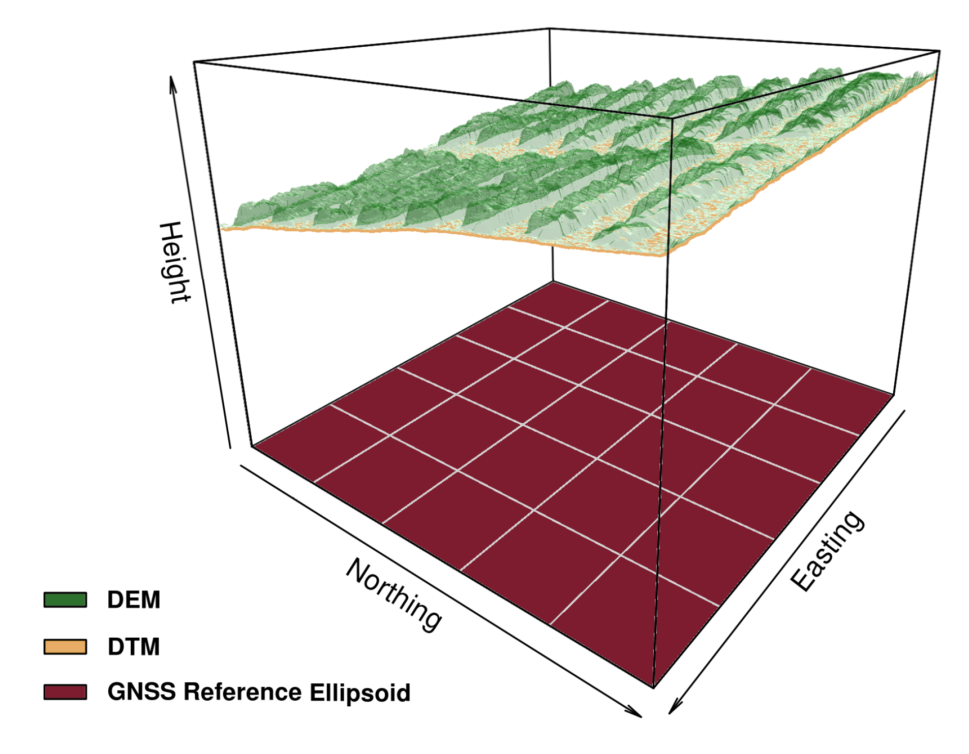
The 3D reconstruction software, Agisoft PhotoScan 1.0.1, was able to perform image alignment and 3D scene reconstruction for all imagery datasets. Geo-referencing was based on camera location information, derived from GNSS and IMU data. Orthoimage, DEM and DTM computation succeeded for all imagery datasets. Resulting orthoimage ground resolution was at the level of input image ground resolution. As dense point cloud reconstruction is a very hardware-demanding task, the imagery used for DEM and DTM generation was downscaled by a factor of two to save processing time. Although DEM and DTM were exported with the corresponding orthophoto’s ground resolution, the underlying dense point cloud was built with less detail than theoretically possible.
As the produced DTMs are based on the interpolation of previously classified ground points, this method is generally prone to misclassification at dense crop stands and canopy closure. In these situations, only a small amount of ground points will be visible at all, weakening the reliability of the interpolation results. Moreover, some of the classified points may not represent the “real” ground, leading to an underestimation of crop heights. In a homogeneous field, a correction factor could compensate for this underestimation. In an inhomogeneous field, the correction factor would not be constant anymore. To avoid these problems, it is recommended to produce DTMs at sowing stage, without the need for classification and interpolation of large gaps.
Geo-referencing accuracy was assessed by the help of 24 Ground Control Points (GCPs), which were installed permanently and measured with RTK-GNSS equipment. Heavy rainfalls in July silted many of the GCPs. In addition, others have been destroyed by intensive mechanical weed control in between the corn strips. Unfortunately, the GCPs were not renewed before performing flight missions at Z39 and Z58. As a consequence, imagery from these stages lack accurate GCP information. Thus, accuracy assessment was performed on Z32 imagery, only.
Table 3. Resulting root mean squared errors (m) (RMSE) at ground control point (GCP) locations for indirectly (GCP-based) and directly (GNSS- and IMU-based) geo-referenced imagery at Z32 for all image ground resolutions.
Geo-ReferenceCoordinate ComponentGround Resolution (m·px1)
0.020.040.060.080.10
GCPsHorizontal0.0580.0630.0840.0890.082
Vertical0.0680.0590.0510.0460.075
GNSS & IMUHorizontal0.4300.3750.3990.4090.376
Vertical0.3030.2730.2830.3200.379
In addition to direct (GNSS- and IMU-based) geo-referencing, indirect (GCP-based) geo-referencing was conducted on Z32 imagery for enhanced CSM quality assessment. Table 3 lists the resulting root mean squared errors of a comparison of measured and computed GCP coordinates for both methods and all image ground resolutions at Z32. As expected, indirectly geo-referenced imagery showed smaller residuals than the directly geo-referenced one. Horizontal RMSEs for indirectly geo-referenced imagery ranged from 0.058 to 0.089 m, whereas vertical RMSEs ranged from 0.046 to 0.075 m. In contrast to that, horizontal RMSEs for directly geo-referenced imagery ranged from 0.375 to 0.430 m, whereas vertical RMSEs ranged from 0.273 to 0.379 m. The accuracies of both methods are in accordance with the findings of Turner et al. [55] and Ruiz et al. [56], although vertical accuracy performs slightly better than expected. GCP-based accuracy assessment for directly geo-referenced imagery at Z39 and Z58 was not performed. Nevertheless, comparison of identifiable field boundaries with those of Z32 did not show excessive horizontal accuracy errors for all resolutions.
The developed R-routine managed to calculate CSMs, VIs and all threshold variants for every imagery dataset. CSM quality was assessed by comparison of mean plot heights at Z32, derived from accurate and indirectly geo-referenced imagery, with those derived from less accurate and directly geo-referenced imagery. Table 4 shows the resulting root mean squared errors for plot height comparisons, ranging from 0.024 m for high resolution imagery to 0.008 m for low resolution imagery. With a difference of 0.20 m in between the highest and lowest mean plot height at Z32, direct geo-referencing shows little influence on mean plot height computation. Unfortunately, independent reference measurements, e.g., manual height measurements, 3D laser scanning datasets or CSMs, derived by other SfM software packages, were not available to assess absolute CSM accuracy. Therefore, subsequent analyses and results are proven for this dataset, only.
Table 4. Resulting root mean squared errors (m) (RMSE) of comparing mean plot heights calculated from indirectly (GCP-based) and directly (GNSS- and IMU-based) geo-referenced imagery at Z32 for all image ground resolutions.
ValueCoordinate ComponentGround Resolution (m·px1)
0.020.040.060.080.10
Plot HeightVertical0.0240.0100.0090.0100.008
Horizontal alignment errors of directly geo-referenced imagery strongly influence the results of automatic feature extraction. To account for misalignment, the polygonal shapefile, containing this field trial’s plot information, was realigned individually for all imagery at all growth stages and image ground resolutions.
The computed original Ridler thresholds r3 were regarded as suitable for automatic separation of crop and soil, as well as most of the threshold variants r2 and r4. In contrast to that, threshold variants r1 and r5 showed results of crop overestimation at threshold r1 and underestimation at threshold r5, respectively (see e.g., Figure 3). However, mean plot heights Hirstv and crop coverage factors Cirstv were computed for all strategies at every threshold level r15 for subsequent comparison of prediction performance.

3.3. Modeling Strategy

All results of the applied corn grain yield prediction strategies are summarized in Table 5, whereas Figure 5 visualizes the most important findings. Strategy S3 was evaluated for collinearity of its predictor variables, mean crop height and crop coverage. Critical collinearity at any crop growth stage was not found. As all strategies built on data from one growing period, leave-one-out cross-validation was conducted to evaluate each model’s predictive quality. Table 6 shows the resulting root mean squared errors of prediction (RMSEP), ranging from 0.67 to 1.28 t·ha1 (8.8% to 16.9%).
Crop growth stage Z32 was neglected in Figure 5, as none of the strategies resulted in R2 determination coefficient values higher than 0.56. As crops were still small and stems were beginning to elongate, crops’ leaves were not overlapping at this point in time. Lacking canopy closure, the prediction models had to account for information contained at the leaf level. Therefore, imagery with highest resolutions of 0.02 and 0.04 m·px1 performed best and showed significant R2 values. In contrast, lower resolution datasets did not provide much detail, resulting in low R2 values. Strategy S3 was generally able to significantly improve prediction accuracies of strategies S1 and S2 for all VIs by adding the crop coverage factor as the second predictor variable. Although the highest resolution imagery of 0.02 m·px1 performed best at this stage, even higher resolutions may be more appropriate for CSM and, thus, mean plot height generation. Reaching maximum R2 values of 0.56 and considering additional environmental impacts on crop growth during the growing season, none of the applied strategies was assessed to be reliable for early-season corn grain yield prediction.
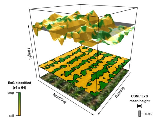
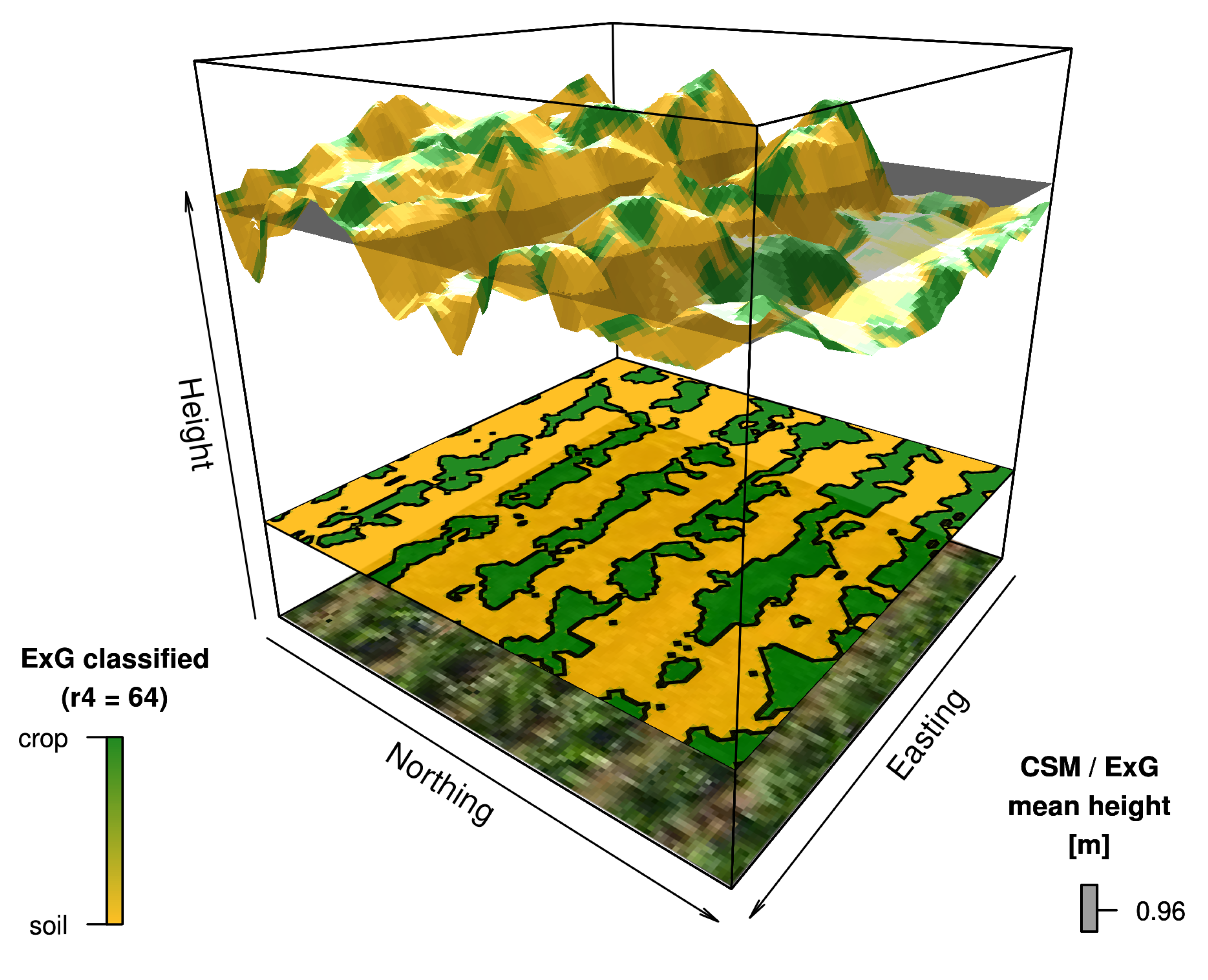
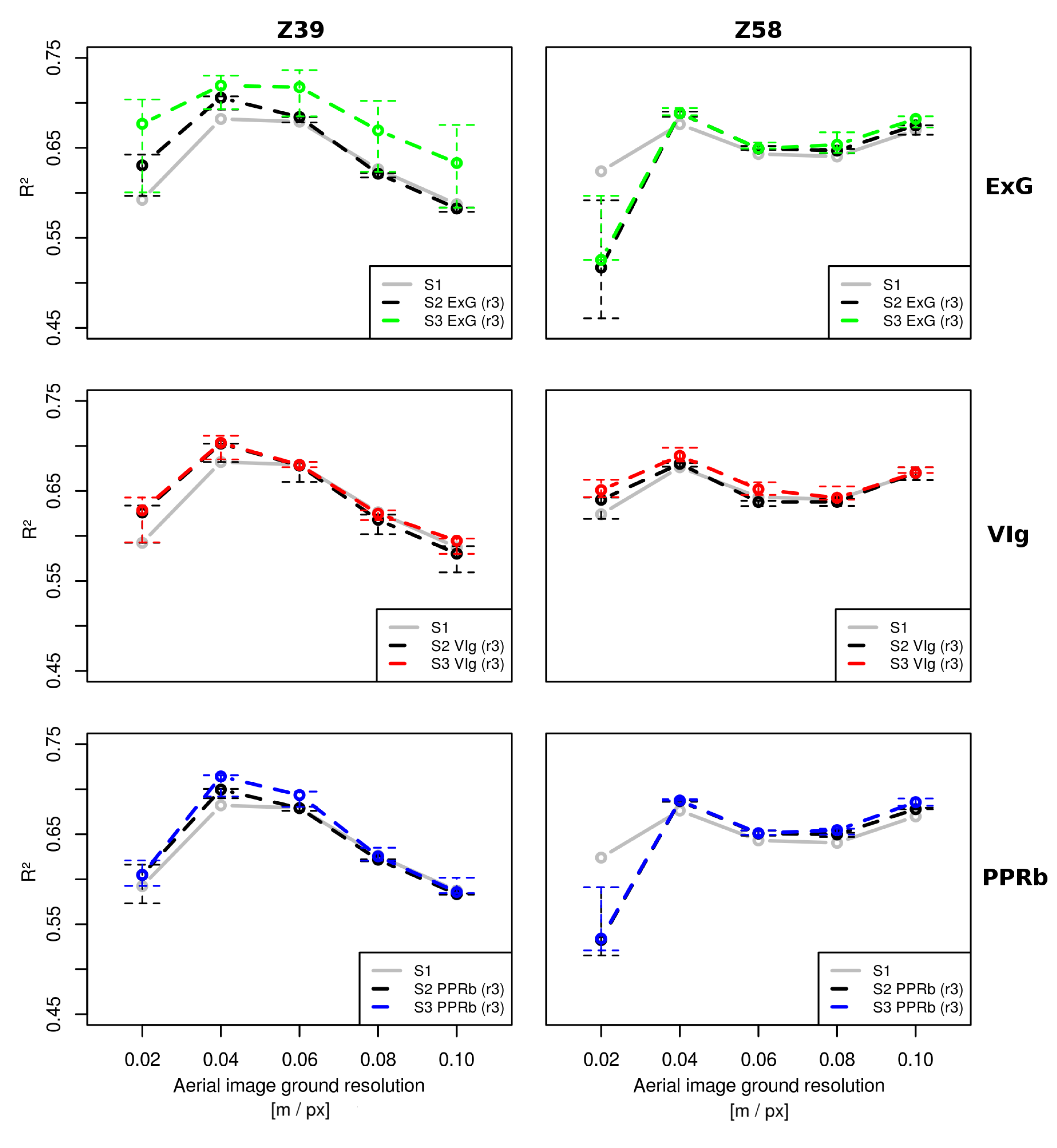
Figure 5. Resulting determination coefficients R2 of modeling strategies S3 for all VIs and aerial image ground resolutions at crop growth stages Z39 and Z58. Grey values represent R2 values for strategy S1, whereas black values represent strategy S2 at Ridler threshold r3 and colored values represent strategy S3 at Ridler threshold r3, respectively. In addition to the R2 values of strategies S2 and S3 at Ridler threshold r3, minimum and maximum R2 values of the four remaining threshold variants are indicated as range bars for every aerial image ground resolution individually.
Remotesensing 06 10335 g005
Table 5. The resulting determination coefficients R2 of the prediction of corn grain yield by applying strategies S13 for all combinations of VIs, aerial image ground resolutions, crop growth stages and computed Ridler thresholds. Significance codes for predictor variable crop height are represented as *in superscript, whereas significance codes for predictor variable crop coverage factor are represented as *in subscript (appearing only in strategy S3).
Ground Res. (m·px−1)ExGVIgPPRb
ZSxrx0.020.040.060.080.100.020.040.060.080.100.020.040.060.080.10
Z32S1 0.48***0.26***0.12**0.050.09*0.48***0.26***0.12**0.050.09*0.48***0.26***0.12**0.050.09*
Z32S2 r10.54***0.27***0.12**0.050.09*0.53***0.25***0.11**0.050.08*0.46***0.25***0.11**0.050.09*
Z32S2 r20.55***0.24***0.11**0.040.08*0.55***0.21***0.09*0.030.07*0.47***0.21***0.080.030.08*
Z32S2 r30.55***0.23***0.08*0.030.08*0.46***0.16***0.050.020.050.46***0.18***0.050.020.07*
Z32S2 r40.53***0.20***0.06*0.020.06*0.36***0.11**0.020.010.040.42***0.14**0.030.010.04
Z32S2 r50.51***0.17***0.040.010.050.25***0.09*0.010.010.050.37***0.09*0.020.000.03
Z32S3 r1 0.54***0.30*0.21*0.20**0.21**0.53***0.25* 0.130.070.10 0.52 * * * * * 0.30 * * 0.19*0.13*0.18*
Z32S3 r2 0.55*** 0.36 * * * 0.32***0.31***0.33***0.56*** 0.31 * * * 0.23**0.19***0.21** 0.53 * * * * * 0.35 * * * * 0.27***0.23***0.27***
Z32S3 r3 0.55*** 0.38 * * * * 0.35***0.34***0.38*** 0.52 * * * * * 0.37 * * * * 0.32***0.31***0.34*** 0.52 * * * * * 0.37 *** * 0.33***0.30***0.33***
Z32S3 r4 0.55*** 0.37 * * * * 0.33***0.32***0.38*** 0.47 * * * * * * 0.35 * * * * 0.31***0.32***0.37*** 0.50 * * * * * 0.36 *** * 0.32***0.30***0.33***
Z32S3 r5 0.52*** 0.33 * * * * 0.29***0.29***0.34*** 0.41 * * * * * * 0.31 * * * * 0.28***0.29***0.36*** 0.46 * * * * * 0.33 *** * 0.30***0.29***0.32***
Z39S1 0.59***0.68***0.68***0.63***0.59***0.59***0.68***0.68***0.63***0.59***0.59***0.68***0.68***0.63***0.59***
Z39S2 r1 0.60***0.69***0.68***0.62***0.58***0.59***0.68***0.68***0.62***0.59***0.57***0.69***0.68***0.62***0.58***
Z39S2 r2 0.62***0.70***0.68***0.62***0.58***0.61***0.70***0.68***0.62***0.58***0.59***0.70***0.68***0.62***0.58***
Z39S2 r3 0.63***0.71***0.68***0.62***0.58***0.63***0.70***0.68***0.62***0.58***0.60***0.70***0.68***0.62***0.58***
Z39S2 r4 0.64***0.71***0.68***0.62***0.58***0.63***0.70***0.67***0.61***0.57***0.61***0.70***0.68***0.62***0.58***
Z39S2 r5 0.64***0.71***0.68***0.62***0.58***0.63***0.70***0.66***0.60***0.56***0.62***0.70***0.68***0.62***0.58***
Z39S3 r1 0.60***0.69***0.69***0.62***0.58***0.59***0.68***0.68***0.63***0.60***0.59***0.69***0.68***0.63***0.60***
Z39S3 r2 0.65 * * * * 0.71***0.70***0.64***0.60***0.62***0.70***0.68***0.63***0.59***0.59***0.71***0.69***0.62***0.58***
Z39S3 r3 0.68 * * * * * 0.72*** 0.72 * * * * * 0.67 * * * * * 0.63 * * * * * 0.63***0.70***0.68***0.62***0.59***0.60***0.71***0.69***0.63***0.59***
Z39S3 r4 0.69 * * * * * 0.73 * * * * 0.73 * * * * * 0.69 * * * * * * 0.66 * * * * * * 0.64***0.71***0.68***0.62***0.59***0.61***0.72***0.70***0.63***0.59***
Z39S3 r5 0.70 * * * * * * 0.73 * * * * 0.74 * * * * * * 0.70 * * * * * * 0.68 * * * * * * 0.64***0.71***0.68***0.62***0.58***0.62***0.71*** 0.70 * *** 0.64***0.60***
Z58S1 0.62***0.68***0.64***0.64***0.67***0.62***0.68***0.64***0.64***0.67***0.62***0.68***0.64***0.64***0.67***
Z58S2 r1 0.59***0.68***0.65***0.64***0.67***0.64***0.68***0.64***0.64***0.68***0.59***0.69***0.65***0.65***0.68***
Z58S2 r2 0.55***0.69***0.65***0.65***0.67***0.64***0.68***0.64***0.64***0.67***0.56***0.69***0.65***0.65***0.68***
Z58S2 r3 0.52***0.69***0.65***0.65***0.68***0.64***0.68***0.64***0.64***0.67***0.53***0.69***0.65***0.65***0.68***
Z58S2 r4 0.49***0.69***0.65***0.65***0.67***0.63***0.68***0.64***0.64***0.67***0.52***0.69***0.65***0.65***0.68***
Z58S2 r5 0.46***0.69***0.65***0.65***0.66***0.62***0.68***0.63***0.63***0.66***0.52***0.69***0.65***0.65***0.68***
Z58S3 r1 0.60***0.69***0.65***0.64***0.67***0.64***0.68***0.65***0.64***0.68***0.59***0.69***0.65***0.65***0.69***
Z58S3 r2 0.55***0.69***0.65***0.65***0.68***0.65***0.68***0.65***0.64***0.67***0.56***0.69***0.65***0.66***0.69***
Z58S3 r3 0.53***0.69***0.65***0.65***0.68***0.65***0.69***0.65***0.64***0.67***0.53***0.69***0.65***0.65***0.69***
Z58S3 r4 0.53 * * * *   0.69***0.65***0.66***0.69*** 0.66 * * * *   0.69***0.66***0.65***0.67***0.52***0.69***0.65***0.65***0.68***
Z58S3 r5 0.54 * * * * *   0.69***0.66***0.67***0.68*** 0.66 * * * * *   0.70 * * * *   0.66 * * * *   0.65***0.67***0.52***0.69***0.65***0.65***0.68***
Significance Codes R2H(sig.height)R2C(sig.coverage)***: p< 0.001 **: p< 0.01 *: p< 0.05
Z39 was identified as the crop growth stage with the best prediction performance. Figure 5 points out the most interesting findings. Generally, all VIs performed well, although the best results were achieved using ExG. High and intermediate ground resolutions of 0.04 and 0.06 m·px1 showed R2 values of up to 0.74 for strategy S3. However, strategy S3 improved results for ExG only. VIg and PPRb did not show significant improvements. Strategy S2 outperformed strategy S1 for resolutions of 0.02 and 0.04 m·px1, whereas at intermediate and low ground resolutions, strategies S1 and S2 did not differ in prediction accuracy. Coarse VI layer information and the beginning of canopy closure seemed to level out differences of simple plot mean height computation and the classification-based one. Unexpectedly, the highest resolution of 0.02 m·px1 performed worse than high/intermediate resolutions. Although strategies S2 and S3 significantly improved prediction using ExG, highest resolution strategies appeared to be prone to higher noise and a scale effect, as the level of resolution leads to analysis in between leaf and canopy level. As a consequence, CSM and classification results may be biased.
Table 6. The resulting root mean squared errors of prediction (RMSEP) of the leave-one-out cross-validation for evaluation of the predictive quality of applying strategies S13 for all combinations of VIs, aerial image ground resolutions, crop growth stages and computed Ridler thresholds.
Ground Res. (m·px1)ExGVIgPPRb
ZSxrx0.020.040.060.080.100.020.040.060.080.100.020.040.060.080.10
Z32S1 0.931.111.201.251.210.931.111.201.251.210.931.111.201.251.21
Z32S2r10.881.111.211.251.210.891.131.211.251.220.941.121.211.251.21
Z32S2r20.861.131.211.251.220.871.151.221.261.230.931.141.221.251.22
Z32S2r30.871.141.231.261.220.951.171.241.261.240.941.161.241.261.23
Z32S2r40.881.151.241.261.231.031.201.261.271.240.981.191.261.271.24
Z32S2r50.901.171.251.271.241.111.221.271.271.241.021.211.271.281.26
Z32S3r10.901.101.161.171.150.901.141.231.261.230.911.101.191.231.19
Z32S3r20.881.041.071.081.060.871.081.141.161.150.911.071.131.161.13
Z32S3r30.881.021.051.051.020.901.031.071.081.050.911.041.081.101.07
Z32S3r40.881.031.061.071.030.951.051.081.071.030.931.041.081.091.07
Z32S3r50.901.071.101.091.061.001.081.101.091.040.961.071.091.101.07
Z39S1 0.830.730.740.790.830.830.730.740.790.830.830.730.740.790.83
Z39S2r10.830.710.730.800.830.830.730.740.800.830.850.720.740.800.83
Z39S2r20.800.700.730.800.830.810.700.740.800.830.830.710.740.800.83
Z39S2r30.790.700.730.800.830.790.700.740.800.840.810.700.740.800.83
Z39S2r40.780.690.730.800.840.780.700.750.810.850.810.700.740.800.83
Z39S2r50.770.690.740.800.840.780.700.760.820.860.800.700.740.800.83
Z39S3r10.840.720.740.810.850.840.730.740.800.830.840.730.750.800.83
Z39S3r20.780.710.730.790.830.810.710.750.810.840.840.700.740.810.85
Z39S3r30.750.690.700.760.790.800.710.760.810.840.830.690.730.800.84
Z39S3r40.730.680.680.730.760.790.700.750.810.840.810.690.730.800.83
Z39S3r50.710.670.680.720.740.780.700.750.810.850.810.700.730.790.83
Z58S1 0.820.720.770.770.740.820.720.770.770.740.820.720.770.770.74
Z58S2r10.850.720.760.760.730.790.720.770.770.730.850.710.760.760.73
Z58S2r20.890.710.760.760.730.790.720.770.770.730.890.710.760.760.73
Z58S2r30.930.710.760.760.730.800.720.770.770.740.910.710.760.760.73
Z58S2r40.960.710.760.760.730.800.720.780.770.740.930.710.760.760.73
Z58S2r50.980.710.760.760.740.820.720.780.770.750.930.720.760.760.73
Z58S3r10.850.720.770.770.740.800.730.780.780.740.860.720.770.760.72
Z58S3r20.900.720.770.770.740.800.730.780.780.740.900.720.770.760.72
Z58S3r30.940.720.770.760.730.790.720.770.780.740.920.720.770.760.73
Z58S3r40.930.720.770.750.730.780.710.760.770.740.930.720.770.760.73
Z58S3r50.920.720.760.750.730.780.710.760.760.740.930.720.770.770.73
At Z58, results were strongly influenced by the occurrence of canopy closure. Hence, neither strategy S2 nor strategy S3 were able to significantly improve the corn grain yield prediction performance of strategy S1. Moreover, highest resolution strategies showed similar patterns as in Z39. Except using VIg, imagery at a ground resolution of 0.02 m·px1 seemed to underlay CSM and misclassification as in Z39. All other resolutions performed comparatively well, independent of applied strategy and VI. Although, these resolutions did not reach the maximum R2 values of Z39, they were still considered as suitable for prediction.
Figure 6. 
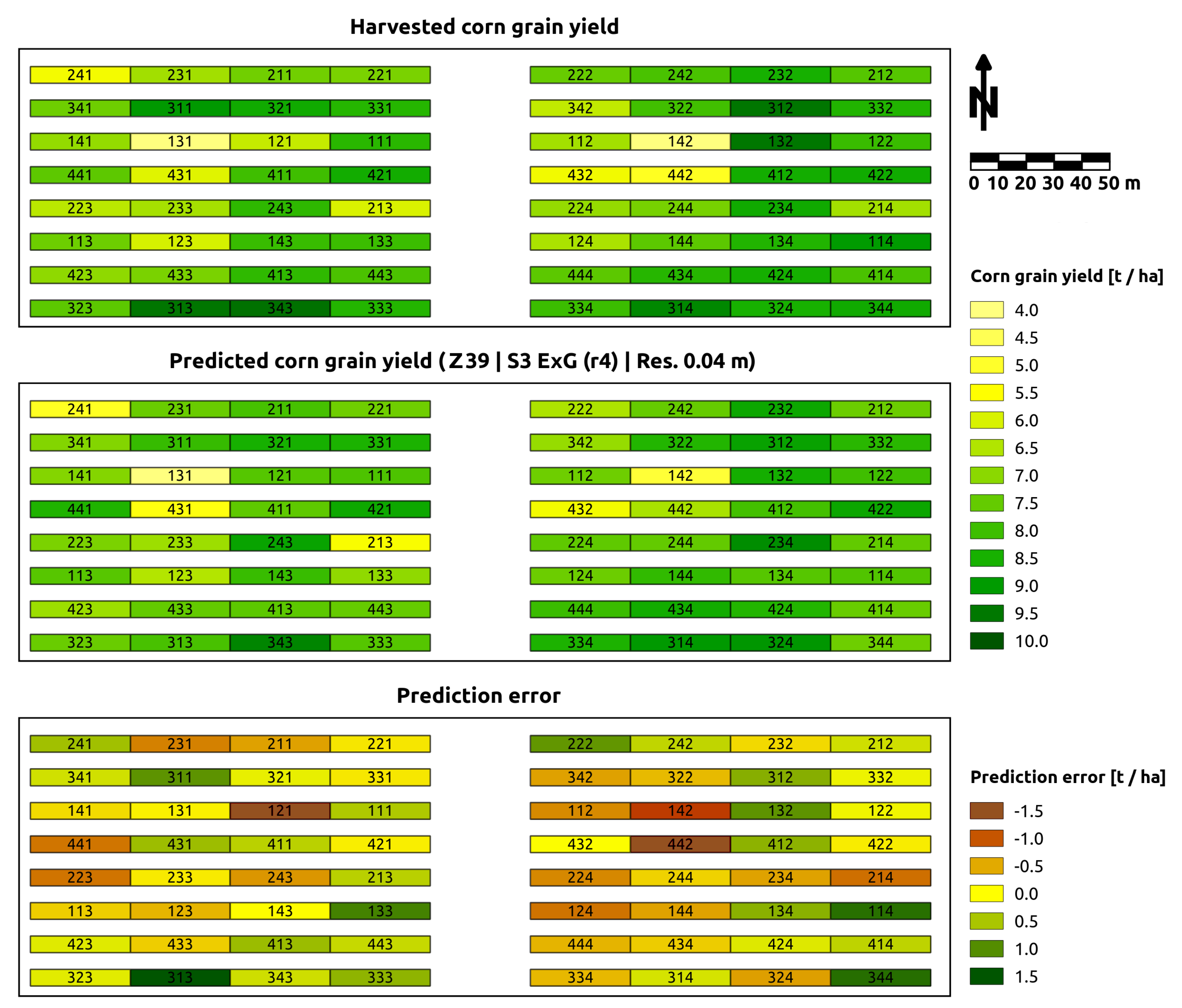
Spatial illustration of plot-wise distribution of harvested corn grain yield (top), corn grain yield predicted by strategy S3 at crop growth stage Z39, with ExG at Ridler threshold r4 and an aerial image ground resolution of 0.04 m·px1 (middle) and the resulting prediction error of this strategy (bottom). For this strategy, the total root mean squared error of prediction (RMSEP) equals 0.68 t·ha1 (8.8%).
Remotesensing 06 10335 g006
Table 7 summarizes the key findings. The most suitable resolution and modeling strategy depends on the crop growth stage. Due to row-based cultivation of corn and missing canopy closure, early growth stages require very high resolution imagery for accurate CSM computation and classification-based separation of crop and soil. Therefore, strategies S2 and S3 result in higher R2 values than strategy S1 (R2 ≤ 0.56). With ongoing crop development and beginning canopy closure, high resolution imagery and crop/soil classification gets less and less important. Highest resolution imagery showed a significant reduction of prediction accuracy at mid-season growth stages. All other imagery resolutions performed almost equally well (approximately 0.60 ≤ R2 ≤ 0.70) at all strategies S13 within these stages. Best prediction results were achieved by applying strategy S2 and especially strategy S3 at Z39 (R2 ≤ 0.74). Although strategy S3 proved to have good performance at this specific growth stage, further investigation of the influence of crop coverage factor Cirstv on the prediction results of this multiple linear regression strategy seems of great interest.
Table 7. Overview of the best performing parameters for early- to mid-season corn grain yield prediction at different crop growth stages. So far, the increase in prediction performance in strategy S3 appears to underlay an unknown factor. Therefore, strategy S3 is listed in brackets.
Growth Stage
Z32Z39Z58
Ground Resolution highest/highhigh/intermediatehigh/intermediate/low
Vegetation Index ExGExGVIg
Prediction Strategy S2 / (S3)S2 / (S3)S1 / S2 / (S3)
These findings indicate the best corn grain yield prediction at mid-season crop growth stages Z39 and Z58. They are in accordance with the findings of Yin et al. [37]. Nevertheless, none of the strategies showed results comparable to the best predictions of Yin et al. [37]. Depending on the growth stage and crop rotation system, Yin et al. [37] stated significant determination coefficients of 0.25 ≤ R2 ≤ 0.89, whereas low R2 values were achieved at early-season growth stages, only.
Applying strategy S3 at Z39, Figure 6 visualizes plot-wise prediction results and compares them to the harvested corn grain yield. Using ExG at Ridler threshold r4 and an aerial image ground resolution of 0.04 m·px−1, the total RMSEP equals 0.68 t·ha1 (8.8%). Although this strategy performed best, the ANOVA of the field trial’s input factors did not show significant influence of sowing density on corn grain yield. As strategy S3 utilizes computed crop coverage Cirstvas the estimator for sowing/stand density, the increase in prediction performance seems to underlay another factor, correlated with Cirstv. Other combinations of strategy S3 and VIg/PPRb did not show improved results compared to strategy S2.

4. Conclusions

This work shows the potential of exploiting spectral and spatial information from UAS-based RGB imagery for predicting corn grain yield in early- to mid-season crop growth stages. RGB imagery was used to compute crop surface models and to extract crop height information. In combination with RGB-based VI information, three different linear regression models were tested for the prediction of corn grain yield with R2 determination coefficients of up to 0.74 and RMSEP ranging from 0.67 to 1.28 t·ha1 (8.8% to 16.9%).
Generally, all tested VIs performed almost equally well at any crop growth stage. The same applies to tested classification thresholds r24. Although some of the more extreme thresholds r1 and r5 showed satisfying results, these thresholds cannot be recommended, because of potential over- or under-estimation of crop coverage.
The most suitable resolution and modeling strategy depends on the crop growth stage. Due to row-based cultivation of corn and missing canopy closure, early growth stages require very high resolution imagery for accurate CSM computation and classification-based separation of crop and soil. Compared to using simple unclassified mean crop heights (S1), prediction results significantly improve, when accounting for additional crop/soil classification information (S2 and S3). With ongoing crop development and beginning canopy closure, high resolution imagery gets less and less important, sometimes even disadvantageous, due to higher noise. Good prediction results are achieved at intermediate resolutions by considering crop coverage as the second predictor variable (S3). With the completion of canopy closure, neither high resolution imagery nor crop/soil classification show potential to further improve prediction. Concluding these findings, combined spectral and spatial modeling, based on aerial images and CSMs, proves to be a suitable method for mid-season corn yield prediction.

Acknowledgments

The authors acknowledge the Carl-Zeiss Foundation (Carl-Zeiss-Stiftung) for funding this work as part of the collaborative project “SenGIS” at the University of Hohenheim, Stuttgart, Germany.

Author Contributions

Jakob Geipel performed the field work, acquired the data, processed the imagery into VI layers and CSMs, computed the Ridler thresholds and mean crop heights, set up the corn yield predicition models, and wrote the manuscript. Johanna Link proposed the field trial’s design, supported the statistical analysis, and wrote the introduction. Wilhelm Claupein proposed the idea for this study and helped with editorial contributions.

Conflicts of Interest

The authors declare no conflicts of interest.

References

  1. Stafford, J. Implementing precision agriculture in the 21st century. J. Agr. Eng. Res. 2000, 76, 267–275. [Google Scholar] [CrossRef]
  2. Delin, S. Site-Specific Nitrogen Fertilization Demand in Relation to Plant Available Soil Nitrogen and Water. PhD Thesis, Swedish University of Agricultural Sciences, Skara, Sweden, 2005. [Google Scholar]
  3. Flowers, M.; Weisz, R.; White, J. Yield-based management zones and grid sampling strategies: Describing soil test and nutrient variability. Agron. J. 2005, 97, 968–982. [Google Scholar] [CrossRef]
  4. Link, J.; Graeff, S.; Batchelor, W.D.; Claupein, W. Evaluating the economic and environmental impact of environmental compensation payment policy under uniform and variable-rate nitrogen management. Agric. Syst. 2006, 91, 135–153. [Google Scholar] [CrossRef]
  5. Bongiovanni, R.G.; Robledo, C.W.; Lambert, D.M. Economics of site-specific nitrogen management for protein content in wheat. Comput. Electron. Agric. 2007, 58, 13–24. [Google Scholar] [CrossRef]
  6. Mourtzinis, S.; Arriaga, F.J.; Balkcom, K.S.; Ortiz, B.V. Corn grain and stover yield prediction at R1 growth stage. Agron. J. 2013, 105, 1045–1050. [Google Scholar] [CrossRef]
  7. Lauer, J. Methods for Calculating Corn Yield. http://corn.agronomy.wisc.edu/AA/pdfs/A033.pdf (accessed on 3 July 2014).
  8. Blackmore, S. The interpretation of trends from multiple yield maps. Comput. Electron. Agric. 2000, 26, 37–51. [Google Scholar] [CrossRef]
  9. Rodrigues, M.S.; Cora, J.E.; Castrignano, A.; Mueller, T.G.; Rienzi, E. A spatial and temporal prediction model of corn grain yield as a function of soil attributes. Agron. J. 2013, 105, 1878–1887. [Google Scholar] [CrossRef]
  10. Thorp, K.R.; DeJonge, K.C.; Kaleita, A.L.; Batchelor, W.D.; Paz, J.O. Methodology for the use of DSSAT models for precision agriculture decision support. Comput. Electron. Agric. 2008, 64, 276–285. [Google Scholar] [CrossRef]
  11. Batchelor, W.D.; Basso, B.; Paz, J.O. Examples of strategies to analyze spatial and temporal yield variability using crop models. Eur. J. Agron. 2002, 18, 141–158. [Google Scholar] [CrossRef]
  12. Aparicio, N.; Villegas, D.; Casadesus, J.; Araus, J.L.; Royo, C. Spectral vegetation indices as nondestructive tools for determining durum wheat yield. Agron. J. 2000, 92, 83–91. [Google Scholar] [CrossRef]
  13. Pinter, P.J.; Jackson, R.D.; Idso, S.B.; Reginato, R.J. Multidate spectral reflectance as predictors of yield in water stressed wheat and barley. Int. J. Remote Sens. 1981, 2, 43–48. [Google Scholar] [CrossRef]
  14. Salazar, L.; Kogan, F.; Roytman, L. Using vegetation health indices and partial least squares method for estimation of corn yield. Int. J. Remote Sens. 2008, 29, 175–189. [Google Scholar] [CrossRef]
  15. Wang, J.; Li, X.; Lu, L.; Fang, F. Estimating near future regional corn yields by integrating multi-source observations into a crop growth model. Eur. J. Agron. 2013, 49, 126–140. [Google Scholar] [CrossRef]
  16. Fang, H.; Liang, S.; Hoogenboom, G.; Teasdale, J.; Cavigelli, M. Corn-yield estimation through assimilation of remotely sensed data into the CSM-CERES-Maize model. Int. J. Remote Sens. 2008, 29, 3011–3032. [Google Scholar] [CrossRef]
  17. Van der Wal, T.; Abma, B.; Viguria, A.; Previnaire, E.; Zarco-Tejada, P.; Serruys, P.; van Valkengoed, E.; van der Voet, P. Fieldcopter: Unmanned aerial systems for crop monitoring services. In Precision Agriculture ’13; Stafford, J., Ed.; Wageningen Academic Publishers: Wageningen, The Netherlands, 2013; pp. 169–175. [Google Scholar]
  18. Berni, J.; Zarco-Tejada, P.; Suarez, L.; Fereres, E. Thermal and narrowband multispectral remote sensing for vegetation monitoring from an unmanned aerial vehicle. IEEE Trans. Geosci. Remote Sens. 2009, 47, 722–738. [Google Scholar] [CrossRef]
  19. Hunt, E., Jr.; Dean Hively, W.; Fujikawa, S.; Linden, D.; Daughtry, C.; McCarty, G. Acquisition of NIR-green-blue digital photographs from unmanned aircraft for crop monitoring. Remote Sens. 2010, 2, 290–305. [Google Scholar] [CrossRef]
  20. Thenkabail, P.S.; Lyon, J.G.; Huete, A. Advances in hyperspectral remote sensing of vegetation and agricultural croplands. In Hyperspectral Remote Sensing of Vegetation, 1st ed.; Thenkabail, P.S., Lyon, J.G., Huete, A., Eds.; CRC Press Inc.: Boca Raton, FL, USA, 2012; pp. 4–35. [Google Scholar]
  21. Pena, J.M.; Torres-Sanchez, J.; de Castro, A.I.; Kelly, M.; Lopez-Granados, F. Weed mapping in early-season maize fields using object-based analysis of unmanned aerial vehicle (UAV) images. PLoS One 2013. [Google Scholar] [CrossRef]
  22. Torres-Sanchez, J.; Lopez-Granados, F.; Castro, A.I.D.; Pena-Barragan, J.M. Configuration and specifications of an unmanned aerial vehicle (UAV) for early site specific weed management. PLoS One 2013. [Google Scholar] [CrossRef]
  23. Eisenbeiss, H.; Sauerbier, M. Investigation of uav systems and flight modes for photogrammetric applications. Photogramm. Rec. 2011, 26, 400–421. [Google Scholar] [CrossRef]
  24. Neitzel, F.; Klonowski, J. Mobile 3D mapping with a low-cost UAV system. Int. Arch. Photogramm. Remote Sens. Spat. Inf. Sci. 2011, 38, 1–6. [Google Scholar]
  25. Harwin, S.; Lucieer, A. Assessing the accuracy of georeferenced point clouds produced via multi-view stereopsis from Unmanned Aerial Vehicle (UAV) imagery. Remote Sens. 2012, 4, 1573–1599. [Google Scholar] [CrossRef]
  26. Lucieer, A.; Jong, S.M.D.; Turner, D. Mapping landslide displacements using Structure from Motion (SfM) and image correlation of multi-temporal UAV photography. Prog. Phys. Geogr. 2014, 38, 97–116. [Google Scholar] [CrossRef]
  27. Eisenbeiss, H. The autonomous mini helicopter: A powerful platform for mobile mapping. Int. Arch. Photogramm. Remote Sens. Spat. Inf. Sci. 2008, 37, 977–983. [Google Scholar]
  28. Bendig, J.; Bolten, A.; Bareth, G. UAV-based imaging for multi-temporal, very high resolution crop surface models to monitor crop growth variability. Photogramm. Fernerkund. Geoinf. 2013, 2013, 551–562. [Google Scholar] [CrossRef]
  29. Bendig, J.; Willkomm, M.; Tilly, N.; Gnyp, M.L.; Bennertz, S.; Qiang, C.; Miao, Y.; Lenz-Wiedemann, V.I.S.; Bareth, G. Very high resolution crop surface models (CSMs) from UAV-based stereo images for rice growth monitoring in Northeast China. Int. Arch. Photogramm. Remote Sens. Spat. Inf. Sci. 2013, 40, 45–50. [Google Scholar] [CrossRef]
  30. Waser, L.; Baltsavias, E.; Ecker, K.; Eisenbeiss, H.; Feldmeyer-Christe, E.; Ginzler, C.; Küchler, M.; Zhang, L. Assessing changes of forest area and shrub encroachment in a mire ecosystem using digital surface models and CIR aerial images. Remote Sens. Environ. 2008, 112, 1956–1968. [Google Scholar] [CrossRef]
  31. Diaz-Varela, R.; Zarco-Tejada, P.; Angileri, V.; Loudjani, P. Automatic identification of agricultural terraces through object-oriented analysis of very high resolution DSMs and multispectral imagery obtained from an unmanned aerial vehicle. J. Environ. Manag. 2014, 134, 117–126. [Google Scholar] [CrossRef]
  32. Zarco-Tejada, P.; Diaz-Varela, R.; Angileri, V.; Loudjani, P. Tree height quantification using very high resolution imagery acquired from an unmanned aerial vehicle (UAV) and automatic 3D photo-reconstruction methods. Eur. J. Agron. 2014, 55, 89–99. [Google Scholar] [CrossRef]
  33. Woebbecke, D.; Meyer, G.; von Bargen, K.; Mortensen, D. Color indices for weed identification under various soil, residue and lighting conditions. Ame. Soc. Agric. Eng. 1995, 38, 259–269. [Google Scholar] [CrossRef]
  34. Gitelson, A.; Kaufman, Y.; Stark, R.; Rundquist, D. Novel algorithms for remote estimation of vegetation fraction. Remote Sens. Environ. 2002, 80, 76–87. [Google Scholar] [CrossRef]
  35. Torres-Sanchez, J.; Pena, J.; de Castro, A.; Lopez-Granados, F. Multi-temporal mapping of the vegetation fraction in early-season wheat fields using images from UAV. Comput. Electron. Agric. 2014, 103, 104–113. [Google Scholar] [CrossRef]
  36. Katsvairo, T.W.; Cox, W.J.; van Es, H.M. Spatial growth and nitrogen uptake variability of corn at two nitrogen levels. Agron. J. 2003, 95, 1000–1011. [Google Scholar] [CrossRef]
  37. Yin, X.; Jaja, N.; McClure, M.A.; Hayes, R.M. Comparison of models in assessing relationship of corn yield with plant height measured during early- to mid-season. J. Agric. Sci. 2011, 3, 14–24. [Google Scholar]
  38. Yin, X.; McClure, M.A.; Jaja, N.; Tyler, D.D.; Hayes, R.M. In-season prediction of corn yield using plant height under major production systems. Agron. J. 2011, 103, 923–929. [Google Scholar] [CrossRef]
  39. HiSystems GmbH. Available online: http://mikrokopter.de/ucwiki/en/HexaKopter (accessed on 7 March 2014).
  40. Raspberry Pi Foundation. Available online: http://www.raspberrypi.org/faqs (accessed on 7 March 2014).
  41. Geipel, J.; Peteinatos, G.G.; Claupein, W.; Gerhards, R. Enhancement of micro Unmanned Aerial Vehicles to agricultural aerial sensor systems. In Precision Agriculture ’13; Stafford, J., Ed.; Wageningen Academic Publishers: Wageningen, The Netherlands, 2013; pp. 161–167. [Google Scholar]
  42. Canon Europe Ltd. Available online: http://www.canon-europe.com/For_Home/Product_Finder/Cameras/Digital_Camera/IXUS/Digital_IXUS_110_IS/ (accessed on 7 March 2014).
  43. Zadoks, J.C.; Chang, T.T.; Konzak, C.F. A decimal code for the growth stages of cereals. Weed Res. 1974, 14, 415–421. [Google Scholar] [CrossRef]
  44. AgiSoft LLC. Available online: http://agisoft.ru/products/photoscan/professional/ (accessed on 12 March 2014).
  45. Lowe, D.G. Method and Apparatus for Identifying Scale Invariant Features in an Image and Use of Same for Locating an Object in an Image. Patent US6711293 B1, 23 March 2004. [Google Scholar]
  46. Snavely, N.; Seith, S.M.; Szeliski, R. Modeling the world from internet photo collections. Int. J. Comput. Vis. 2008, 80, 189–210. [Google Scholar] [CrossRef]
  47. Sibson, R. A brief description of natural neighbor interpolation. In Interpreting Multivariate Data; Barnett, V., Ed.; John Wiley: Chichester, UK, 1981; pp. 21–36. [Google Scholar]
  48. R Development Core Team. R: A Language and Environment for Statistical Computing; R Foundation for Statistical Computing: Vienna, Austria, 2013. [Google Scholar]
  49. Hijmans, R.J.; van Etten, J. Raster: Geographic Analysis and Modeling with Raster Data, R Package Version 2.3–0 ed. 2014. Available online: http://cran.r-project.org/web/packages/raster/ (accessed on 15 April 2014).
  50. Kort, E. Rtiff: A Tiff Reader for R., R Package Version 1.4.4. ed. 2014. Available online: http://cran.r-project.org/web/packages/rtiff/ (accessed on 15 April 2014).
  51. Meyer, G.E.; Mehta, T.; Kocher, M.; Mortensen, D.; Samal, A. Textural imaging and discriminant analysis for distinguishing weeds for spot spraying. Trans. ASAE 1998, 41, 1189–1197. [Google Scholar] [CrossRef]
  52. Metternicht, G. Vegetation indices derived from high-resolution airborne videography for precision crop management. Int. J. Remote Sens. 2003, 24, 2855–2877. [Google Scholar] [CrossRef]
  53. Ridler, T.; Calvard, S. Picture thresholding using an iterative selection method. IEEE Trans. Syst. Man Cybern. 1978, 8, 630–632. [Google Scholar] [CrossRef]
  54. QGIS Development Team. QGIS Geographic Information System; Available online:. Available online: http://qgis.osgeo.org (accessed on 15 April 2014).
  55. Turner, D.; Lucieer, A.; Watson, C. An automated technique for generating georectified mosaics from ultra-high resolution Unmanned Aerial Vehicle (UAV) imagery, based on Structure from Motion (SfM) point clouds. Remote Sens. 2012, 4, 1392–1410. [Google Scholar] [CrossRef]
  56. Ruiz, J.J.; Diaz-Mas, L.; Perez, F.; Viguria, A. Evaluating the accuracy of DEM generation algorithms from UAV imagery. Int. Arch. Photogramm. Remote Sens. Spatial Inf. Sci. 2013, 40, 333–337. [Google Scholar] [CrossRef]

