An EOF-Based Algorithm to Estimate Chlorophyll a Concentrations in Taihu Lake from MODIS Land-Band Measurements: Implications for Near Real-Time Applications and Forecasting Models

Abstract

For near real-time water applications, the Moderate Resolution Imaging Spectroradiometers (MODIS) on Terra and Aqua are currently the only satellite instruments that can provide well-calibrated top-of-atmosphere (TOA) radiance data over the global aquatic environments. However, TOA radiance data in the MODIS ocean bands over turbid atmosphere in east China often saturate, leaving only four land bands to use. In this study, an approach based on Empirical Orthogonal Function (EOF) analysis has been developed and validated to estimate chlorophyll a concentrations (Chla, μg/L) in surface waters of Taihu Lake, the third largest freshwater lake in China. The EOF approach analyzed the spectral variance of normalized Rayleigh-corrected reflectance (Rrc) data at 469, 555, 645, and 859 nm, and subsequently related that variance to Chla using 28 concurrent MODIS and field measurements. This empirical algorithm was then validated using another 30 independent concurrent MODIS and field measurements. Image analysis and radiative transfer simulations indicated that the algorithm appeared to be tolerant to aerosol perturbations, with unbiased RMS uncertainties of <80% for Chla ranging between 3 and 100 μg/L. Application of the algorithm to a total of 853 MODIS images between 2000 and 2013 under cloud-free conditions revealed spatial distribution patterns and seasonal changes that are consistent to previous findings based on floating algae mats. The current study can provide additional quantitative estimates of Chla that can be assimilated in an existing forecast model, which showed improved performance over the use of a previous Chla algorithm. However, the empirical nature, relatively large uncertainties, and limited number of spectral bands all point to the need of further improvement in data availability and accuracy with future satellite sensors.

1. Introduction

A number of studies have shown increasing trends of phytoplankton blooms in coastal and inland waters around the world (e.g., [1]), often caused by excessive nutrients and other pollutants derived from agriculture, urbanization, and industries. In the southern Caribbean, increased nutrient concentrations around coral reefs were linked to land-based runoff [2]. Similarly, recurrent phytoplankton blooms in the Gulf of California were attributed to agriculture irrigation and runoff [3]. On the west Florida shelf, increased nutrient inputs from coastal runoff were thought to be at least one reason leading to the increased occurrences of blooms of the toxic dinoflagellate Karenia brevis between the 1950s and the 2000s [4]. In coastal waters of the Bohai Sea, Yellow Sea, and East China Sea, the number and size of toxic algae blooms have increased since 1998 [5], likely due to coastal eutrophication. The increased frequency and severity of macroalgae blooms of Ulva prolifera in these waters were linked to the increased coastal aquaculture [6,7]. In Taihu Lake of east China, blooms of the cyanobacterium Microcystis aeruginosa were found to increase in both frequency and duration, accompanied with increases in total nitrogen and phosphorus [8,9].

Accurate assessment of the bloom conditions in coastal and inland waters, in terms of the concentrations of the phytoplankton chlorophyll a pigment (Chla in μg/L), provides information on the eutrophication state and thus can help implement management plans and strategies [10]. Timely delivery of Chla distribution information is also important for management actions including closure of shellfish beds in response to toxic blooms, or physical removal of certain algae in the case of cyanobacterial blooms (e.g., [11,12,13]). The ability to predict Chla distributions, on the other hand, is critical in helping make proactive short-term and long-term management decisions such as reducing nutrient discharges through coordinated regulations [14,15].

Unfortunately, none of the above three tasks (quantification, delivery, and prediction) is straightforward. First, traditional ship-borne measurements of water quality parameters (including Chla) are regarded as the most accurate, yet they often lack sufficient spatial and/or temporal coverage. Satellite remote sensing, on the other hand, provides frequent and synoptic measurements, but the accuracy of the satellite-based data products for the optically complex coastal and inland waters are often questionable. Recent algorithm development efforts have led to significant progress in improving the Chla data product accuracy using either spectral bands in the green and red [16,17,18,19,20,21,22,23,24,25], neural-networks [26],or empirical orthogonal function (EOF) approaches [26,27]. However, most of these studies are based on in situ measured reflectance data. While in situ data provides the basis for algorithm development and validation, the validity of the algorithm needs to be evaluated using long-term satellite data. In contrast, Le et al. (2013) used remote sensing reflectance (Rrs, sr⁻¹) data derived from Moderate Resolution Imaging Spectroradiometer (MODIS) measurements to establish a long-term Chla data record for a medium-sized estuary (Tampa Bay, ~1000 km²) between 2003 and 2012 [25]. This algorithm, however, was specifically tuned to the optical relationships for Tampa Bay, and its general applicability to other estuaries or lakes is unknown. In short, developing accurate, satellite-based Chla algorithms is still an active research area, especially for coastal and inland waters that are typically complex in their optical properties.

Second, even after an algorithm is developed and validated for a study region, timely delivery of the data products such as Chla is still problematic due to (1) lack of near real-time satellite data receiving and processing capacity and (2) frequent cloud cover, sun glint, and other non-optimal observing conditions. For the case of MODIS, global data are openly available (through the U.S. National Aeronautics and Space Administration, NASA) and thus can be used to develop near real-time data products without a ground antenna [28]. Unfortunately, the spectral bands designed for water studies and used in the above algorithms are often saturated for some coastal and inland waters [29], leaving no data to use. Alternative Chla retrieval approaches must be developed to use the non-saturating bands to avoid such problems.

Finally, predicting Chla or other water quality parameters requires models based on either statistics (empirical approach, e.g., Le et al. (2013) for Chesapeake Bay [30] and Millie et al. (2013) for Sarasota Bay [31]) or coupled hydrodynamics and biology (physics-based approach, e.g., Popova et al. (2002) for the northeast Atlantic [32]; Hu et al. (2006) for Taihu Lake [33]). The latter approach has physical- and biological-governing equations explicitly built into the models, making it easier to test the connections between physical/biological forces and the biological responses. The parameterization of such an approach, especially for biological variables in small water bodies, is difficult due to the optical and biological complexity. One way to overcome such difficulties is to assimilate either in situ or satellite-derived data to guide and tune the coupled model. Indeed, data assimilation has been increasingly used to improve the model performance [32,34,35,36,37,38,39,40,41].

When synoptic satellite measurement is used, one limiting factor of data assimilation is the large uncertainty in the assimilated satellite data. For data assimilation for Taihu Lake, Qi et al. (2014) [42] used Chla data products derived from the red and NIR bands (645 and 859 nm) of MODIS [43] , which suffer from interferences of sediment resuspension. Indeed, despite the effort in the past decade on algorithm development for inland water bodies [20,23,24,44,45,46,47,48,49,50], for a number of reasons there is no reliable Chla algorithm that can be applied to MODIS data in near real-time for the purposes of both timely information delivery and data assimilation for Taihu Lake.

Given such urgent needs for near real-time Chla and lack of a practical algorithm to deliver such data, the objective of this study was thus to develop and validate a local algorithm to estimate Chla from MODIS measurements. The study is focused on Taihu Lake, yet the approach might be applicable to other similar water bodies and environments where MODIS ocean bands also saturate.

2. Data and Method

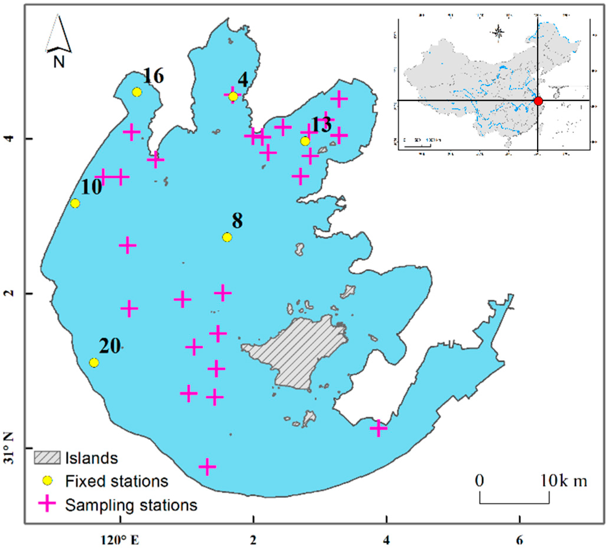
2.1. Study Area

With a drainage basin of 36,895 km², Taihu Lake is the third largest freshwater lake in China, having an average water depth of ~1.9 m and surface area of ~2338 km². The drainage basin covers some of the most developed regions in China including Jiangsu, Zhejiang, and Anhui Provinces and the Shanghai Municipality, which contributed ~10% of China’s GDP with only 0.4% of China’s territory [51,52]. In recent years, increasing eutrophication and cyanobacterial blooms have been reported, posing a significant threat the environment and humans who rely on the lake for drinking water, tourism, aquaculture, recreation, and other activities [9,53].

Several studies have shown locally optimized Chla algorithms for Taihu Lake [24,42,46], yet they are all based on in situ Rrs. Other studies used satellite data to show the multi-year cyanobacterial bloom patterns [8,9], but the index used in the studies is sensitive to only intense blooms when cyanobacteria form surface mats. To date, a practice Chla retrieval algorithm targeted for near real-time applications still needs to be developed.

2.2. Field Data

A series of cruise surveys were conducted by the Nanjing Institute of Geography and Limnology, Chinese Academy of Science (NIGLAS) between October 2004 and May 2011 (Figure 1). Six of these surveys measured surface Chla. Of these samples, after quality control and searching for the matching MODIS data records 28 were used in this study to develop the Chla retrieval algorithm. These surveys were conducted in October 2004, May 2008, October 2008, May 2010, March 2011, and May 2011.

In addition to the surveys, measurements were also collected at six fixed locations by NIGLAS (Figure 1). The data were collected weekly from April to September every year from 2008 to 2010. Total nitrogen, total phosphorus and Chla for the collected water samples were analyzed in the laboratory. Similar to the samples collected and measured during the field surveys, after data quality control and searching for the matching MODIS data 30 of these samples were used as the independent dataset used to validate the developed Chla algorithm.

Water samples were collected near the surface. Chla was then determined spectrophotometrically following community-accepted protocols [54,55]. Specifically, a 47-mm Whatman GF/F glass fiber filter was used to filter the water and was subsequently soaked in 90% ethanol for 4–6 h in the dark. The sample in ethanol was then heated to 80–90 °C for 3–5 min to extract the pigments. Absorbance at 665 and 750 nm of the extract was measured with a UV2401 spectrophotometer (Shimadzu Corp., Kyoto, Japan), and Chla was calculated against a blank reference (i.e., filtered water). There have been reports that Chla determined spectrophotometrically tended to be overestimated as compared with high-performance liquid chromatography (HPLC) method (e.g., Pinckney et al. [56]). However, the overestimation was small systematic bias instead of random error. Thus, the Chla dataset used in this study is self-consistent and will not impact algorithm development or studies on detecting anomalies.

Figure 1. Taihu Lake in the Yangtze River Delta, China. Annotated on the image are locations of the 28 sampling stations visited by the six NIGLAS cruise surveys (October 2004, May 2008, October 2008, May 2010, March 2011 and May 2011) and 6 fixed sampling sites.

Figure 1. Taihu Lake in the Yangtze River Delta, China. Annotated on the image are locations of the 28 sampling stations visited by the six NIGLAS cruise surveys (October 2004, May 2008, October 2008, May 2010, March 2011 and May 2011) and 6 fixed sampling sites.

2.3. MODIS Satellite Data

MODIS Level-0 data collected by both Terra (2000–present) and Aqua (2002–present) covering the study region were obtained from the NASA Goddard Space Flight Center through its Ocean Biology Processing Group [57]. With a swath width of 2330 km, the two MODIS instruments cover the Earth’s surface (including Taihu Lake) at least once per day, making this dataset suitable for near real-time applications. Both MODIS instruments have nine spectral bands from 412 to 869 nm at approximately 1-km ground resolution. These bands were designed for ocean use and are highly sensitive but with a narrow dynamic range [29]. They are saturated most of the time over Taihu Lake due to the turbid atmosphere and water, and therefore are not used in this study.

The MODIS instruments also have seven spectral bands from 469 nm to 2130 nm designed for land and atmosphere use. They are less sensitive but cover a higher dynamic range than the ocean bands, and therefore rarely saturate in this region. Although not designed for the ocean, the bands have shown wide applications for coastal and inland waters [8,58] because of their wide coverage and medium resolutions. The ground resolution of the 645- and 859-nm bands is 250 m, and 500 m for the bands at 469-, 555-, 1240-, 1640-, and 2130-nm. Because the 1240- and 1640-nm bands often contain substantial noise due to detector artifacts, in this study, only four bands at 469-, 555-, 645-, and 859-nm were used.

MODIS data were processed using the software SeaDAS (version 7.0). First, the data were converted to calibrated radiance (Level-1B). Then, because a full atmospheric correction through SeaDAS often resulted in data loss due to incorrect data masking and high uncertainties in the retrieved remote sensing reflectance (Rrs, sr⁻¹), a partial atmospheric correction to correct for the gaseous absorption (mainly by ozone) and Rayleigh (molecular) scattering effects was applied to the Level-1B data, resulting in Rayleigh corrected reflectance (Rrc, dimensionless):

R_rc(λ) =ρ_t(λ) − ρ_r(λ) = ρ_a(λ) + πt(λ)t₀(λ)Rrs(λ)

(1)

where ρ_t is the top of atmosphere (TOA) reflectance after adjustment of the gaseous absorption, ρ_r is the reflectance due to Rayleigh scattering, ρ_a is that due to aerosol scattering and aerosol-Rayleigh interactions, t and t₀ are diffuse transmittance from the image pixel to the satellite and from the sun to the image pixel, respectively. Note that ρ_a, t, and t₀ are functions of aerosol type, aerosol optical thickness, and solar/viewing geometry. The above formulation assumes negligible contributions from whitecaps and sun glint.

The Rrc data were mapped to a cylindrical equidistant projection for further analysis. First, the Rrc data at 645-nm, 555-nm, and 469-nm were used to compose the Red-Green-Blue true color images in order to screen for clouds and sun glint. After visual inspection, a total of 853 data granules between 2000 and 2013 were found to contain minimal cloud cover and sun glint, therefore suitable for algorithm development and time-series studies. The granules are evenly distributed in all four seasons, with approximately once per week frequency (Table 1). Potential aliasing due to infrequent measurements may be thus minimized at monthly to seasonal scales.

Table 1. Number of MODIS images used in each season, 2000–2013.

Season (Months)	# Of Images
Spring (April, May, June)	211
Summer (July, August, September)	192
Autumn (October, November, December)	203
Winter (January, February, March)	247
Total # of Images	853

Table 1. Number of MODIS images used in each season, 2000–2013.

Season (Months)	# Of Images
Spring (April, May, June)	211
Summer (July, August, September)	192
Autumn (October, November, December)	203
Winter (January, February, March)	247
Total # of Images	853

The Rrc data were then queried to find the data concurrent (same day) and collocated with the field measurements (termed “matching pairs”). For both algorithm development and validation, the following criteria were applied. To minimize the potential impact of straylight, a 3 × 3 pixel box centered at the field measurement location was selected. Only when at least five pixels of the 3 × 3 box contained valid Rrc data was the box used for further analysis. To assure spatial homogeneity, the variance of Rrc(555) in the box (standard deviation/mean) must be <10%, otherwise the box was discarded. The median value of the 3 × 3 box was used to compare with the field data. After quality control, only 28 field stations showed valid MODIS matching pairs (Figure 1), and these were used for algorithm development. Thirty other data points from the six fixed stations also showed MODIS matching pairs, and these were used to evaluate the algorithm.

To understand the impact of partial atmospheric correction (as compared with the full atmospheric correction) on the algorithm performance, a sensitivity test was conducted where various atmospheric parameters were extracted from the SeaDAS LUTs and passed to the algorithm as perturbations. These parameters include aerosol optical thickness at 869 nm (τ869), ρ_a, t₀, t, and extraterrestrial solar constant (F₀(λ)) corresponding to the solar/viewing geometry specified by the solar zenith angle (θo), satellite zenith angle (θ), and their relative azimuth angle (ϕ).

2.4. Algorithm Development

Figure 2a shows the MODIS Rrc spectra of the four land bands (469, 555, 645, 859 nm) corresponding to the 28 Chla matching pairs. Note that the high reflectance led to saturation of most of the MODIS 1-km ocean bands, leaving only four land bands to be used for the algorithm development.

Figure 2. (a) MODIS Rrc spectra (469, 555, 645, and 859 nm) corresponding to the 28 in situ measurements shown in Figure 1. These spectra were used with field-measured Chla to develop the EOF model; (b) MODIS Rrc ratios versus field-measured Chla.

Figure 2. (a) MODIS Rrc spectra (469, 555, 645, and 859 nm) corresponding to the 28 in situ measurements shown in Figure 1. These spectra were used with field-measured Chla to develop the EOF model; (b) MODIS Rrc ratios versus field-measured Chla.

Two existing algorithms were first tested to evaluate their performance. These are the blue-green band ratio algorithm following the traditional approach [59] and the red-green band ratio algorithm following the approach of [25]. The algorithms used the Rrc(469)/Rrc(555) and Rrc(645)/Rrc(555) ratios, respectively, to correlate with concurrent Chla. The Rrc(469)/Rrc(555) band ratio from MODIS had virtually no correlation with the field-measured Chla (Figure 2b). Although the Rrc(645)/Rrc(555) band ratio showed some correlation with the field-measured Chla, there was substantial data scattering. The poor performance of the band-ratio algorithms is mainly because that the band ratios were designed for Rrs instead of Rrc data, and the blue band contained information from not just particulate matter but also colored dissolved organic matter. Clearly, alternative approaches other than band ratios must be developed.

The EOF-based approach developed by [27] showed great potentials in deriving the water column IOPs, and it was adapted to estimate UV light attenuation in optically shallow waters in the Florida Keys from MODIS Rrs data in the visible bands [60] .The EOF approach is similar to principal component regression (PCR) or partial least squares (PLS) model, which have been used extensively in retrieving water quality parameters and land properties [61]. The EOF is used to reduce multi-band reflectance data to several independent (i.e., uncorrelated) variables (i.e., EOF modes or scores, aka eigenvectors) that retain most of the variance in the original data. Changes in the concentration of a water constituent (e.g., Chla) will affect the multi-band reflectance, thus will be correlated to one or more of the EOF modes. These modes can then be used in a stepwise fashion to reconstruct the corresponding Chla record, from which an empirical regression model is established. Further details of the original EOF approach and the modified approach can be found in [27,60], respectively. The approach was modified in this study to use the four-band MODIS Rrc data as the input. Specifically, the EOF analysis was implemented using the MATLAB™ function princomp. The input for this function consisted of an (N × m) array of Rrc(λ) spectra, where N was the number of samples, and m is the number of MODIS land band (m = 4). Following [27] and to focus on the variability in the spectral shape (as opposed to amplitude), MODIS Rrc spectra were normalized first:

$$\langle R_{rc}\left(\mathrm{\lambda }\right)\rangle =\frac{R_{rc}\left(\mathrm{\lambda }\right)}{{{\displaystyle \int }}_{469}^{859}{R}_{rc}\left(\mathrm{\lambda }\right)d\mathrm{\lambda }}$$

(2)

where <Rrc(λ)> is the normalized spectra [27,60]. EOFs were then constructed using the MODIS <Rrc(λ)>, with each EOF expressed as a vector of four loadings corresponding to the four spectral bands. Because only 4 MODIS bands were used in this analysis, the four EOF modes explained 100% of the variance in the <Rrc(λ)>. The resulting scores for each of these EOF modes were used as the independent variables in a stepwise multiple regression (i.e., stepwise principal component regression), with the dependent variable being the field-measured Chla.

2.5. Algorithm Evaluation

Several commonly accepted measures were used to assess algorithm performance. These include R² and Root-Mean-Square-Error (RMSE) in log space and unbiased RMSE (URMSE) in relative percentage (100%):

$$RMSE\left(log\right)=\sqrt{\frac{1}{N}{\displaystyle \sum }_{i=1}^N{\left(log10\left(y_i\right)-log10\left(x_i\right)\right)}^2}$$

(3)

$$URMSE\left(\text{\%}\right)=\sqrt{\frac{1}{N}{\displaystyle \sum }_{i=1}^N{(\frac{y_i-x_i}{0.5(y_i+x_i)})}^2}\times 100\text{\%}$$

(4)

where x_i and y_i refer to the measured and modeled values for the ith sample. The use of the log form was to follow the tradition for log-normal distributions [62]. URMSE (2(y − x)/(y + x)) was used instead of the typical RMSE ((y − x)/x) to avoid outliers that cause skewed error distributions [63]. This is particularly important when both x and y may contain large errors [64].

3. Results

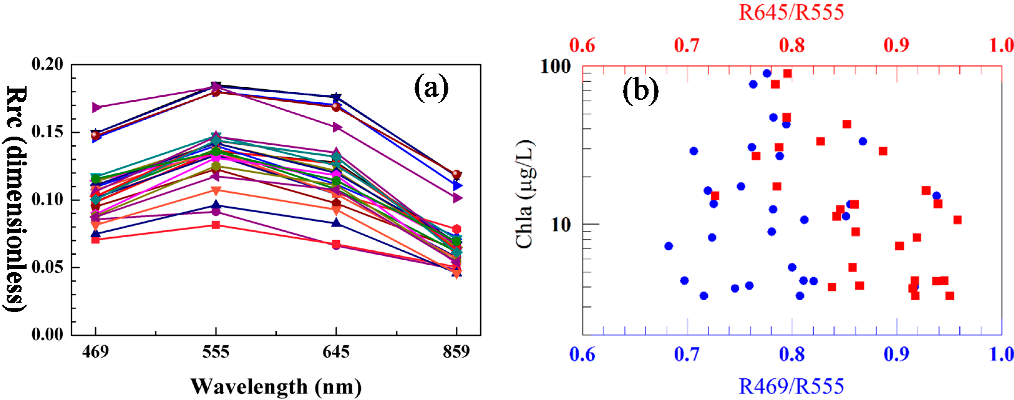
3.1. Algorithm Development

Figure 3a shows the algorithm performance using the 28 data pairs from MODIS and in situ measurements. Despite the data scattering around the 1:1 line, there is a statistically significant correlation between the EOF-modeled Chla and measured Chla, with coefficient of determination (R²) of 0.47. Unbiased RMSE is 63.3% and RMSE(log) is 0.29 for Chla ranging between ~3 and ~50 μg/L, slightly higher than that for the global open ocean (~0.27, [65]). Some of the data scatter might be caused by the possible patchiness in this optically complex lake and also potential errors in the measured Chla due to low sampling volume. Thus, the performance of the algorithm may be acceptable, especially when considering that only four land bands were used in the EOF-based algorithm and only a partial atmospheric correction was performed.

Figure 3. (a) Comparison between field measured Chla at the 28 stations (Figure 1) and Chla derived from the MODIS Rrc using the EOF model; (b) Validation of the EOF model using independent field measurements from the six fixed stations (Figure 1). The dashed lines are 1:1 lines.

Figure 3. (a) Comparison between field measured Chla at the 28 stations (Figure 1) and Chla derived from the MODIS Rrc using the EOF model; (b) Validation of the EOF model using independent field measurements from the six fixed stations (Figure 1). The dashed lines are 1:1 lines.

3.2. Algorithm Validation

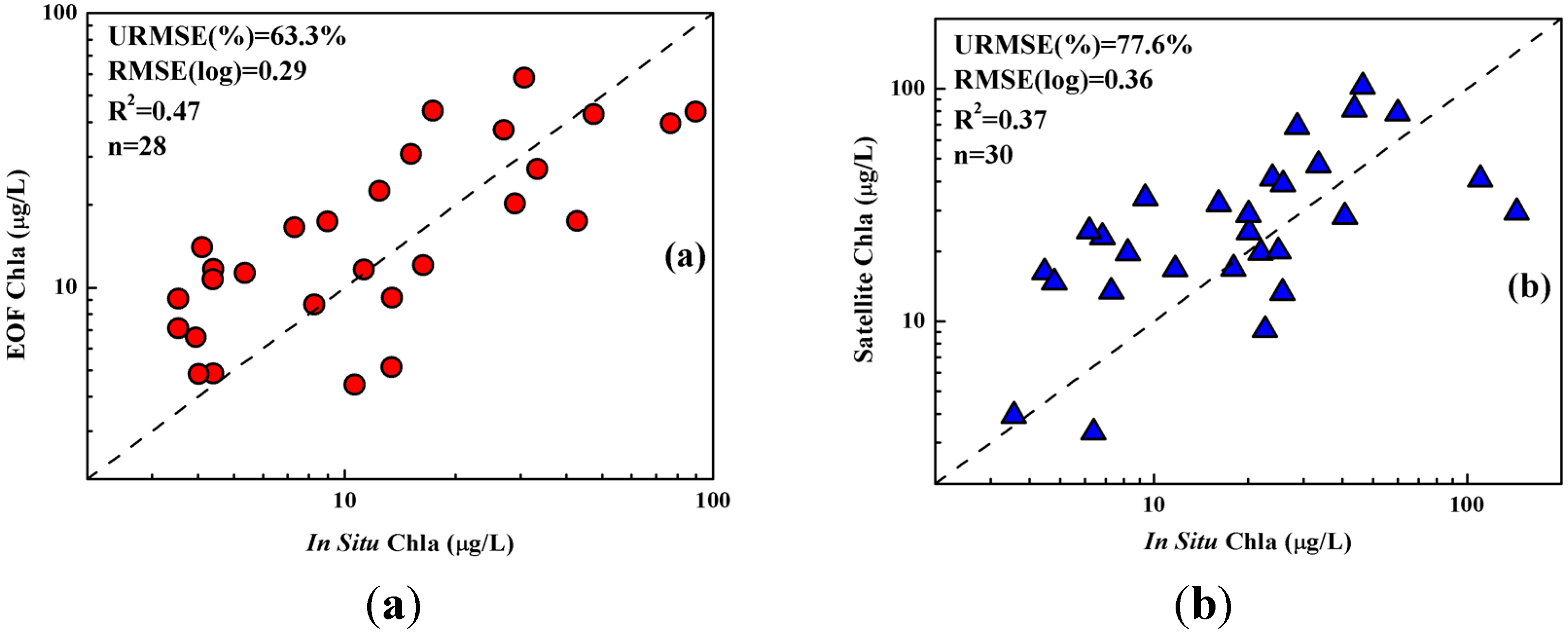
3.2.1. Validation Using MODIS Data and Field Data

The algorithm was further validated using independent data collected from the 6 fixed stations. The 30 matching pairs led to performance statistics slightly worse than those from the algorithm development (Figure 3b), with URMSE = 77.6%, RMSE(log) = 0.36, and R² = 0.37. However, for the same arguments as above, the performance might be acceptable as long as the retrieved Chla patterns are spatially coherent and temporally consistent, as shown below.

3.2.2. Validation Using MODIS Data Alone

Regardless of the amount of effort expended in collecting field data, these data are always limited in space and time. An additional method to validate algorithms is through consistency measures where satellite data products of adjacent days are examined for their spatial and temporal patterns. This method has been used in validating an open-ocean Chla algorithm developed recently for all ocean color sensors [64], and is adopted here.

First, the EOF-based algorithm was applied to all MODIS images. After a static landmask was applied, the images were screened to exclude pixels contaminated with clouds and sun glint [8]. Then, Rrc(λ) spectra from all valid pixels were normalized using Equation (4), which were then used as the input of the MATLAB™ princomp function to obtain the EOF scores for each Rrc spectrum (pixel). Finally, Chla for that pixel was derived as

$$\text{Chla}={\text{β}}_0+{\text{β}}_1{S}_1+{\text{β}}_2{S}_2+{\text{β}}_3{S}_3+{\text{β}}_4{S}_4$$

(5)

where β_0–4 are the regression coefficients derived from the 28 data pairs in the algorithm development, and S_1–4 are the EOF scores [27]. Note that of the four EOF scores only the first three would explain at least 5% of the variance from the input Rrc data, yet for completeness the fourth score is kept here. In contrast, for hyperspectral or multi-spectral data with many bands (e.g., 10 or more), for simplicity only the first several scores are used in the regression (e.g., [60]).

Such derived MODIS Chla images were examined one by one to determine whether Chla spatial patterns were coherent (i.e., there was no significant edging effect or sharp boundaries between different water masses) and whether Chla temporal patterns in the same locations were consistent under different observing conditions.

Figure 4. Performance of the Chla retrieval algorithm under different aerosol conditions in both winter (29 and 30 January 2007) and summer (8 and 9 August 2007). The top panels show MODIS RGB images (a,b,c,d) while the bottom panels show the retrieved Chla (e,f,g,h).The RGB images in winter (a,b) show significant variations in the aerosol content (haziness); yet the retrieved Chla images (e,f) are consistent in the large-scale spatial patterns and Chla magnitudes (e.g., higher Chla in the southern lake than in the northern lake); Likewise, for the bloom cases in summer, the retrieved Chla patterns in (g,h) appear to be insensitive to different aerosol perturbations in (c,d). Note that the optically shallow waters in the eastern lake are masked to prevent algorithm artifacts.

Figure 4. Performance of the Chla retrieval algorithm under different aerosol conditions in both winter (29 and 30 January 2007) and summer (8 and 9 August 2007). The top panels show MODIS RGB images (a,b,c,d) while the bottom panels show the retrieved Chla (e,f,g,h).The RGB images in winter (a,b) show significant variations in the aerosol content (haziness); yet the retrieved Chla images (e,f) are consistent in the large-scale spatial patterns and Chla magnitudes (e.g., higher Chla in the southern lake than in the northern lake); Likewise, for the bloom cases in summer, the retrieved Chla patterns in (g,h) appear to be insensitive to different aerosol perturbations in (c,d). Note that the optically shallow waters in the eastern lake are masked to prevent algorithm artifacts.

Figure 4 shows several examples of the algorithm performance under different aerosol perturbations for both non-bloom Figure 4a,b and bloom Figure 4c,d cases, respectively. For the non-bloom case in winter, the two MODIS images on consecutive days of 29 (Aqua) and 30 (Terra) January 2007 were collected under thin and thick aerosols, respectively, as revealed by the RGB images. The mean Rrc(859) differences between the two images was around 0.055, corresponding to aerosol optical thickness (τ_a) of 0.6 for maritime aerosols. Note that τ_a = 0.3 is the threshold for “thick aerosol” in the NASA processing software SeaDAS. Thus, even when the increased τ_a doubled the “thick aerosol” threshold (Figure 4a,b), the Chla spatial patterns were still temporally consistent for non-bloom conditions (Figure 4e,f). Likewise, for the two consecutive images on 8 August 2004 (Terra) and 9 August 2004 (Aqua) where mean Rrc(859) decreased by 0.036 (corresponding to τ_a decrease of 0.4, Figure 4c,d), most of the Chla spatial patterns for bloom conditions were also temporally consistent (Figure 4g,h). Note that the MODIS measurements were from both Terra (30 January 2007 and 8 August 2004) and Aqua (29 January 2007 and 9 August 2004), yet the EOF-retrieved Chla patterns are all consistent.

3.2.3. Sensitivity Test Using Radiative Transfer Simulations

Similar image comparison as shown in Figure 4 was performed for the entire MODIS time series, with similar findings, i.e., the EOF-based Chla algorithm appeared to be tolerant to aerosol perturbations. To further understand the algorithm sensitivity to aerosol perturbations under different solar/viewing geometry, radiative transfer simulations were used. In these simulations, aerosol perturbations (ρ_a(λ), t(λ), t₀(λ) in Equation (1)) to Rrc(λ) were estimated using SeaDAS aerosol look up tables (LUTs) for several scenarios. Specifically, variations in satellite zenith angle (scene edge or scene center), aerosol type (coastal or maritime), relative humidity and aerosol optical thickness were considered. Figure 5 shows that the EOF algorithm performance, in terms of URMSE and R², is roughly similar under these different circumstances, suggesting that the Rrc spectral shapes can be retrained under variable aerosol perturbations. This result is consistent to the image-based analysis (Figure 4).

Figure 5. Sensitivity of the EOF Chla algorithm to different aerosol perturbations, derived from radiative transfer simulations. (a) Coastal aerosol with relative humidity of 50%, τ_869 = 0.37 at the scene edge; (b) maritime aerosol with relative humidity of 90%, τ_869 = 0.51, scene edge; (c) coastal aerosol with relative humidity of 50%, τ_869 = 0.19, scene center; (d) maritime aerosol with relative humidity of 90%, τ_869 = 0.23, scene center.

Figure 5. Sensitivity of the EOF Chla algorithm to different aerosol perturbations, derived from radiative transfer simulations. (a) Coastal aerosol with relative humidity of 50%, τ_869 = 0.37 at the scene edge; (b) maritime aerosol with relative humidity of 90%, τ_869 = 0.51, scene edge; (c) coastal aerosol with relative humidity of 50%, τ_869 = 0.19, scene center; (d) maritime aerosol with relative humidity of 90%, τ_869 = 0.23, scene center.

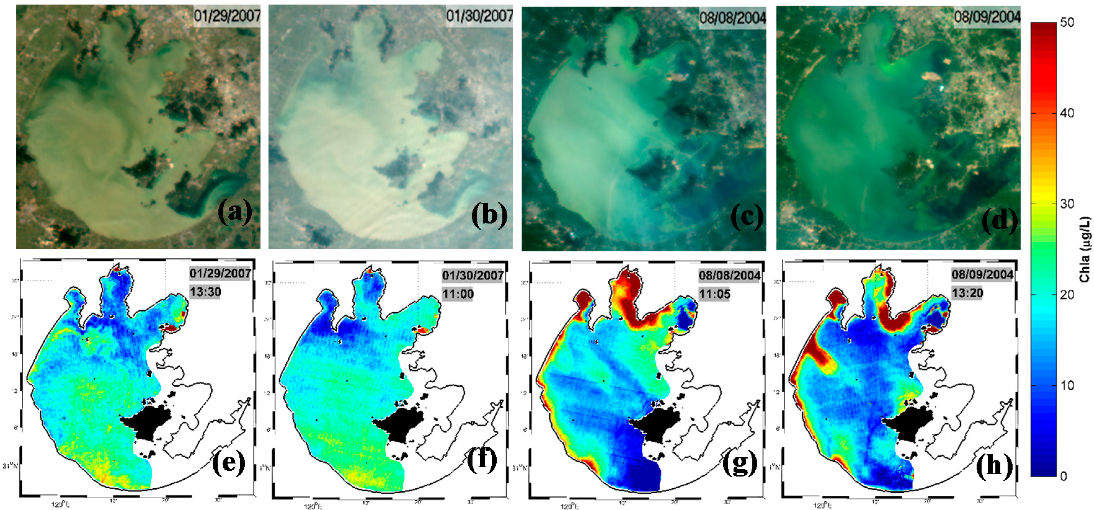
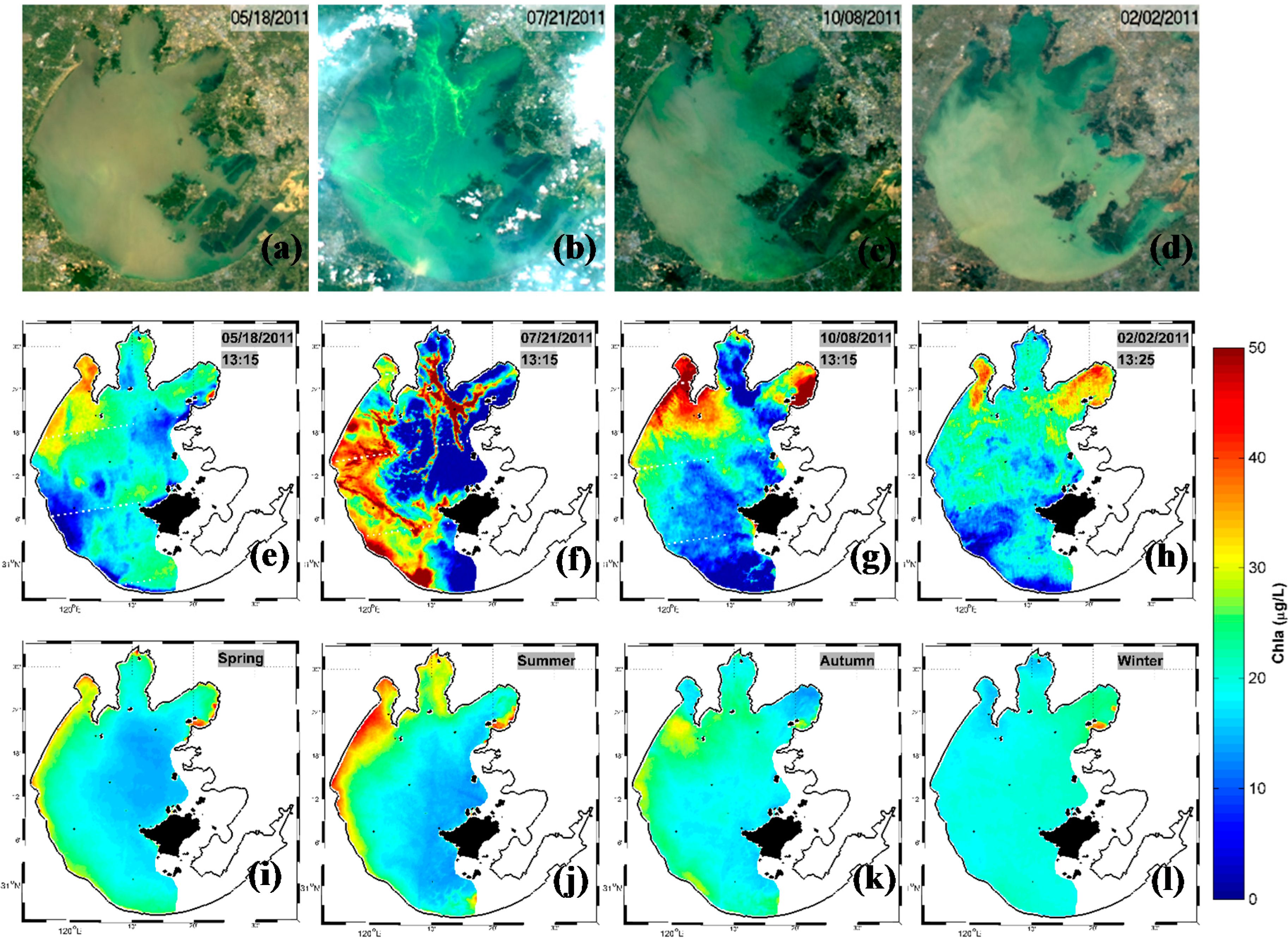
3.3. Application to Long-Term MODIS Data

Figure 6 shows the Chla spatial distributions in the four seasons derived by use of the EOF algorithm from MODIS Rrc data. The top panels in Figure 6a–d show the representative RGB images in the four seasons where bloom slicks and patches can be clearly visualized, and the middle panels show the corresponding Chla distributions. The summer image on 21 July 2011 reveals high Chla in the NW Lake, SW Lake, Meiliang Bay, Gonghu Bay, and north of the Central Lake due to typical cyanobacterial blooms in summer. The images in the other three seasons showed variable but generally lower Chla in the various lake segments, with generally higher Chla in the bays than in the Central Lake. The bottom panels in Figure 6 show the seasonal mean Chla distributions. Of the 853 MODIS images between 2000 and 2013, >200 images were used to calculate each seasonal mean. As such, the Chla patchiness in the individual images has been removed in the seasonal mean. Summer showed the highest Chla in the western lake and Meiliang Bay, followed by spring, fall, and winter. Such spatial distributions and their temporal changes are consistent with the findings of [8] where statistics of floating algae mats were used to estimate seasonal bloom variability. Unlike the algae mats assessment, the current study provides additional quantitative estimates of Chla distributions for assimilation in forecast models.

Figure 6. Examples of MODIS RGB and Chla in different seasons. The top panels (a–d) show MODIS RGB images selected in the four seasons, the middle panels (e–h) show the retrieved Chla corresponding to the RGB images, and the bottom panels (i–l) show the seasonal mean Chla between 2000 and 2013.

Figure 6. Examples of MODIS RGB and Chla in different seasons. The top panels (a–d) show MODIS RGB images selected in the four seasons, the middle panels (e–h) show the retrieved Chla corresponding to the RGB images, and the bottom panels (i–l) show the seasonal mean Chla between 2000 and 2013.

The MODIS Chla data were binned to calculate annual means and climatological monthly means for each of the six fixed sampling sites, with results shown in Figure 7. Despite the increasingly reported blooms in recent years, the 14-year trends in the annual means are not apparent in this dataset, although annual fluctuations are found in Figure 7a. In contrast, there is a clearly seasonality for most of the stations, with peak Chla between May and September (Figure 7b). Even though Chla in Taihu Lake could occasionally reach several hundreds of μg/L, such short-term variability has been smoothed in the annual and climatological monthly means, resulting in a relatively narrow range of Chla between 15 and 35 μg/L.

Figure 7. (a) Annual mean MODIS Chla and (b) Climatological monthly mean MODIS Chla for the six fixed sampling sites (Figure 1). Station 4 is in Meiliang Bay, Station 10 is in the NW Lake, and Station 8 is in the Central Lake.

Figure 7. (a) Annual mean MODIS Chla and (b) Climatological monthly mean MODIS Chla for the six fixed sampling sites (Figure 1). Station 4 is in Meiliang Bay, Station 10 is in the NW Lake, and Station 8 is in the Central Lake.

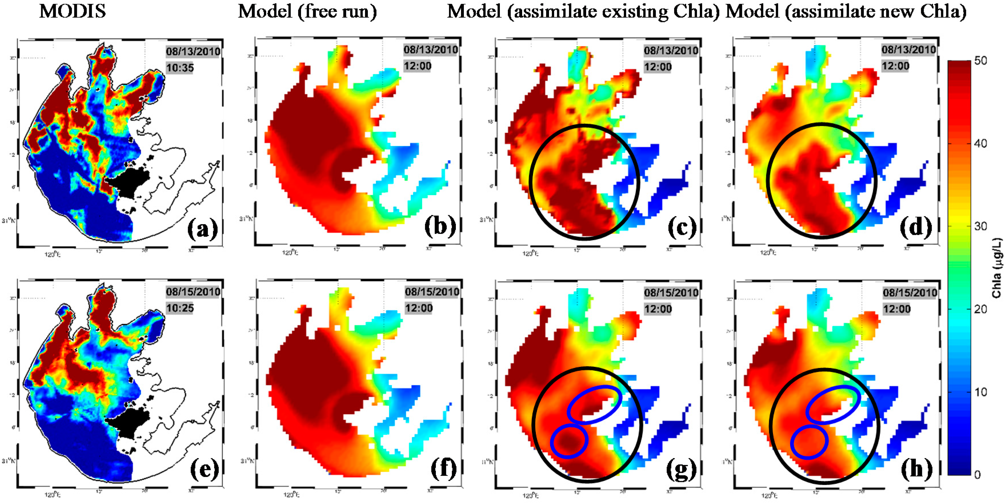
3.4. Data Assimilation Results Using Default Chla and New Chla: A Comparison

The EcoTaihu model [33] is a vertically-compressed three-dimensional ecological model. The model includes three modules: a relatively independent hydrodynamics module, a food chain network module, and a material transform and transport module. The model has been used to study water transfers from the Yangtze River to Taihu Lake [66] and to predict algal blooms [52]. The model parameterization, initialization, and forcing functions as well as other details can be found in [33], while the data assimilation method can be found in [43].

The model was initialized for 1 August 2010 and run through 31 August 2010, with a time step of 1 s and output every 24 h. The model initiation did not use any MODIS data, but used water quality data obtained from fixed monitoring stations during the previous month (July 2010) [33]. Three separate runs were conducted, with results shown in Figure 8. The first was a free run without assimilating MODIS data, used as the control (Figure 8b,f). The second run assimilated MODIS Chla distribution on 13 August 2010 derived from an existing back propagation (BP) algorithm that used only 2 MODIS bands at 645 and 859 nm [42] (Figure 8c,g). The third run assimilated MODIS Chla distribution on 13 August 2010 derived from the EOF algorithm in this study (Figure 8d,h).

Figure 8. Top panels in (a–d): Chla distributions on 13 August 2010. (a) MODIS (EOF algorithm); (b) Forecast model (EcoTaihu, started from 1 August) without assimilating MODIS data; (c) Forecast model after assimilating MODIS Chla from the existing BP algorithm [42]; (d) Forecast model after assimilating MODIS Chla from the new EOF algorithm (a). The forecast model (EcoTaihu) generated model output every 24 h on 12:00 AM local time. Bottom panels in (e–h): Chla distributions on 15 August 2010. Note that although the MODIS Chla image on 13 August was assimilated in the model, the MODIS Chla image on 15 August 2010 was not assimilated in the model and therefore served as a reference to validate the model’s performance in predicting Chla in two days.

Figure 8. Top panels in (a–d): Chla distributions on 13 August 2010. (a) MODIS (EOF algorithm); (b) Forecast model (EcoTaihu, started from 1 August) without assimilating MODIS data; (c) Forecast model after assimilating MODIS Chla from the existing BP algorithm [42]; (d) Forecast model after assimilating MODIS Chla from the new EOF algorithm (a). The forecast model (EcoTaihu) generated model output every 24 h on 12:00 AM local time. Bottom panels in (e–h): Chla distributions on 15 August 2010. Note that although the MODIS Chla image on 13 August was assimilated in the model, the MODIS Chla image on 15 August 2010 was not assimilated in the model and therefore served as a reference to validate the model’s performance in predicting Chla in two days.

Despite the model artifacts, there is some improvement in the model-predicted large-scale features. For example, the high-Chla patches outlined in the black circles appear to be unrealistic, and the use of the EOF-based MODIS Chla reduced such an artifact as compared with the use of the existing MODIS Chla (BP algorithm). This is especially apparent for the Chla patterns outlined in the blue circles. In general, there is a large difference between the model predicted Chla and MODIS-derived Chla (Figure 8e,h), suggesting future work is needed in model parameterization and tuning. Nevertheless, for the same model, the advantage of using the new EOF Chla over the old Chla in data assimilation is demonstrated here.

4. Discussion

Previous algorithm development for Taihu Lake and many other inland water bodies rarely used satellite data, but focused on field-measured Rrs (e.g., [24,67]). This may lead to two potential problems. One, the field data may not cover the full dynamic range of all environmental variables, limiting the application of the field-based algorithms to only those conditions under which the field data were collected. This is especially true when the field data were first classified before type-specific algorithms were developed. Two, the algorithms assumed error-free Rrs, which is not true for either field-measured or satellite-derived Rrs. Thus, in addition to the field-based algorithm development (which relies on both field and satellite measurements) and traditional point-based validation, this study also used image-based validation through inspection of the spatial and temporal patterns.

One aspect of this work is the use of Rrc instead of Rrs as a compromise between data quantity and data quality for near real-time use. Ideally, MODIS Rrs, after proper atmospheric correction, should be used for inversion to geophysical parameters such as Chla. However, although several case studies have shown significant improvement in turbid water atmospheric correction through using the MODIS shortwave infrared bands for Taihu Lake [68,69], the most significant problem for Taihu Lake real-time applications is lack of satellite data, as MODIS ocean bands often saturate over turbid atmosphere. Even without saturation, the requirements of the atmospheric correction on aerosol optical thickness (<0.3 at 869 nm) make valid MODIS Rrs retrievals extremely sparse for Taihu Lake. The MEdium Resolution Imaging Spectrometer (MERIS) has more spectral bands with more dynamic range, yet MERIS stopped functioning since April 2012. Several satellite missions are currently being planned by NASA and the European Space Agency (ESA). These include ESA’s Sentinel-III, which will have a MERIS-like sensor called Ocean and Land Color Instrument (OLCI, 300-m resolution) and is expected to launch around June 2015 (Bryan Franz, personal comm.). However, as with all previous ocean color missions, these future missions may also be delayed. The most recently launched Visible Infrared Imaging Radiometer Suite (VIIRS, 2012–present) may potentially be used for real-time applications, yet the calibration problems, especially after December 2012 (personal comm., Menghua Wang, NOAA NESDIS), make its performance unclear. Although not optimal, before VIIRS performance is evaluated, the use of MODIS Rrc from the land bands is perhaps the best available option. Yet future algorithm development efforts should be dedicated to VIIRS multi-spectral data once its calibration is improved, as VIIRS has more spectral bands than MODIS that do not saturate.

The limited number of MODIS bands, together with the large uncertainties in the full atmospheric correction, led to the EOF approach for near real-time Chla retrievals. Similar to other neural-network based approaches, the EOF is based the variance of the spectral reflectance and thus purely statistical without explaining the physical meaning of the EOF modes. However, the Chla spatial distribution patterns derived from the MODIS images appear reasonable. One reason may be due to the spectral normalization (Equation (4)), which may partially remove the aerosol effects while retaining most of the spectral shape information. Likewise, although the spectral magnitudes and shapes in the extracted MODIS Rrc data suggest sediment-rich waters, the influence of sediments on the Chla retrievals is implicitly suppressed by the EOF model tuning, as all the four spectral bands (especially the three visible bands) do contain information from phytoplankton. For example, the ratio of 645/555 reflectance has been shown highly correlated with Chla in Tampa Bay [70], and the 469-nm band is also influenced by phytoplankton pigment absorption. Nevertheless, given the large uncertainties and purely statistical nature of the algorithm, the EOF approach developed for the four MODIS bands is a temporary solution to derive large-scale Chla patterns in near real-time. This is especially true when considering that (1) Chla in the training dataset (about 3–100 μg/L) may not cover the full data range of all possible blooms, especially those during the summer. Zhang et al. (2009) showed Chla during all four seasons, and they reported median ± std of 31.6 ± 58.1 μg/L for summer, meaning that about 25% of their data are above 100 μg/L (i.e., exceeding the data range used in this study)[49]. Although some of the MODIS images showed that the algorithm could retrieve Chla > 100 μg/L (especially over surface scums), the validity of these high-Chla values needs to be verified; (2) perturbations from sun glint, thin clouds, whitecaps, and other aerosol types that were not used in the sensitivity simulations (Figure 5) could induce additional uncertainties in the algorithm. Figure 5 shows that compared with the original URMSE of 63.3% in the Rrs-based algorithm development (Figure 3a), most aerosol perturbations could induce another 5% in the URMSE. Other perturbations that were not considered in the simulations could possibly induce extra 5% or 10% URMSE, leading to a total URMS approaching or even higher than 80%. Clearly, future efforts should be dedicated to collect more field-MODIS data pairs to fine tune and improve the algorithm under most, if not all, satellite measurement conditions.

The limited model runs results also suggest the need for improvement of forecasting models. Over the last two decades, two general approaches have been developed to forecast Chla. The first was based on statistics through either regression [71], artificial neural networks [72,73], or fuzzy logic [74]. The second was based on physical and biological processes, which could reveal controlling factors and causal relationships [75,76,77,78,79,80]. For Taihu Lake, such process-oriented models have been developed and used to study hydrodynamics and biological response to physical forcing [33,52,81,82]. However, application of such a model together with MODIS data assimilation revealed large-scale artifacts, where the reasons need to be further diagnosed. For example, it might be possible that the model has inherent limitations due to the shallow water bottom (mean water depth of Taihu Lake is ~2 m), which presents a dragging force but is neglected in nearly all hydrodynamic models. Nevertheless, even with such apparent model artifacts, the improvement in MODIS Chla still led to improved performance in the model prediction. Clearly, an inter-disciplinary effort is required to improve both the forecast model and the MODIS Chla retrievals in order to implement a near real-time operational forecasting model for Taihu Lake.

Can the EOF approach be applied to other similar water bodies in different geographical and biogeochemical regimes where MODIS ocean bands also saturate? A preliminary test of the algorithm using data collected from a nearby lake, Chaohu Lake, showed reasonable Chla distribution patterns although their validity still requires rigorous validation. It is believed that similar to previous EOF approaches to retrieve water quality parameters [27,60], the principle of the EOF approach should be applicable to other similar water bodies for most water quality parameters including Chla, yet the number of spectral bands, number of modes, and parameterization of the algorithm may need to be localized to account for the different bio-optical properties (e.g., dominated by suspended sediments, CDOM, or phytoplankton). We anticipate carrying out these experiments for other lakes in the near future.

5. Conclusions

This work represents one step towards the ultimate goal of establishing an operational, near real-time forecast model to predict Chla distribution in a turbid lake. Using in situ data and only four MODIS land bands that do not saturate over turbid atmosphere or turbid water, the empirical approach based on Empirical Orthogonal Function (EOF) analysis provides a preliminary solution to derive Chla under cloudfree conditions in near real-time for Taihu Lake of China, which can be assimilated in forecast models to improve Chla prediction. For Chla ranging between 3 and 100 μg/L, the unbiased RMS uncertainties were estimated to be <80%. Together with 853 cloud-free MODIS images between 2000 and 2013, the algorithm led to the development of spatial and temporal Chla distribution patterns in Taihu Lake. The preliminary success is encouraging as MODIS is currently the only well calibrated operational sensor for near real-time applications, yet the large uncertainties and the limited number of spectral bands suggest further improvements in both the Chla retrieval algorithms and data availability from future satellite sensors. The discrepancy between model predictions and satellite observations also points to the need of improving the forecasting models.

References

- Kahru, M.; Mitchell, B.G. Ocean color reveals increased blooms in various parts of the world. Eos Trans. Am. Geophys. Union 2008. [Google Scholar] [CrossRef]
- Lapointe, B.E.; Langton, R.; Bedford, B.J.; Potts, A.C.; Day, O.; Hu, C. Land-based nutrient enrichment of the Buccoo Reef Complex and fringing coral reefs of Tobago, West Indies. Mar. Pollut. Bull. 2010, 60, 334–343. [Google Scholar] [CrossRef] [PubMed]
- Beman, J.M.; Arrigo, K.R.; Matson, P.A. Agricultural runoff fuels large phytoplankton blooms in vulnerable areas of the ocean. Nature 2005, 434, 211–214. [Google Scholar] [CrossRef] [PubMed]
- Brand, L.E.; Compton, A. Long-term increase in Karenia brevis abundance along the Southwest Florida Coast. Harmful Algae 2007, 6, 232–252. [Google Scholar] [CrossRef] [PubMed]
- Zhou, M.; Zhou, M. Progress of the project ecology and oceanography of harmful algal blooms in China. Adv. Earth Sci. 2006, 21, 673–679. (In Chinese) [Google Scholar]
- Liu, D.; Keesing, J.K.; Xing, Q.; Shi, P. World’s largest macroalgal bloom caused by expansion of seaweed aquaculture in China. Mar. Pollut. Bull. 2009, 58, 888–895. [Google Scholar] [CrossRef] [PubMed]
- Hu, C.; Li, D.; Chen, C.; Ge, J.; Muller-Karger, F.E.; Liu, J.; Yu, F.; He, M.X. On the recurrent Ulva prolifera blooms in the Yellow Sea and East China Sea. J. Geophys. Res.: Oceans (1978–2012) 2010, 115. [Google Scholar] [CrossRef]
- Hu, C.; Lee, Z.; Ma, R.; Yu, K.; Li, D.; Shang, S. Moderate resolution imaging spectroradiometer (MODIS) observations of cyanobacteria blooms in Taihu Lake, China. J. Geophys. Res. Oceans (1978–2012) 2010, 115. [Google Scholar] [CrossRef]
- Duan, H.; Ma, R.; Xu, X.; Kong, F.; Zhang, S.; Kong, W.; Hao, J.; Shang, L. Two-decade reconstruction of algal blooms in China’s Lake Taihu. Environ. Sci. Technol. 2009, 43, 3522–3528. [Google Scholar] [CrossRef] [PubMed]
- Schaeffer, B.A.; Hagy, J.D.; Conmy, R.N.; Lehrter, J.C.; Stumpf, R.P. An approach to developing numeric water quality criteria for coastal waters using the SeaWiFS satellite data record. Environ. Sci. Technol. 2012, 46, 916–922. [Google Scholar] [CrossRef] [PubMed]
- Anderson, D.M. Approaches to monitoring, control and management of harmful algal blooms (HABs). Ocean Coast. Manag. 2009, 52, 342–347. [Google Scholar] [CrossRef] [PubMed]
- Kudela, R.; Seeyave, S.; Cochlan, W. The role of nutrients in regulation and promotion of harmful algal blooms in upwelling systems. Prog. Oceanogr. 2010, 85, 122–135. [Google Scholar] [CrossRef]
- Bouma, J.; Van der Woerd, H.; Kuik, O. Assessing the value of information for water quality management in the North Sea. J. Environ. Manag. 2009, 90, 1280–1288. [Google Scholar] [CrossRef]
- Kong, F.; Ma, R.; Gao, J.; Wu, X. The theory and practice of prevention, forecast and warning on cyanobacteria bloom in Lake Taihu. J. Lake Sci. 2009, 3, 314–328. [Google Scholar]
- Sellner, K.G.; Doucette, G.J.; Kirkpatrick, G.J. Harmful algal blooms: Causes, impacts and detection. J. Ind. Microbiol. Biotechnol. 2003, 30, 383–406. [Google Scholar] [CrossRef] [PubMed]
- Pierson, D.C.; Strömbeck, N. A modelling approach to evaluate preliminary remote sensing algorithms: Use of water quality data from Swedish Great Lakes. Geophysica 2000, 36, 177–202. [Google Scholar]
- Thiemann, S.; Kaufmann, H. Determination of chlorophyll content and trophic state of lakes using field spectrometer and IRS-1C satellite data in the Mecklenburg Lake District, Germany. Remote Sens. Environ. 2000, 73, 227–235. [Google Scholar] [CrossRef]
- Ruddick, K.G.; Gons, H.J.; Rijkeboer, M.; Tilstone, G. Optical remote sensing of chlorophyll a in case 2 waters by use of an adaptive two-band algorithm with optimal error properties. Appl. Opt. 2001, 40, 3575–3585. [Google Scholar] [CrossRef]
- Tassan, S.; Ferrari, G.M. Variability of light absorption by aquatic particles in the near-infrared spectral region. Appl. Opt. 2003, 42, 4802–4810. [Google Scholar] [CrossRef]
- Dal’Olmo, G.; Gitelson, A.A.; Rundquist, D.C.; Leavitt, B.; Barrow, T.; Holz, J.C. Assessing the potential of SeaWiFS and MODIS for estimating chlorophyll concentration in turbid productive waters using red and near-infrared bands. Remote Sens. Environ. 2005, 96, 176–187. [Google Scholar] [CrossRef]
- Jiao, H.; Zha, Y.; Gao, J.; Li, Y.; Wei, Y.; Huang, J. Estimation of chlorophyll a concentration in Lake Tai, China using in situ hyperspectral data. Int. J. Remote Sens. 2006, 27, 4267–4276. [Google Scholar] [CrossRef]
- Tzortziou, M.; Herman, J.R.; Gallegos, C.L.; Neale, P.J.; Subramaniam, A.; Harding, L.W., Jr.; Ahmad, Z. Bio-optics of the Chesapeake Bay from measurements and radiative transfer closure. Estuar. Coast. Shelf Sci. 2006, 68, 348–362. [Google Scholar] [CrossRef]
- Gitelson, A.A.; Dall’Olmo, G.; Moses, W.; Rundquist, D.C.; Barrow, T.; Fisher, T.R.; Gurlin, D.; Holz, J. A simple semi-analytical model for remote estimation of chlorophyll-a in turbid waters: Validation. Remote Sens. Environ. 2008, 112, 3582–3593. [Google Scholar]
- Le, C.; Li, Y.; Zha, Y.; Sun, D.; Huang, C.; Lu, H. A four-band semi-analytical model for estimating chlorophyll a in highly turbid lakes: The case of Taihu Lake, China. Remote Sens. Environ. 2009, 113, 1175–1182. [Google Scholar] [CrossRef]
- Le, C.; Hu, C.; English, D.; Cannizzaro, J.; Kovach, C. Climate-driven chlorophyll-a changes in a turbid estuary: Observations from satellites and implications for management. Remote Sens. Environ. 2013, 130, 11–24. [Google Scholar] [CrossRef]
- Keiner, L. Estimating oceanic chlorophyll concentrations with neural networks. Int. J. Remote Sens. 1999, 20, 189–194. [Google Scholar]
- Craig, S.E.; Jones, C.T.; Li, W.K.; Lazin, G.; Horne, E.; Caverhill, C.; Cullen, J.J. Deriving optical metrics of coastal phytoplankton biomass from ocean colour. Remote Sens. Environ. 2012, 119, 72–83. [Google Scholar] [CrossRef]
- Hu, C.; Barnes, B.B.; Murch, B.; Carlson, P. Satellite-based virtual buoy system to monitor coastal water quality. Opt. Eng. 2014, 53, 051402–051402. [Google Scholar] [CrossRef]
- Hu, C.; Feng, L.; Lee, Z.; Davis, C.O.; Mannino, A.; McClain, C.R.; Franz, B.A. Dynamic range and sensitivity requirements of satellite ocean color sensors: Learning from the past. Appl. Opt. 2012, 51, 6045–6062. [Google Scholar] [CrossRef] [PubMed]
- Le, C.; Hu, C.; Cannizzaro, J.; Duan, H. Long-term distribution patterns of remotely sensed water quality parameters in Chesapeake Bay. Estuar. Coast. Shelf Sci. 2013, 128, 93–103. [Google Scholar] [CrossRef]
- Millie, D.F.; Weckman, G.R.; Young, W.A., II; Ivey, J.E.; Fries, D.P.; Ardjmand, E.; Fahnenstiel, G.L. Coastal “Big Data” and nature-inspired computation: Prediction potentials, uncertainties, and knowledge derivation of neural networks for an algal metric. Estuar. Coast. Shelf Sci. 2013, 125, 57–67. [Google Scholar]
- Popova, E.; Lozano, C.; Srokosz, M.; Fasham, M.; Haley, P.; Robinson, A. Coupled 3D physical and biological modelling of the mesoscale variability observed in North-East Atlantic in spring 1997: Biological processes. Deep Sea Res. Part I: Oceanogr. Res. Pap. 2002, 49, 1741–1768. [Google Scholar] [CrossRef]
- Hu, W.; Jørgensen, S.E.; Zhang, F. A vertical-compressed three-dimensional ecological model in Lake Taihu, China. Ecol. Model. 2006, 190, 367–398. [Google Scholar] [CrossRef]
- Anderson, L.A.; Robinson, A.R.; Lozano, C.J. Physical and biological modeling in the Gulf Stream region: I Data assimilation methodology. Deep Sea Res. Part I: Oceanogr. Res. Pap. 2000, 47, 1787–1827. [Google Scholar] [CrossRef]
- Natvik, L.-J.; Evensen, G. Assimilation of ocean colour data into a biochemical model of the North Atlantic: Part 1. Data assimilation experiments. J. Mar. Syst. 2003, 40, 127–153. [Google Scholar] [CrossRef]
- Nerger, L.; Gregg, W.W. Assimilation of SeaWiFS data into a global ocean-biogeochemical model using a local SEIK filter. J. Mar. Syst. 2007, 68, 237–254. [Google Scholar] [CrossRef] [Green Version]
- Tjiputra, J.F.; Polzin, D.; Winguth, A.M. Assimilation of seasonal chlorophyll and nutrient data into an adjoint three-dimensional ocean carbon cycle model: Sensitivity analysis and ecosystem parameter optimization. Glob. Biogeochem. Cycles 2007, 21. [Google Scholar] [CrossRef]
- Mao, J.; Lee, J.H.; Choi, K. The extended Kalman filter for forecast of algal bloom dynamics. Water Res. 2009, 43, 4214–4224. [Google Scholar] [CrossRef] [PubMed]
- Hu, J.; Fennel, K.; Mattern, J.P.; Wilkin, J. Data assimilation with a local Ensemble Kalman Filter applied to a three-dimensional biological model of the Middle Atlantic Bight. J. Mar. Syst. 2012, 94, 145–156. [Google Scholar] [CrossRef]
- Huang, J.; Gao, J.; Liu, J.; Zhang, Y. State and parameter update of a hydrodynamic-phytoplankton model using ensemble Kalman filter. Ecol. Model. 2013, 263, 81–91. [Google Scholar] [CrossRef]
- Ishizaka, J. Coupling of coastal zone color scanner data to a physical-biological model of the southeastern US continental shelf ecosystem: 2. An Eulerian model. J. Geophys. Res.: Oceans (1978–2012) 1990, 95, 20183–20199. [Google Scholar] [CrossRef]
- Qi, L.; Ma, R.; Hu, W.; Loiselle, S.A. Assimilation of MODIS chlorophyll a data into a coupled hydrodynamic-biological model of Taihu Lake. IEEE J. Sel. Top. Appl. Earth Obs. Remote Sens. 2014, 7, 1623–1631. [Google Scholar]
- Kong, W.; Ma, R.; Duan, H. The neural network model for estimation of chlorophyll-a with water temperature in Lake Taihu. J. Lake Sci. 2009, 21, 193–198. [Google Scholar]
- Gons, H.J. Optical teledetection of chlorophyll a in turbid inland waters. Environ. Sci. Technol. 1999, 33, 1127–1132. [Google Scholar] [CrossRef]
- Han, L.; Rundquist, D.C. Comparison of NIR/RED ratio and first derivative of reflectance in estimating algal-chlorophyll concentration: A case study in a turbid reservoir. Remote Sens. Environ. 1997, 62, 253–261. [Google Scholar] [CrossRef]
- Ma, R.; Dai, J. Investigation of chlorophyll a and total suspended matter concentrations using Landsat ETM and field spectral measurement in Taihu Lake, China. Int. J. Remote Sens. 2005, 26, 2779–2795. [Google Scholar] [CrossRef]
- Yacobi, Y.Z.; Moses, W.J.; Kaganovsky, S.; Sulimani, B.; Leavitt, B.C.; Gitelson, A.A. NIR-red reflectance-based algorithms for chlorophyll-a estimation in mesotrophic inland and coastal waters: Lake Kinneret case study. Water Res. 2011, 45, 2428–2436. [Google Scholar] [CrossRef] [PubMed]
- Zhang, Y.; Liu, M.; Qin, B.; Van der Woerd, H.J.; Li, J.; Li, Y. Modeling remote-sensing reflectance and retrieving chlorophyll-a concentration in extremely turbid Case-2 waters (Lake Taihu, China). IEEE Trans. Geosci. Remote Sens. 2009, 47, 1937–1948. [Google Scholar] [CrossRef]
- Kahru, M.; Kudela, R.M.; Anderson, C.R.; Manzano-Sarabia, M.; Mitchell, B.G. Evaluation of satellite retrievals of ocean chlorophyll-a in the California Current. Remote Sens. 2014, 6, 8524–8540. [Google Scholar] [CrossRef]
- Blondeau-Patissier, D.; Gower, J.F.R.; Dekker, A.G.; Phinn, S.R.; Brando, V.E. A review of ocean color remote sensing methods and statistical techniques for the detection, mapping and analysis of phytoplankton blooms in coastal and open oceans. Prog. Oceanogr. 2014, 123, 123–144. [Google Scholar] [CrossRef] [Green Version]
- Qin, B.; Xu, P.; Wu, Q.; Luo, L.; Zhang, Y. Environmental issues of lake Taihu, China. Hydrobiologia 2007, 581, 3–14. [Google Scholar] [CrossRef]
- Zhang, H.; Hu, W.; Gu, K.; Li, Q.; Zheng, D.; Zhai, S. An improved ecological model and software for short-term algal bloom forecasting. Environ. Model. Softw. 2013, 48, 152–162. [Google Scholar] [CrossRef]
- Guo, L. Doing battle with the green monster of Taihu Lake. Science 2007, 317, 1166–1166. [Google Scholar] [CrossRef] [PubMed]
- Ma, R.; Tang, J.; Dai, J.; Zhang, Y.; Song, Q. Absorption and scattering properties of water body in Taihu Lake, China: Absorption. Int. J. Remote Sens. 2006, 27, 4277–4304. [Google Scholar] [CrossRef]
- Ma, R.; Tang, J.; Dai, J. Bio-optical model with optimal parameter suitable for Taihu Lake in water colour remote sensing. Int. J. Remote Sens. 2006, 27, 4305–4328. [Google Scholar]
- Pinckney, J.; Papa, R.; Zingmark, R. Comparison of high-performance liquid chromatographic, spectrophotometric, and fluorometric methods for determining chlorophyll a concentrations in estaurine sediments. J. Microbiol. Methods 1994, 19, 59–66. [Google Scholar] [CrossRef]
- NASA Ocean Biology Processing Group. OceanColor Web. Available online: http://oceancolor.gsfc.nasa.gov (accessed on 15 February 2014).
- Hu, C.; Chen, Z.; Clayton, T.D.; Swarzenski, P.; Brock, J.C.; Muller-Karger, F.E. Assessment of estuarine water-quality indicators using MODIS medium-resolution bands: Initial results from Tampa Bay, FL. Remote Sens. Environ. 2004, 93, 423–441. [Google Scholar] [CrossRef]
- O’Reilly, J.; Maritorena, S.; Siegel, D.; Siegel, D.A.; Margaret, C.; Dierdre, T.; Greg, M.; Mati, K.; Francisco, P.C.; Strutton, P.; et al. Ocean color chlorophyll a algorithms for SeaWiFS, OC2, and OC4: Version 4. In SeaWiFS Postlaunch Technical Report Series, Volume 11, SeaWiFS Postlaunch Calibration and Validation Analyses, Part 3; Hooker, S.B., Firestone, E.R., Eds.; NASA, Goddard Space Flight Center: Greenbelt, MD, USA, 2000; pp. 8–23. [Google Scholar]
- Barnes, B.B.; Hu, C.; Cannizzaro, J.P.; Craig, S.E.; Hallock, P.; Jones, D.L.; Lehrter, J.C.; Melo, N.; Schaeffer, B.A.; Zepp, R.; et al. Estimation of diffuse attenuation of ultraviolet light in optically shallow Florida Keys waters from MODIS measurements. Remote Sens. Environ. 2014, 140, 519–532. [Google Scholar] [CrossRef]
- Song, K.; Li, L.; Tedesco, L.P.; Li, S.; Clercin, N.A.; Hall, B.E.; Li, Z.; Shi, K. Hyperspectral determination of eutrophication for a water supply source via genetic algorithm-partial least squares (GA-PLS) modeling. Sci. Total Environ. 2012, 426, 220–232. [Google Scholar] [PubMed]
- Campbell, J.W. The lognormal distribution as a model for bio-optical variability in the sea. J. Geophys. Res.: Oceans (1978–2012) 1995, 100, 13237–13254. [Google Scholar] [CrossRef]
- Hooker, S.B.; Lazin, G.; Zibordi, G.; McLean, S. An evaluation of above- and in-water methods for determining water-leaving radiances. J. Atmos. Ocean. Technol. 2002, 19, 486–515. [Google Scholar] [CrossRef]
- Hu, C.; Lee, Z.; Franz, B. Chlorophyll a algorithms for oligotrophic oceans: A novel approach based on three-band reflectance difference. J. Geophys. Res.: Oceans (1978–2012) 2012, 117. [Google Scholar] [CrossRef]
- Gregg, W.W.; Casey, N.W. Global and regional evaluation of the SeaWiFS chlorophyll data set. Remote Sens. Environ. 2004, 93, 463–479. [Google Scholar]
- Hu, W.; Zhai, S.; Zhu, Z.; Han, H. Impacts of the Yangtze River water transfer on the restoration of Lake Taihu. Ecol. Eng. 2008, 34, 30–49. [Google Scholar]
- Duan, H.; Ma, R.; Zhang, Y.; Loiselle, S.A.; Xu, J.; Zhao, C.; Zhou, L.; Shang, L. A new three-band algorithm for estimating chlorophyll concentrations in turbid inland lakes. Environ. Res. Lett. 2010, 5. [Google Scholar] [CrossRef]
- Wang, M.; Shi, W.; Tang, J. Water property monitoring and assessment for China’s inland Lake Taihu from MODIS-Aqua measurements. Remote Sens. Environ. 2011, 115, 841–854. [Google Scholar] [CrossRef]
- Zhang, M.; Ma, R.; Li, J.; Zhang, B.; Duan, H. A validation study of an improved SWIR iterative atmospheric correction algorithm for MODIS-Aqua measurements in Lake Taihu, China. IEEE Trans. Geosci. Remote Sens. 2014, 52, 4686–4695. [Google Scholar] [CrossRef]
- Le, C.; Hu, C.; English, D.; Cannizzaro, J.; Chen, Z.; Feng, L.; Boler, R.; Kovach, C. Towards a long-term chlorophyll a data record in a turbid estuary using MODIS observations. Prog. Oceanogr. 2013, 109, 90–103. [Google Scholar] [CrossRef]
- Chen, Y.; Qin, B.; Gao, X. Prediction of blue-green algae bloom using stepwise multiple regression between algae & related environmental factors in Meiliang Bay, Lake Taihu. J. Lake Sci. 2001, 1, 63–71. [Google Scholar]
- Lee, J.H.; Huang, Y.; Dickman, M.; Jayawardena, A. Neural network modelling of coastal algal blooms. Ecol. Model. 2003, 159, 179–201. [Google Scholar] [CrossRef]
- Muttil, N.; Chau, K.-W. Neural network and genetic programming for modelling coastal algal blooms. Int. J. Environ. Pollut. 2006, 28, 223–238. [Google Scholar]
- Laanemets, J.; Lilover, M.-J.; Raudsepp, U.; Autio, R.; Vahtera, E.; Lips, I.; Lips, U. A fuzzy logic model to describe the cyanobacteria Nodularia spumigena blooms in the Gulf of Finland, Baltic Sea. Hydrobiologia 2006, 554, 31–45. [Google Scholar] [CrossRef]
- Hamilton, D.P.; Schladow, S.G. Prediction of water quality in lakes and reservoirs Part I—Model description. Ecol. Model. 1997, 96, 91–110. [Google Scholar] [CrossRef]
- Schladow, S.G.; Hamilton, D.P. Prediction of water quality in lakes and reservoirs: Part II—Model calibration, sensitivity analysis and application. Ecol. Model. 1997, 96, 111–123. [Google Scholar] [CrossRef]
- Sacau-Cuadrado, M.; Conde-Pardo, P.; Otero-Tranchero, P. Forecast of red tides off the Galician coast. Acta Astronaut. 2003, 53, 439–443. [Google Scholar] [CrossRef]
- Allen, J.; Smyth, T.J.; Siddorn, J.R.; Holt, M. How well can we forecast high biomass algal bloom events in a eutrophic coastal sea? Harmful Algae 2008, 8, 70–76. [Google Scholar] [CrossRef]
- Los, F.; Villars, M.; Van der Tol, M. A 3-dimensional primary production model (BLOOM/GEM) and its applications to the (southern) North Sea (coupled physical-chemical-ecological model). J. Mar. Syst. 2008, 74, 259–294. [Google Scholar] [CrossRef]
- Jørgensen, S.E.; Bendoricchio, G. Fundamentals of Ecological Modelling; Elsevier: Oxford, UK, 2001. [Google Scholar]
- Li, W.; Qin, B.; Zhu, G. Forecasting short-term cyanobacterial blooms in Lake Taihu, China, using a coupled hydrodynamic-algal biomass model. Ecohydrology 2013, 7, 794–802. [Google Scholar]
- Huang, J.; Gao, J.; Hörmann, G. Hydrodynamic-phytoplankton model for short-term forecasts of phytoplankton in Lake Taihu, China. Limnol. Ecol. Manag. Inland Waters 2012, 42, 7–18. [Google Scholar] [CrossRef]
© 2014 by the authors; licensee MDPI, Basel, Switzerland. This article is an open access article distributed under the terms and conditions of the Creative Commons Attribution license (http://creativecommons.org/licenses/by/4.0/).
Share and Cite
Qi, L.; Hu, C.; Duan, H.; Barnes, B.B.; Ma, R. An EOF-Based Algorithm to Estimate Chlorophyll a Concentrations in Taihu Lake from MODIS Land-Band Measurements: Implications for Near Real-Time Applications and Forecasting Models. Remote Sens. 2014, 6, 10694-10715. https://doi.org/10.3390/rs61110694
Qi L, Hu C, Duan H, Barnes BB, Ma R. An EOF-Based Algorithm to Estimate Chlorophyll a Concentrations in Taihu Lake from MODIS Land-Band Measurements: Implications for Near Real-Time Applications and Forecasting Models. Remote Sensing. 2014; 6(11):10694-10715. https://doi.org/10.3390/rs61110694
Chicago/Turabian StyleQi, Lin, Chuanmin Hu, Hongtao Duan, Brian B. Barnes, and Ronghua Ma. 2014. "An EOF-Based Algorithm to Estimate Chlorophyll a Concentrations in Taihu Lake from MODIS Land-Band Measurements: Implications for Near Real-Time Applications and Forecasting Models" Remote Sensing 6, no. 11: 10694-10715. https://doi.org/10.3390/rs61110694