Deciphering the Precision of Stereo IKONOS Canopy Height Models for US Forests with G-LiHT Airborne LiDAR

 , and
, and
Abstract
:1. Introduction
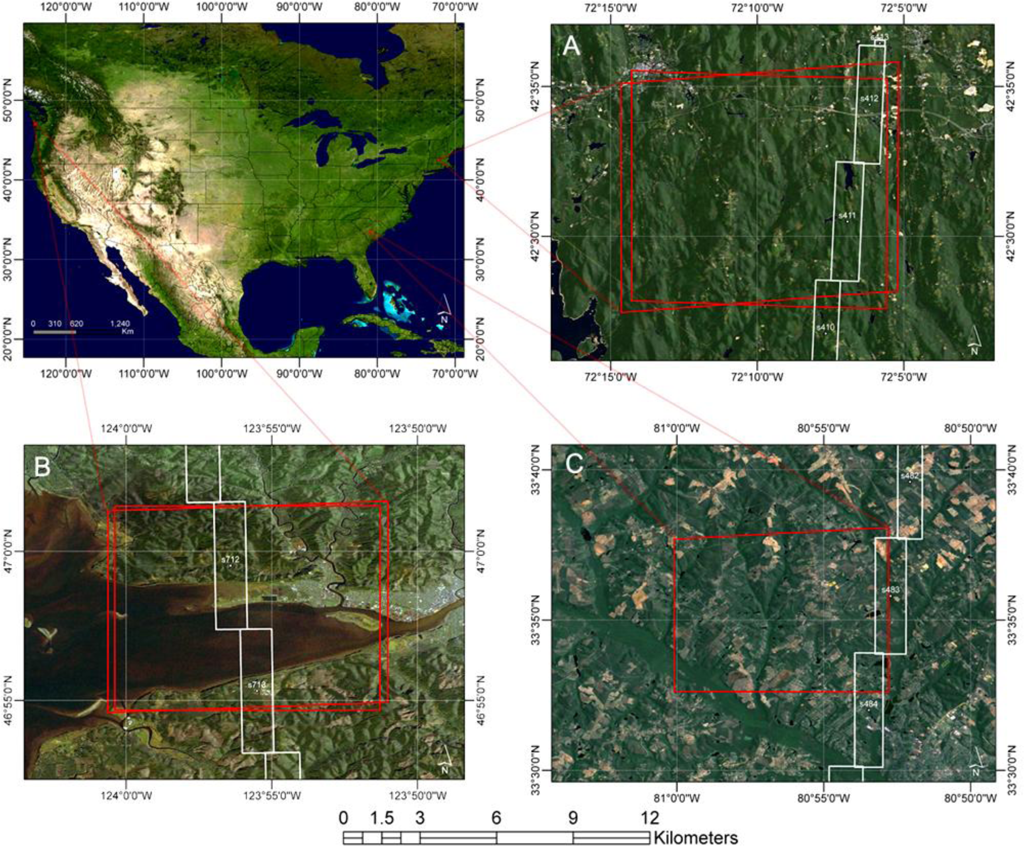
2. Study Areas
3. Data and Methods
3.1. G-LiHT Airborne Laser Scanner
3.2. IKONOS Stereo Imagery
3.3. NED DTMs
3.4. Processing Stereo HRSI
- (1)
- Stereo products were processed by using IDL/ENVI Version 5.0 DEM extraction module software. These data contain RPC files with geolocation information. DSMs were produced with RPCs alone and with GCPs to refine RPCs;
- (2)
- Identical features in each image pair were manually collected, generating fifty or more stereoscopic parallax tie points. Points were collected with an even distribution throughout the image overlap and they had a maximum y-parallax error of 0.75 m. Typically, man-made features (buildings, road intersections, parking lots, etc.) with easily identifiable corners or intersections were selected between images. Tie points were used to generate left and right epipolar images (stereo images that overlap, and when displayed together produce an anaglyph, or 3-D viewable image) that are useful for solving the external image orientation. By overlaying epipolar images, one can produce an anaglyph or 3-D image (with 3-D red/blue glasses) so that height through parallax can be extracted. Stereo tie points then guide a moving window to develop correlated tie points between epipolar images to produce posts of height or grid points in a TIN from which stereo DSMs are rasterized from. Using epipolar images reduces one dimension of variability and increases the processing speed of image matching. Images are matched through successive iterations starting at coarse pyramid levels that are predefined (starting at 264), moving downward with each successive TIN toward full resolution (128, 64, 32, 8, 4, 2, 1). User input cannot be provided with ENVI’s DEM extraction module through the matching procedure and no preprocessing filters were applied to optimize images for feature extraction;
- (3)
- GCPs were identified from bare areas in IKONOS and NED DTM data. GCPs were placed where identical image features existed between stereo pairs, and height was estimated from the same approximate location in the DTM. For each GCP the NED DTM height was recorded for IKONOS DSM processing. Locations were selected based on low topographic relief to reduce vertical error in the horizontal plane. We acknowledge that this process was straight forward and easily accomplished with LiDAR derived NED DTMs as similar features in IKONOS and NED are pronounced when comparing 3 m and 1 m data. This task was more difficult with NED 10 m DTM data as it has less pronounced features to select visually identifiable co-located points. Previous studies have reported large increases in accuracy in both vertical and horizontal error when using GCPs. A notable improvement of this approach is high-resolution DTMs (3-m) that enable the identification of similar features in stereo HRSI. This could result in a large cost savings and improve accuracy of CHMs compared to collecting in-situ GCPs;
- (4)
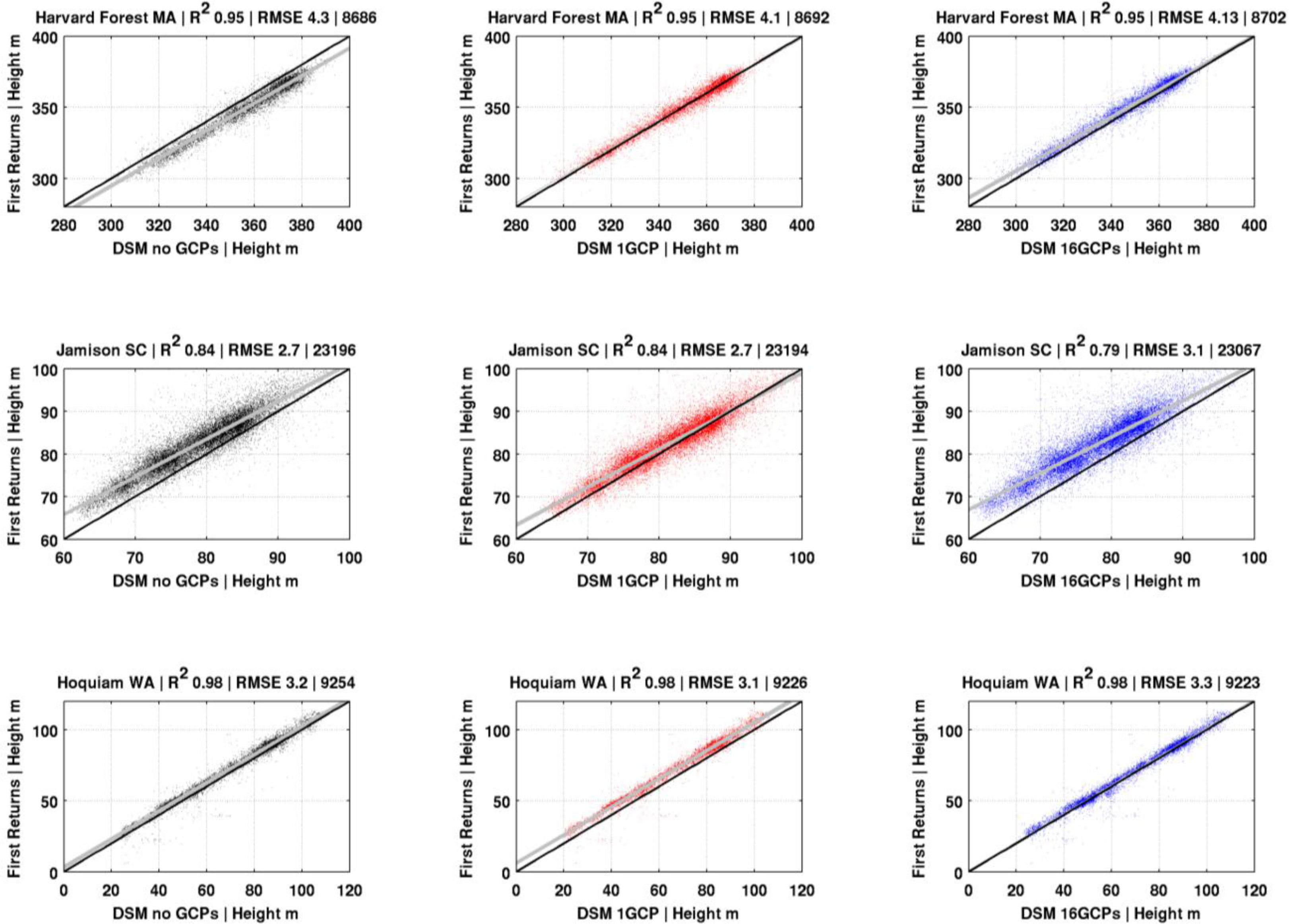
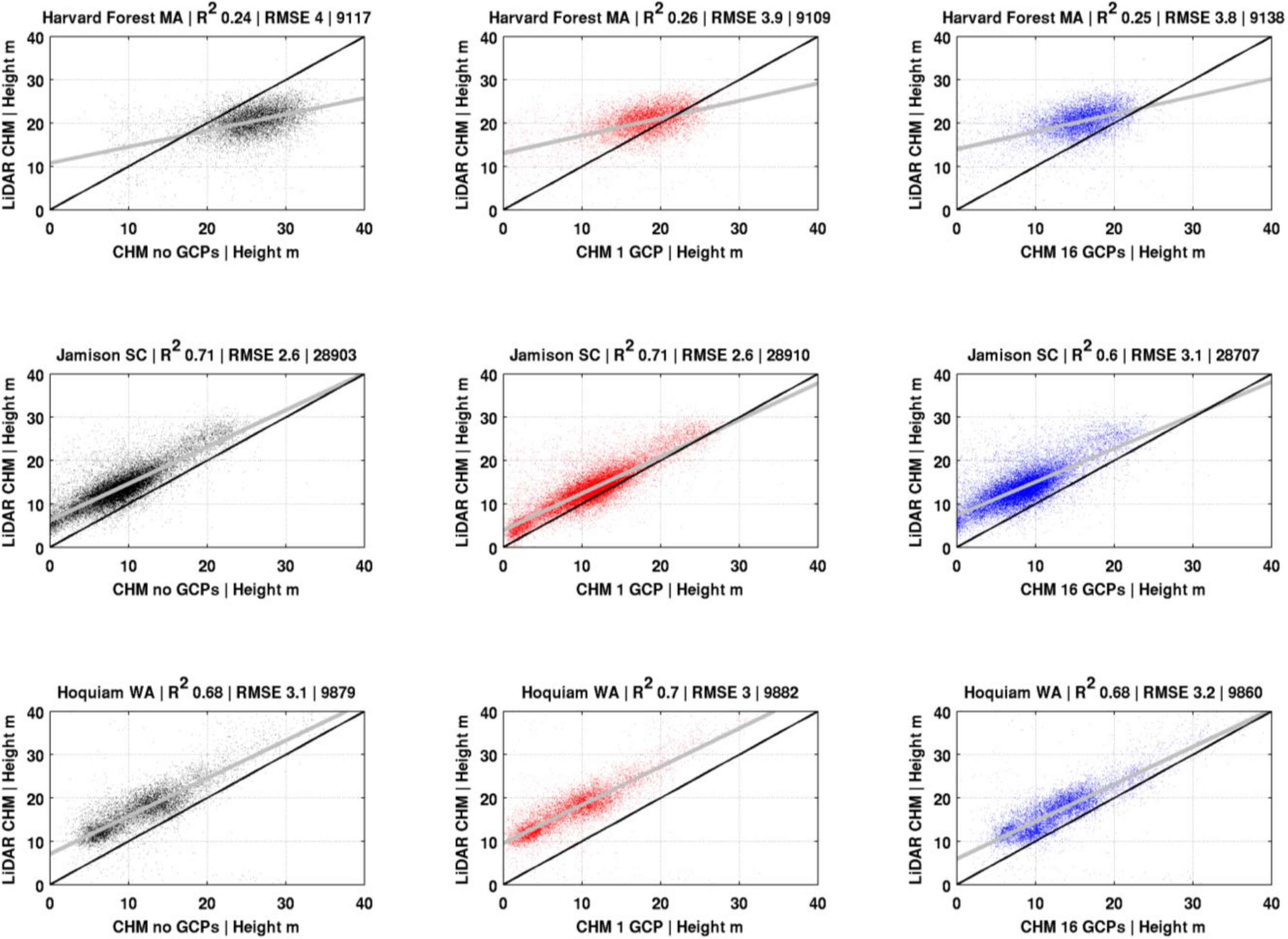
- GCPs were then used to improve pixel to ground relationships in building epipolar images for image correlation analysis in development of DSMs. We produced three types of DSMs from the IKONOS Geo stereo data to understand and quantify errors in stereo CHM development. These included: (a) DSMs based on RPCs alone, requiring a geoid calculation; (b) DSMs derived with one GCP from NED DTM in a bare earth location; and (c) DSMs derived with 16 evenly distributed GCPs in bare earth locations throughout the image.
3.5. Valid Data Ranges
3.6. Data Comparison
4. Results
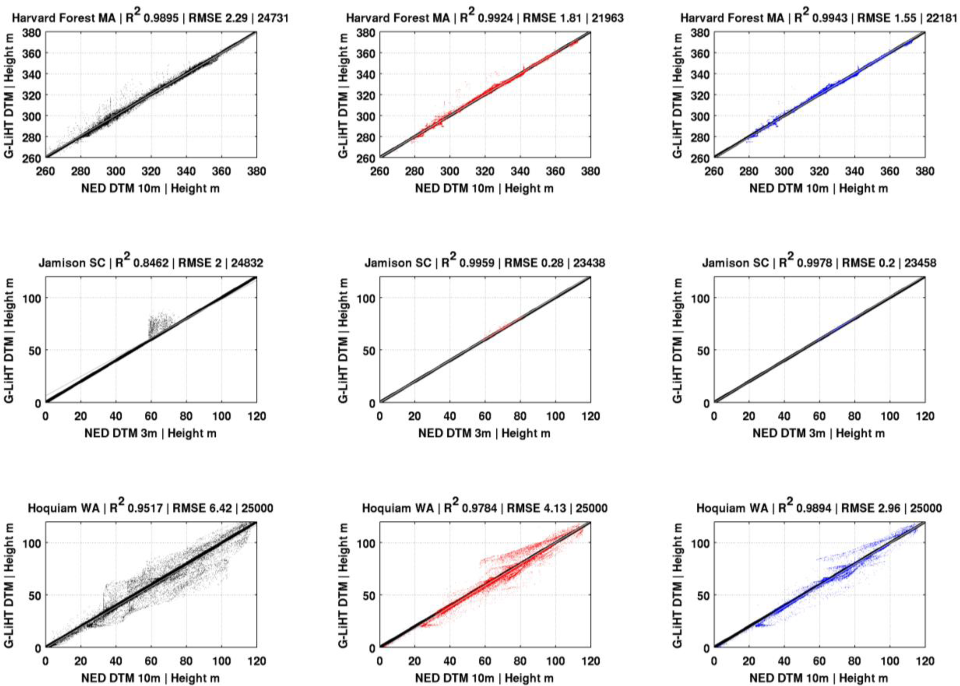
4.1. NED DTMs vs. G-LiHT DTMs
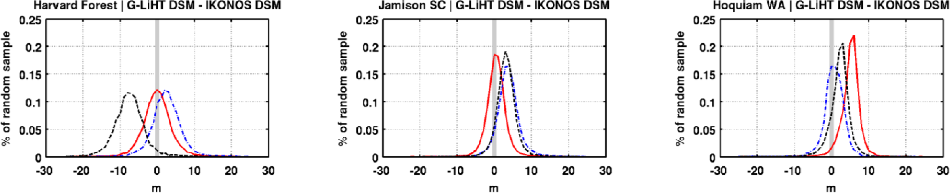
4.2. IKONOS DSMs vs. G-LiHT DSMs
4.3. IKONOS CHMs vs. G-LiHT CHMs
5. Discussion
6. Conclusions
Acknowledgments
Author Contributions
Conflict of Interest
References
- Gower, S.T. Patterns and mechanisms of the forest carbon cycle. Annu. Rev. Environ. Resour 2003, 28, 169–204. [Google Scholar]
- Knorr, W.; Quest, M.S. Global-scale drought caused atmospheric CO2 increase. EOS Trans 2005, 86, 178–181. [Google Scholar]
- Brovkin, V.; Sitch, S.; von Bloh, W.; Claussen, M.; Bauer, E.; Cramer, W. Role of land cover changes for atmospheric CO2 increase and climate change during the last 150 years. Glob. Chang. Biol 2004, 10, 1253–1266. [Google Scholar]
- Wulder, M.A.; White, J.C.; Stinson, G.; Hilker, T.; Kurz, W.A.; Coops, N.C.; St-Onge, B.; Trofymow, J.A. Implications of differing input data sources and approaches upon forest carbon stock estimation. Environ. Monit. Assess 2010, 166, 543–561. [Google Scholar]
- Vega, C.; St-Onge, B. Mapping site index and age by linking a time series of canopy height models with growth curves. For. Ecol. Manag 2009, 257, 951–959. [Google Scholar]
- Gao, J. Towards accurate determination of surface height using modern geoinformattic methods: Possibilities and limitations. Prog. Phys. Geogr 2007, 31, 591–605. [Google Scholar]
- Toutin, T. DTM generation from Ikonos in-track stereo images using a 3D physical model. Photogramm. Eng. Remote Sens 2004, 70, 695–702. [Google Scholar]
- Wang, J.; Di, K.C.; Li, R. Evaluation and improvement of geopositioning accuracy of IKONOS stereo imagery. J. Surv. Eng.-Asce 2005, 131, 35–42. [Google Scholar]
- St-Onge, B.; Hu, Y.; Vega, C. Mapping the height and above-ground biomass of a mixed forest using lidar and stereo Ikonos images. Int. J. Remote Sens 2008, 29, 1277–1294. [Google Scholar]
- Vega, C.; St-Onge, B. Height growth reconstruction of a boreal forest canopy over a period of 58 years using a combination of photogrammetric and lidar models. Remote Sens. Environ 2008, 112, 1784–1794. [Google Scholar] [Green Version]
- Cook, B.D.; Corp, L.A.; Nelson, R.F.; Middleton, E.; Morton, D.C.; McCorkel, J.T.; Masek, J.G.; Ranson, J.; Ly, V.; Montesano, P. NASA Goddard’s LiDAR, hyperspectral anad thermal (G-LiHT) airborne imager. Remote Sens 2013, 5, 4045–4066. [Google Scholar]
- The Forest Inventory and Analysis (FIA). United States Forest Service Forest Inventory and Analysis National Program. Available online: http://fia.fs.fed.us/ (accessed on 22 January 2014).
- Masek, J.G.; Cohen, W.B.; Leckie, D.; Wulder, M.A.; Vargas, R.; de Jong, B.; Healey, S.; Law, B.; Birdsey, R.; Houghton, R.A.; et al. Recent rates of forest harvest and conversion in North America. J. Geophys. Res. Biogeosci 2011, 116. [Google Scholar] [CrossRef]
- Neigh, C.S.R.; Masek, J.G.; Nickeson, J. High-resolution satellite data open for government research. EOS Trans 2013, 94, 121–123. [Google Scholar]
- Falkowski, M.J.; Wulder, M.A.; White, J.C.; Gillis, M.D. Supporting large-area, sample-based forest inventories with very high spatial resolution satellite imagery. Prog. Phys. Geogr 2009, 33, 403–423. [Google Scholar]
- Waser, L.T.; Baltsavias, E.; Ecker, K.; Eisenbeiss, H.; Ginzler, C.; Kuchler, M.; Thee, P.; Zhang, L. High-resolution digital surface models (DSMs) for modelling fractional shrub/tree cover in a mire environment. Int. J. Remote Sens 2008, 29, 1261–1276. [Google Scholar]
- Betts, H.D.; Brown, L.J.; Stewart, G.H. Forest canopy gap detection and characterisation by the use of high-resolution digital elevation models. N. Zeal. J. Ecol 2005, 29, 95–103. [Google Scholar]
- Wallerman, J.; Bohlin, J.; Fransson, J.E.S. Forest Height Estimation Using Semi-Individual Tree Detection in Multi-Spectral 3D Aerial DMC Data. Proceedings of the 2012 IEEE International Conference on Geoscience and Remote Sensing Symposium (IGARSS), Munich, Gremany, 22–27 July 2012; pp. 6372–6375.
- Itaya, A.; Miura, M.; Yamamoto, S.I. Canopy height changes of an old-growth evergreen broad-leaved forest analyzed with digital elevation models. For. Ecol. Manag 2004, 194, 403–411. [Google Scholar]
- Katsch, C.; Stocker, M. Automatic determination of stand heights from aerial photography using digital photogrammetric systems. Allg. Forst und Jagdztg 2000, 171, 74–80. [Google Scholar]
- Bohlin, J.; Wallerman, J.; Fransson, J.E.S. Forest variable estimation using photogrammetric matching of digital aerial images in combination with a high-resolution DEM. Scand. J. For. Res 2012, 27, 692–699. [Google Scholar]
- Gong, P.; Sheng, Y.; Biging, G.S. 3D model-based tree measurement from high-resolution aerial imagery. Photogramm. Eng. Remote Sens 2002, 68, 1203–1212. [Google Scholar]
- Poon, J.; Fraser, C.S.; Zhang, C.S.; Li, Z.; Gruen, A. Quality assessment of digital surface models generated from IKONOS imagery. Photogramm. Rec 2005, 20, 162–171. [Google Scholar]
- Ni, W.J.; Guo, Z.F.; Zhang, Z.Y.; Sun, G.Q.; Huang, W.L. Semi-Automatic Extraction of Digital Surface Model Using Alos/Prism Data with ENVI. Proceedings of the 2012 IEEE International Conference on Geoscience and Remote Sensing Symposium (IGARSS), Munich, Gremany, 22–27 July 2012; pp. 6557–6560.
- Takahashi, M.; Shimada, M.; Tadono, T.; Watanabe, M. Calculation of Trees Height Using PRISM-DSM. Proceedings of the 2012 IEEE International Conference on Geoscience and Remote Sensing Symposium (IGARSS), Munich, Gremany, 22–27 July 2012; pp. 6495–6498.
- Baltsavias, E.; Gruen, A.; Eisenbeiss, H.; Zhang, L.; Waser, L.T. High-quality image matching and automated generation of 3D tree models. Int. J. Remote Sens 2008, 29, 1243–1259. [Google Scholar]
- Alobeid, A.; Jacobsen, K.; Heipke, C. Comparison of matching algorithms for DSM generation in urban areas from Ikonos imagery. Photogramm. Eng. Remote Sens 2010, 76, 1041–1050. [Google Scholar]
- Xiong, Z.; Zhang, Y. Automatic 3D building extraction from stereo IKONOS images. Int. Geosci. Remote Sens 2006, 3283–3286. [Google Scholar]
- Eckert, S.; Hollands, T. Comparison of automatic DSM generation modules by processing IKONOS stereo data of an urban area. IEEE J.-Stars 2010, 3, 162–167. [Google Scholar]
- Hirschmuller, H.; Scholten, F.; Hirzinger, G. Stereo vision based reconstruction of huge urban areas from an airborne pushbroom camera (HRSC). Pattern Recognit 2005, 3663, 58–66. [Google Scholar]
- Fraser, C.S.; Yamakawa, T.; Hanley, H.B.; Dare, P.M. Geopositioning from High-Resolution Satellite Imagery: Experiences with the Affine Sensor Orientation Model. Proceedings of the 2003 IEEE International Conference on Geoscience and Remote Sensing Symposium (IGARSS), Toulouse, France, 21–25 July 2003; 5, pp. 3002–3004.
- St-Onge, B.; Vega, C.; Fournier, R.A.; Hu, Y. Mapping canopy height using a combination of digital stereo-photogrammetry and lidar. Int. J. Remote Sens 2008, 29, 3343–3364. [Google Scholar]
- Cook, B. G-LiHT: Goddard’s LiDAR, Hyperspectral & Thermal Imager. Available online: http://gliht.gsfc.nasa.gov/ (accessed on 22 January 2014).
- Zhang, K.Q.; Chen, S.C.; Whitman, D.; Shyu, M.L.; Yan, J.H.; Zhang, C.C. A progressive morphological filter for removing non-ground measurements from airborne LiDAR data. IEEE Trans. Geosci. Remote Sens 2003, 41, 872–882. [Google Scholar]
- USGS. USGS Commercial Remote Sensing Space Policy (CRSSP) Imagery-Derived Requirements (CIDR) Tool. Available online: https://cidr.cr.usgs.gov (accessed on 22 January 2014).
- Fraser, C.S.; Dial, G.; Grodecki, J. Sensor orientation via RPCs. ISPRS J. Photogramm 2006, 60, 182–194. [Google Scholar]
- Fraser, C.S.; Hanley, H.B. Bias-compensated RPCs for sensor orientation of high-resolution satellite imagery. Photogramm. Eng. Remote Sens 2005, 71, 909–915. [Google Scholar]
- USGS National Elevation Dataset. Available online: http://ned.usgs.gov/ (accessed on 22 January 2014).
- Gesch, D.; Oimoen, M.; Greenlee, S.; Nelson, C.; Steuck, M.; Tyler, D. The national elevation dataset. Photogramm. Eng. Remote Sens 2002, 68, 5–11. [Google Scholar]
- Gesch, D.B. The National Elevation Dataset. In Digital Elevation Model Technologies and Applications: The DEM Users Manual, 2nd ed; American Society of Photogrammetry and Remote Sensing: Bethesda, MD, USA, 2007; pp. 99–118. [Google Scholar]
- Huang, C.; Goward, S.N.; Masek, J.G.; Thomas, N.; Zhu, Z.L.; Vogelmann, J.E. An automated apporach for reconstructing recent forest disturbance history using dense Landsat time series stacks. Remote Sens. Environ 2010, 114, 183–198. [Google Scholar]
- Masek, J.G.; Goward, S.N.; Kennedy, R.E.; Cohen, W.B.; Moisen, G.G.; Schleewies, K.; Huang, C. United States forest disturbance trends observed using Landsat time series. Ecosystems 2013, 16, 1087–1104. [Google Scholar]
- Goward, S.N.; Masek, J.G.; Cohen, W.; Moisen, G.; Collatz, G.J.; Healey, S.; Houghton, R.; Huang, C.; Kennedy, R.; Law, B.; et al. Forest disturbance and North American carbon flux. EOS Trans 2008, 89, 105–116. [Google Scholar]
- Jenkins, J.C.; Chojnacky, D.C.; Heath, L.S.; Birdsey, R.A. National-scale biomass estimators for United States tree species. For. Sci 2003, 49, 12–35. [Google Scholar]
- Shugart, H.H.; Saatchi, S.; Hall, F.G. Importance of structure and its measurement in quantifying function of forest ecosystems. J. Geophys. Res. Biogeosci 2010, 115. [Google Scholar] [CrossRef]
- Harvard, U. Harvard Forest. Available online: http://harvardforest.fas.harvard.edu/hf011-hurricane-maps (accessed on 22 January 2014).
- Ranson, K.J.; Nelson, R.; Kimes, D.; Kharuk, V.; Sun, G.; Montesano, P. Using MODIS and GLAS Data to Develop Timber Volume Estimates in Central Siberia. Proceedings of the 2007 IEEE International Conference on Geoscience and Remote Sensing Symposium (IGARSS), Barcelona, Spain, 23–28 July 2007; pp. 2306–2309.
- Neigh, C.S.R.; Nelson, R.F.; Ranson, K.J.; Margolis, H.A.; Montesano, P.M.; Sun, G.Q.; Kharuk, V.; Næsset, E.; Wulder, M.A.; Andersen, H.E. Taking stock of circumboreal forest carbon with ground measurements, airborne and spaceborne LiDAR. Remote Sens. Environ 2013, 137, 274–287. [Google Scholar]
- Nelson, R.; Ranson, K.J.; Sun, G.; Kimes, D.S.; Kharuk, V.; Montesano, P. Estimating Siberian timber volume using MODIS and ICESat/GLAS. Remote Sens. Environ 2009, 113, 691–701. [Google Scholar]
- Blackard, J.A.; Finco, M.V.; Helmer, E.H.; Holden, G.R.; Hoppus, M.L.; Jacobs, D.M.; Lister, A.J.; Moisen, G.G.; Nelson, M.D.; Riemann, R.; et al. Mapping US forest biomass using nationwide forest inventory data and moderate resolution information. Remote Sens. Environ 2008, 112, 1658–1677. [Google Scholar]
- Saatchi, S.S.; Houghton, R.A.; Alvala, R.; Soares, J.V.; Yu, Y. Distribution of aboveground live biomass in the Amazon basin. Glob. Chang. Biol 2007, 13, 816–837. [Google Scholar]
- Baccini, A.; Goetz, S.J.; Walker, W.S.; Laporte, N.T.; Sun, M.; Sulla-Menashe, D.; Hackler, J.; Beck, P.S.A.; Dubayah, R.; Friedl, M.A.; et al. Estimated carbon dioxide emissions from tropical deforestation improved by carbon-density maps. Nat. Clim. Chang 2012, 2, 182–185. [Google Scholar]
- Stennett, T.A.; Wade-Grusky, S. Lidar Fact and Fiction. Available online: http://www.profsurv.com/magazine/article.aspx?i=2110 (accessed on 22 January 2014).


| Study Region | G-LiHT Acquisition Date mm/yr | G-LiHT Data ID | IKONOS Acquisition Date mm/dd/yr | IKONOS Nominal Collection Elevation | B/H Ratio | NED DTM Resolution (m) |
|---|---|---|---|---|---|---|
| Harvard Forest MA | 08/2011 | AMIGACarb_5S_Aug2011 | 10/12/2000 | 64.40°–72.87° | 0.64 | 10 |
| Jamison SC | 09/2011 | AMIGACarb_13s_Sep2011 | 10/31/2010 | 60.75°–87.04° | 0.55 | 3 |
| Hoquiam WA | 08/2012 | AMIGACarb_G03_Aug2012 | 09/14/2008 | 69.03°–77.94° | 0.58 | 10 |
| Valid Range | |
|---|---|
| CHM height | >0.1 m |
| DSM height | 0 > 500 m |
| DTM height * | 0 > 500 m |
| IKONOS NDVI | >0.3 |
| G-LiHT instrument calibrated apparent reflectance first returns | <0.15 |
| G-LiHT instrument calibrated apparent reflectance last returns * | >0.35 |
| G-LiHT DTM Slope * | <10° |
| G-LiHT and IKONOS DSM 5 pixel sample | <2 standard deviations |
| Landsat VCT | All data pre and non disturbed forest post IKONOS acquisition. |
| Harvard Forest—Massachusetts | ||||
| Elev | Error X | Error Y | Error Z | |
| Median | 320.0 | 0.00003 | 0.00011 | 18.26 |
| Minimum | 231.9 | −0.00006 | −0.00015 | 12.47 |
| Maximum | 353.8 | 0.00032 | 0.00021 | 22.84 |
| Standard Deviation | 34.4 | 0.00008 | 0.00010 | 2.39 |
| Jamison—South Carolina | ||||
| Elev | Error X | Error Y | Error Z | |
| Median | 84.2 | 0.25675 | 2.83890 | 33.00 |
| Minimum | 55.0 | −1.62250 | −3.95360 | 18.81 |
| Maximum | 103.5 | 2.50230 | 37.50100 | 40.16 |
| Standard Deviation | 11.6 | 0.98625 | 9.20157 | 4.85 |
| Hoquiam—Washington | ||||
| Elev | Error X | Error Y | Error Z | |
| Median | 40.9 | −0.00001 | 0.00001 | 25.30 |
| Minimum | 2.8 | −0.00048 | −0.00015 | 22.81 |
| Maximum | 99.4 | 0.00004 | 0.00010 | 28.52 |
| Standard Deviation | 30.9 | 0.00012 | 0.00008 | 1.65 |
© 2014 by the authors; licensee MDPI, Basel, Switzerland This article is an open access article distributed under the terms and conditions of the Creative Commons Attribution license (http://creativecommons.org/licenses/by/3.0/).
Share and Cite
Neigh, C.S.R.; Masek, J.G.; Bourget, P.; Cook, B.; Huang, C.; Rishmawi, K.; Zhao, F. Deciphering the Precision of Stereo IKONOS Canopy Height Models for US Forests with G-LiHT Airborne LiDAR. Remote Sens. 2014, 6, 1762-1782. https://doi.org/10.3390/rs6031762
Neigh CSR, Masek JG, Bourget P, Cook B, Huang C, Rishmawi K, Zhao F. Deciphering the Precision of Stereo IKONOS Canopy Height Models for US Forests with G-LiHT Airborne LiDAR. Remote Sensing. 2014; 6(3):1762-1782. https://doi.org/10.3390/rs6031762
Chicago/Turabian StyleNeigh, Christopher S. R., Jeffrey G. Masek, Paul Bourget, Bruce Cook, Chengquan Huang, Khaldoun Rishmawi, and Feng Zhao. 2014. "Deciphering the Precision of Stereo IKONOS Canopy Height Models for US Forests with G-LiHT Airborne LiDAR" Remote Sensing 6, no. 3: 1762-1782. https://doi.org/10.3390/rs6031762