Evaluation of Multiple Spring Phenological Indicators of Yearly GPP and NEP at Three Canadian Forest Sites

Abstract

Phenological shifts in events such as flowering and bud break are important indicators of ecosystem processes, and are therefore of particular significance for carbon (C) cycle research. Using long-term flux data from three contrasting plant functional type (evergreen and deciduous) boreal forest sites, we evaluated and compared the responses of annual C fluxes to multiple spring phenological indicators, including the C-uptake period onset (CUP onset), spring temperature (average value from March to May), and satellite-derived enhanced vegetation index (EVI) (average value from March to May). We found that the CUP onset was negatively correlated with annual gross primary production (GPP) for all three sites, but that its predictive strength for annual net ecosystem production (NEP) differed substantially among plant functional types. Spring temperature demonstrated particularly good potential for predicting both annual GPP and NEP for the evergreen sites, but not for the deciduous site. Spring EVI was demonstrated to have potential for predicting annual NEP for all sites. However, both plant functional types confounded the correlation of annual NEP with annual GPP. Although none of these phenological indicators provided consistent insight into annual C fluxes, using various currently available datasets our results remain potentially useful for the assessment of forest C cycling with future climate change. Previous analyses using only a single phenological metric should be considered with caution.

1. Introduction

The timing of plant canopy phenological events is an important indicator of the temporal and spatial variability of ecosystem-atmosphere fluxes [1,2]. Therefore, efforts have focused on understanding the impacts of phenological transitions on carbon (C) sequestration both at the plot level and on a continental scale [3–5].

Interannual variability of net ecosystem production (NEP), the difference between gross primary production (GPP) and ecosystem respiration (R_e), is regulated by both biotic (e.g., GPP, stand age) and abiotic (e.g., precipitation, temperature) variables [6,7]. However, annual NEP is also dependent on the seasonal variation of other variables, such as spring temperature and growing season length (GSL) [8–12]. Higher spring temperatures tend to increase annual NEP in various ecosystems, likely due to the earlier onset of canopy greenness [13,14]. In contrast, autumn warming would have a negative influence on annual NEP if ecosystem respiration rates were more sensitive to temperature changes [15,16]. These results imply that seasonal changes in climate are important indicators of the annual NEP, as these changes can shift phenological transitions and consequently affect plant growth rhythm.

Various phenological indicators derived from diverse datasets have been used in previous studies. Among these, carbon flux-based phenology (CFP) has recently been used widely. These phenological indicators include the onset and end of the carbon-uptake period (CUP) (i.e., the period of net carbon uptake from the atmosphere) [1,2,9,17–20]. Spring temperature (mean values from March to May) has also been used to indicate the onset of the growing season and the annual NEP [3,13]. However, flux-based phenology is limited by the availability of flux data (i.e., spatial representativeness), as well as the distributions and footprints of the towers [17]. Although many flux networks, such as AmeriFlux and Fluxnet-Canada, have been established, data from these networks provide critically useful but spatially limited information for global applications.

Satellite data have been utilized as an alternative for the capture of phenological transitions at regional, continental, and global scales [20]. Fitted curves for vegetation index (VI) time series are used (e.g., determining the transition dates from the local maxima and minima in the fitted function), including the enhanced vegetation index (EVI) [4,18,21], the normalized difference vegetation index (NDVI) [2,20,22], and the MERIS Terrestrial Chlorophyll Index (MTCI) [23]. The advantage of remote-sensing data is that they are uniquely spatially explicit, and are useful for evaluating and validating models and assumptions with a wider spatial coverage compared to flux measurements. Furthermore, the results presented by Fisher and Mustard [24] indicate a good general consensus among different spatial datasets of satellite-generated interannual phenology features, supporting the effectiveness of remote-sensing data for monitoring forest responses to global-scale climate variability [25].

As demonstrated by Garrity et al. [4], the relative strengths and weaknesses of phenological indicators must be identified and compared. This is a necessary step for the incorporation of these indicators into ecosystem models, to better interpret annual C fluxes. Furthermore, it is vital to understand the effects of plant functional types on the relationship between C fluxes and phenological indicators, which is significant when scaling up these relationships. Here we present a comparison of the predictive strength of several spring phenological indicators for annual GPP and NEP in boreal regions of Canada, where climate warming has been suggested to be the greatest worldwide during the several past decades [14]. Long-term flux measurements at three forest sites (one deciduous and two evergreen stands), as well as a time series of satellite observations were used to analyze the responses of annual NEP and GPP to multiple spring phenological indicators, including C-uptake period onset, spring temperature, and spring EVI. The main objectives of this study were: (1) to compare the potential of various spring phenological indicators for predicting annual C fluxes, and (2) to analyze the responses of different plant functional types to the relationship between C fluxes and these spring phenological indicators.

2. Materials and Methods

2.1. Study Sites

Three boreal forests sites were selected for this analysis. The first was the 84-year-old aspen site (SK-OA, established 1919, 53.63°N, −106.20°E, 2001–2009), located within the southern boundary of Prince Albert National Park, ∼50 km from Prince Albert, Canada [26,27]. This site consists largely of trembling aspen (Populus tremuloides Michx.), with intermittent occurrences of balsam poplar (Populus balsamifera L.). The continuous understory, which reaches a mean height of 1.5–2.0 m, is composed of hazelnut (Corylus cornuta Marsh), and to a lesser extent wild rose (Rosa woodsii), willow (Salix spp.), alder (Alnus crispa), and a variety of grasses and herbs. The soil in the area is an Orthic Gray Luvisol that is well- to moderately well-drained, with a loam to clay loam texture. The stand density is ∼980 trees ha⁻¹, with a mean tree height of 20.1 m and an average diameter at breast height (DBH) of 20.5 cm.

The second site was an old black spruce site (SK-OBS, established 1894, 53.98°N, −105.12°W, 2001–2009) located in the mid-boreal lowland ecoregion in the boreal plain ecozone near Prince Albert, Canada. The dominant species is black spruce (Picea mariana Mill.), with scattered jack pine (Pinus banksiana Lamb.) and tamarack (Larix laricina DuRoi.). The understory is primarily wild rose and Labrador tea (Ledum groenlandieum), with a groundcover of Sphagnum spp. in wetter areas, and feather mosses (Pleurozium schreberi) and lichens (Claudina sp.) in drier areas. The soil in the area is a Gleyed Eluviated Eutric Brunisol (Peaty Phase) with imperfect to poor drainage, a 20–30 cm forest floor, and a sandy loam to loam texture developed from thick glacial deposits [26]. The stand density is ∼4330 trees ha⁻¹, with a mean tree height of 7.2 m and an average DBH of 7.1 cm.

The third site was an old jack pine stand (SK-OJP, established 1929, 53.92°N, −104.69°W, 2001–2009). The dominant species at this site is jack pine, with a sparse understory of isolated alder clumps and a ground cover of bearberry (Arctostaphylos uva-ursi), lichens, and grasses. The soil in the area is an Orthic Eutric Brunisol with very good drainage and a fine sand texture. The stand density is 1320 trees ha⁻¹, with a mean tree height of 12.7 m and an average DBH of 12.9 cm [27].

2.2. Flux Data

Flux data provide continuous net ecosystem exchange (NEE) measurements, assisting with the mechanistic understanding of temporal and spatial variations of C fluxes [17,28]. Fluxes of momentum, sensible heat, water vapor, and CO₂ were measured using the eddy covariance (EC) technique [26]. Velocity components, air temperature, water vapor density, and CO₂ concentration in the air were sampled rapidly, and calculations of relevant covariances were performed from these samples to obtain the fluxes. Wind speed and CO₂ mixing ratio were measured at a specific height above the ground (i.e., 39 m for SK-OA and 25 m for SK-OBS) using a three dimensional sonic anemometer-thermometer (SAT, Model R3, Gill Instruments, Lymington, UK) and a closed-path infrared gas analyzer (IRGA) (Model LI-6262), respectively.

A standard procedure implemented by Fluxnet-Canada was used to estimate the annual NEP for model evaluation. NEP was partitioned into GPP and R_e using gap-filled half-hourly measurements of NEE. Empirical regressions of nighttime NEE versus temperature and daytime GPP versus photosynthetic active radiation (PAR) were used to estimate R_e and GPP, respectively, and gaps were filled as described by Barr et al. [26]. Three steps were followed to acquire the annual NEP, GPP, and R_e. First, the net ecosystem exchange (NEE) was estimated as the sum of the measured eddy and air-column storage fluxes with two adjustments. The first is a correction for low turbulence, where a critical value of friction velocity (u*) is used to filter unacceptable data. Typically values of u* > 0.35 m·s⁻¹ were employed, with individual values determined for each site. The second adjustment was for poor energy-balance-closure, where turbulent fluxes (including NEP) were adjusted so that the sum of sensible and latent heat fluxes balanced the net radiation minus energy storage terms. Next, measured R_e was estimated as R_e = −NEP during periods when GPP was known to be zero, specifically at night and during both night and day in the cold season (periods when both air (T_a) and 2-cm soil (T_s) temperatures were below 0 °C). Finally, GPP was estimated as NEP + R_e (daytime) or zero (nighttime and during periods when both T_a and T_s were less than 0 °C) with an additional empirical model to fit the non-zero GPP data for the entire year.

2.3. Satellite Data

Satellite-based observations from the Moderate Resolution Imaging Spectroradiometer (MODIS) sensor were used in this study. We used the MODIS land surface vegetation index product, which was downloaded from the Oak Ridge National Laboratory’s Distributed Active Archive Center (DAAC) website [29]. This MODIS vegetation index product (MOD13Q1, 500 m, collection 5) can provide the enhanced vegetation index (EVI) [30] for a 16-day time interval using atmospherically corrected bi-directional surface reflectance. Low-quality observations resulting from cloud contamination and other factors (e.g., snow) were rejected by selecting the quality flag, which ensured that the monthly EVO calculation was of good quality.

The EVI was quantified by the following equation:

$$\mathit{EVI}=2.5\times \frac{R_{\mathit{NIR}}-R_{\mathit{Red}}}{1+R_{\mathit{NIR}}+6\times R_{\mathit{Red}}-7.5\times R_{\mathit{Blue}}}$$

(1)

where R_NIR, R_Red, and R_Blue represent the reflectance at near-infrared, red, and blue wavelengths (nm), respectively. Based on the geo-location information (latitude and longitude) of the flux tower sites, EVI was extracted from the 3 × 3-pixel area at the center point on the flux tower, similar to the approaches of Sims et al. [31] and Wu et al. [32]. This was reasonable due to the large footprints (>1.5 km) of all sites throughout the year reported by Chen et al. [33]. The averages of the observations during the month were then used to represent the mean monthly value [34].

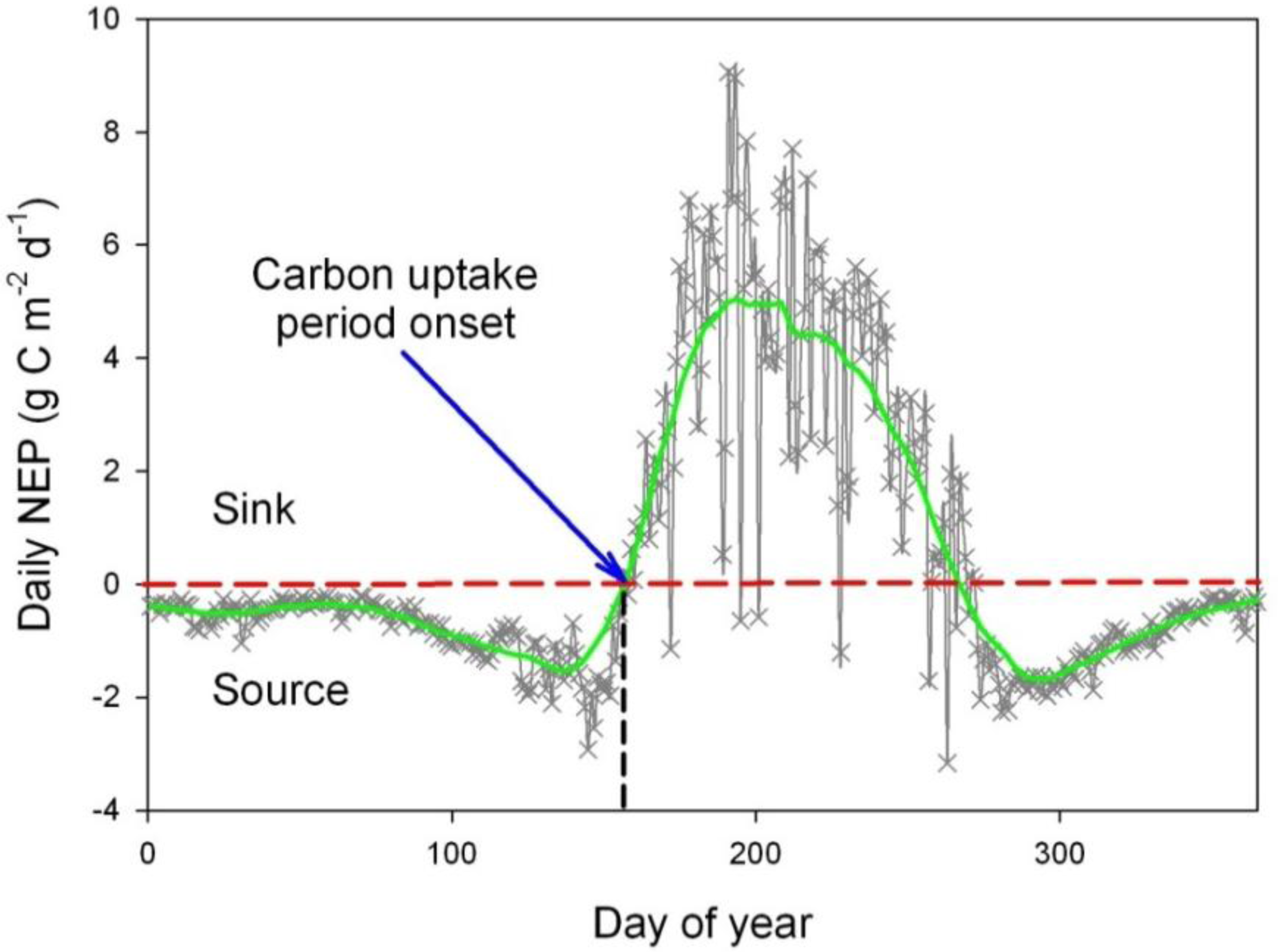
2.4. Spring Phenological Indicators

Three spring phenological indicators were used, i.e., the CUP onset, spring temperature (mean value of monthly data from March to May), and the spring EVI (mean value of monthly data from March to May). The method used to determine the CUP onset (day of year, DOY) from the daily NEP is shown in Figure 1. We first generated daily NEP over the whole year from the half-hourly measurements. Then, a negative exponential model using polynomial regression and weights computed from the Gaussian density function was adopted to derive the smoothed curve for daily NEP observations [5]. The CUP onset was designated as the first day when a positive daily NEP of the smoothed curve was observed.

3. Results

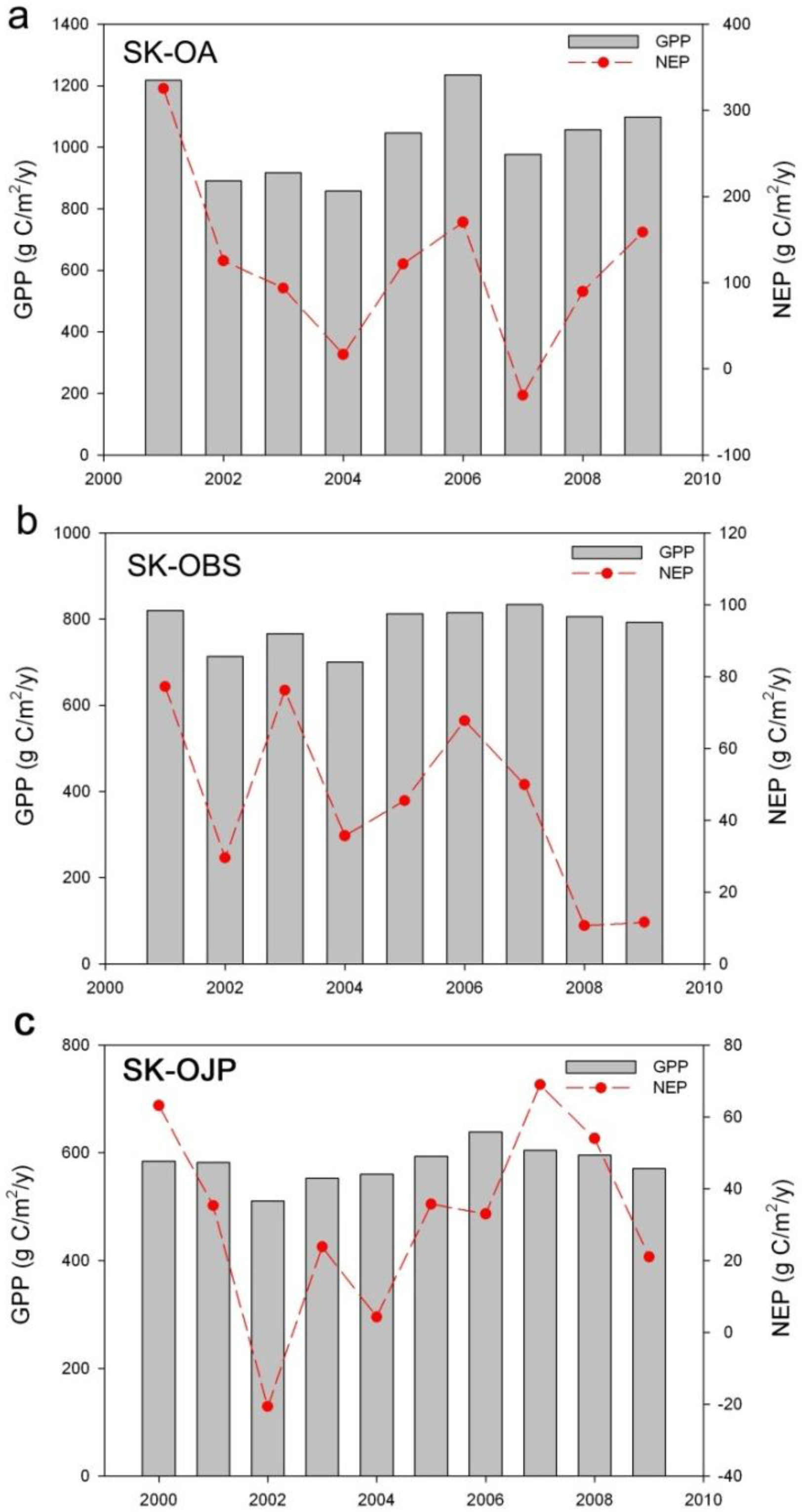
3.1. Descriptions of Annual C Fluxes

Annual ecosystem C fluxes, GPP, and NEP of all sites are shown in Figure 2. SK-OA, a deciduous site, showed high annual GPP with an average value of 1032 g·C·m⁻²·y⁻¹ for all observations over the 9 years. The NEP of this site fluctuated from −30 g·C·m⁻²·y⁻¹ in 2007 to the highest value of 325 g·C·m⁻²·y⁻¹ in 2001. The evergreen site, SK-OBS, had a lower annual GPP than SK-OA, with a value of 784 g·C·m⁻²·y⁻¹. The NEP of this site (45 g·C·m⁻²·y⁻¹) was also lower than that of SK-OA (119 g·C·m⁻²·y⁻¹). Similar results were found for the SK-OJP site, with annual GPP of 510–638 g·C·m⁻²·y⁻¹, and annual NEP between −20–68 g·C·m⁻²·y⁻¹. Another difference among these sites was the interannual variability in the C flux. The SK-OA site had a higher coefficient of variation (CV) in GPP (13%) than the two evergreen sites (6.1% for SK-OBS, and 5.9% for SK-OJP). However, all sites showed great interannual variability in annual NEP (84.6% for SK-OA, 56.7% for SK-OBS, and 84.7% for SK-OJP).

3.2. Spring Phenological Indicators across Sites and Intercorrelations among These Indicators

Comparisons among these spring phenological indicators were conducted for all sites (

Table 1. Comparison of the three phenological indicators for all sites in this study.

Sites		CUP Onset (DOY)	Ta_Spring (°C)	EVI_Spring
SK-OA	Minimum	132	−2.5	0.291
	Maximum	161	3.8	0.422
	Average	145	1.6	0.331
	SD	9.0	2.0	0.051
SK-OBS	Minimum	90	−3.2	0.232
	Maximum	120	3.3	0.263
	Average	106	0.7	0.245
	SD	10.6	2.1	0.012
SK-OJP	Minimum	95	−2.7	0.225
	Maximum	124	3.9	0.254
	Average	108	1.4	0.237
	SD	9.7	2.0	0.011

Note: DOY and SD represent day of year and standard deviation, respectively.

). Both CUP onset and spring EVI exhibited substantial variation among the sites, whereas the spring temperature range was similar at the three sites. Differences due to site characteristics could account for the observed variation in CUP onset and spring EVI. The deciduous forest site, SK-OA, showed a delayed CUP onset, with the earliest value at DOY 132 in 2001 and the latest at DOY 161 in 2004. The averages of the CUP onsets indicated that the two evergreen sites generally began net C uptake 40 days earlier than the SK-OA site. These two sites were also found to have greater interannual variability in CUP onset than the deciduous site, as indicated by the higher standard deviations. Statistical analysis indicated that the spring EVI of SK-OA was significantly higher (p < 0.001) than that of the SK-OBS and SK-OJP sites, which is reasonable given that evergreen species often demonstrate limited variability in interannual canopy greenness.

We further analyzed the correlations among these three spring phenological indicators for all sites (Figure 3). The results showed a correlation among all of the indicators, except between the spring EVI and CUP onset at the SK-OJP site. While spring temperature was moderately correlated with spring EVI, CUP onset was more strongly correlated with spring EVI, with R² values of 0.64 (p = 0.009) and 0.66 (p = 0.007) for SK-OA and SK-OBS, respectively. As CUP transitions play an important role in controlling annual C fluxes [1], we suggest that spring EVI is a candidate for incorporation into ecosystem models.

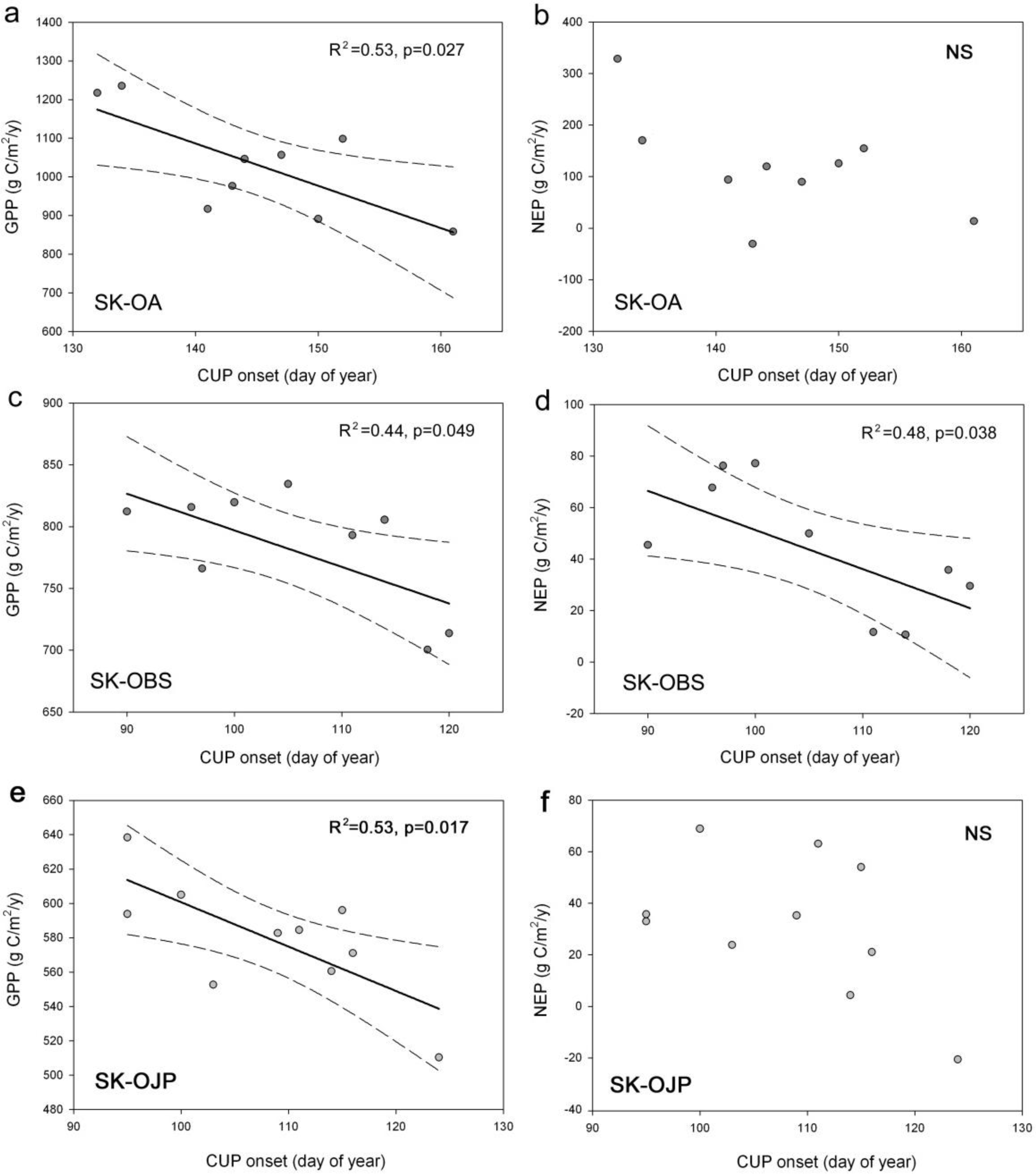
3.3. Relationships between CUP Onset and C Fluxes

The CUP onset was negatively correlated with annual C fluxes for all sites (Figure 4). Comparable correlations were observed between CUP onset and GPP, with R² values of 0.53 (p = 0.027), 0.44 (p = 0.049), and 0.53 (p = 0.017) for SK-OA, SK-OBS, and SK-OJP, respectively. These correlations indicate that delayed CUP onset would reduce annual GPP. CUP onset showed limited potential as a proxy for annual NEP, as a significant correlation was found only at the SK-OBS site (R² = 0.48, p = 0.038).

Substantial differences were noted in the sensitivity of C fluxes to the CUP onset. For the SK-OA site, the regression slopes indicated that for each day of delayed CUP onset, annual GPP would decrease by 10.9 g·C·m⁻²·y⁻¹ (y = −10.9x + 2619.3). In contrast, the evergreen sites showed lower sensitivity to single-day changes in CUP onset, with annual GPP changing at rates of 2.9 (y = −2.9x + 1093.7) and 2.6 g·C·m⁻²·y⁻¹ (y = −2.6x + 859.3) for SK-OBS and SK-OJP, respectively.

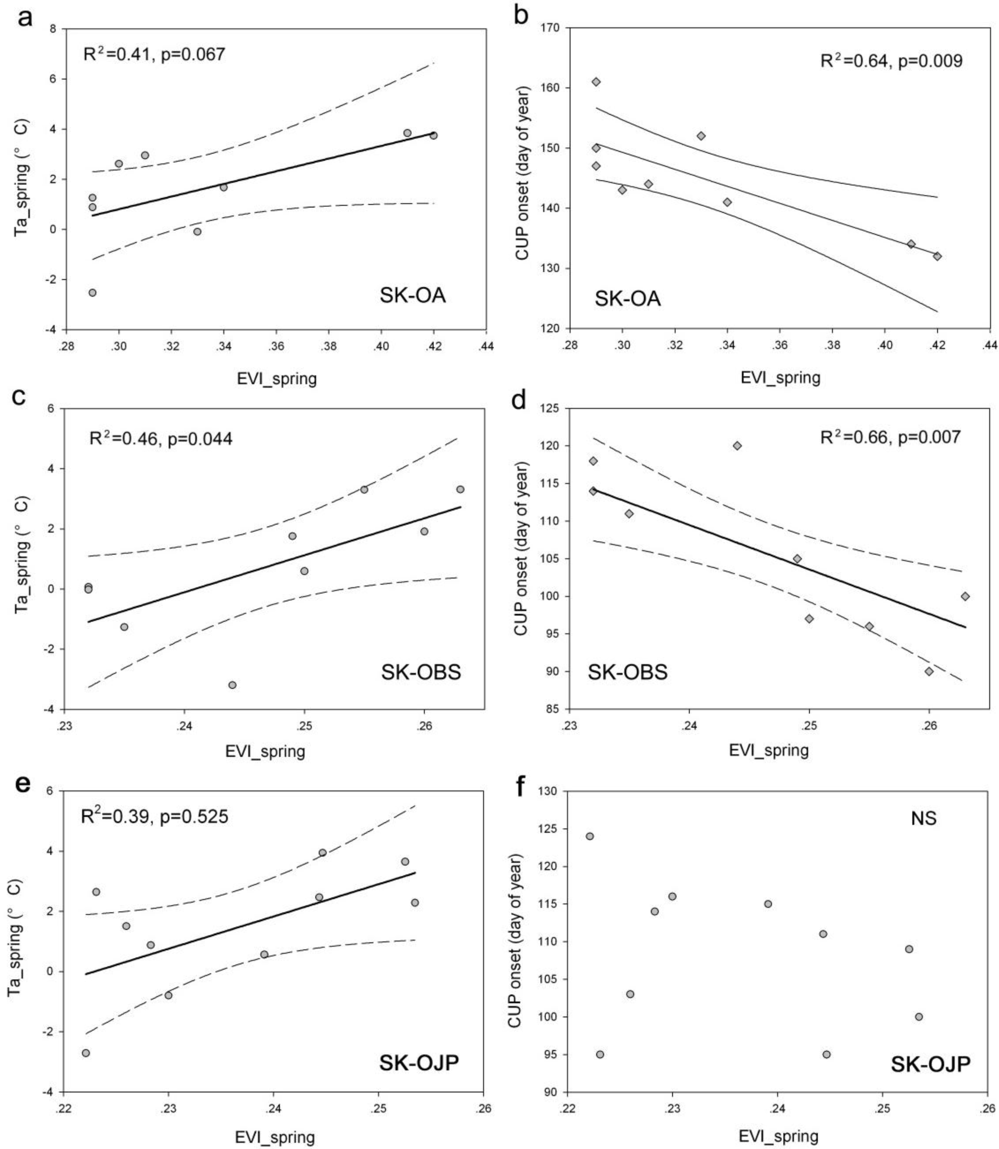
3.4. Relationships between Spring Temperature and C Fluxes

Spring temperature showed limited potential as a proxy for C fluxes at the SK-OA site, and no correlation was found between spring temperature and either annual GPP or NEP (Figure 5a,b). However, spring temperature was positively correlated with both GPP (R² = 0.47, p = 0.041 and R² = 0.63, p = 0.006) and NEP (R² = 0.49, p = 0.036 and R² = 0.40, p = 0.048) at the two evergreen sites.

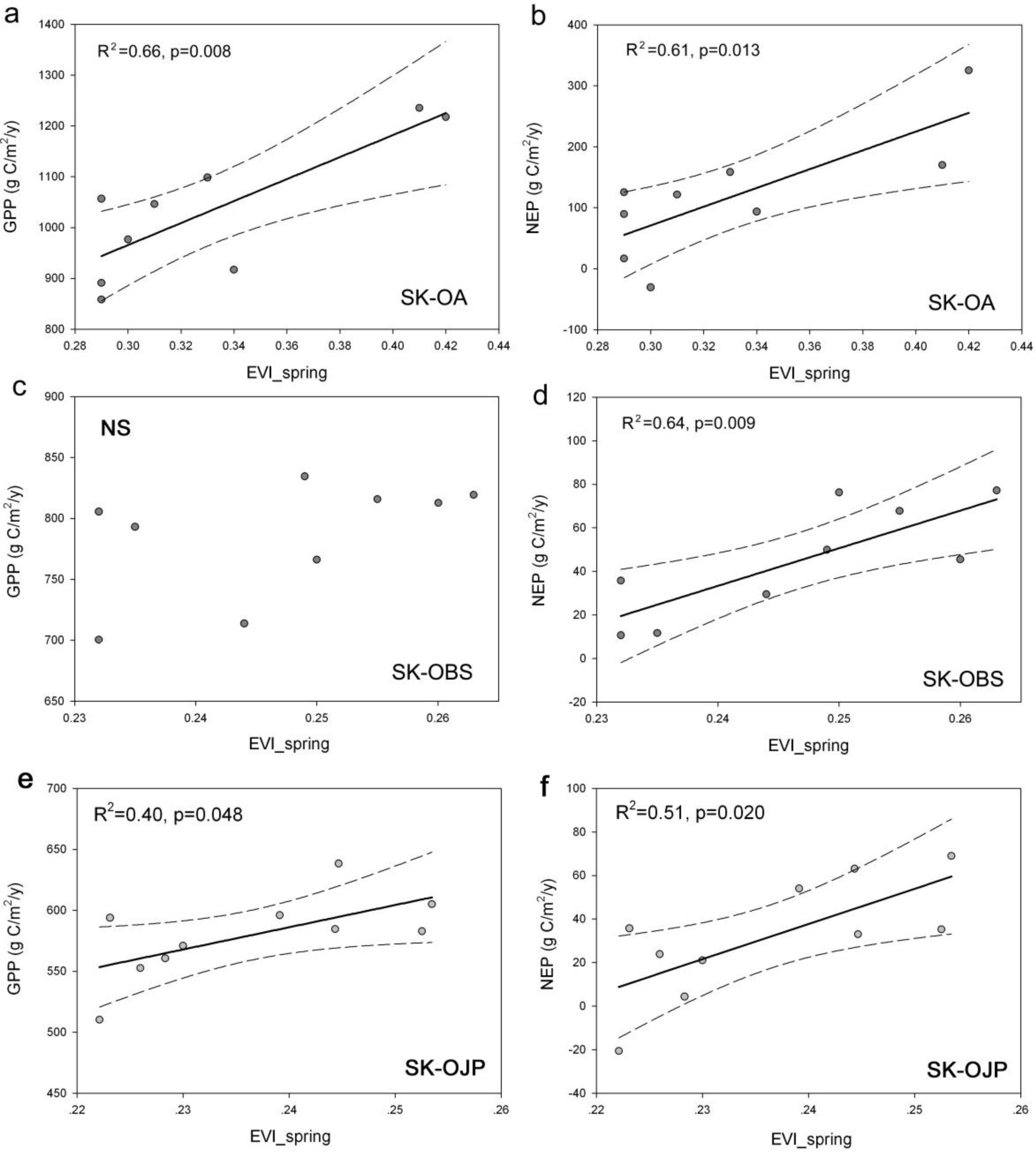
3.5. Relationships between Spring EVI and C Fluxes

Spring EVI was demonstrated to have a relatively consistent positive impact on C flux for all sites, although the level differed among the sites (Figure 6). High R² values of 0.66 (p = 0.008) and 0.61 (p = 0.013) were observed for spring EVI and GPP, and NEP for the SK-OA site. However, no significant correlation (R² = 0.26, p = 0.168) was found between spring EVI and GPP for the SK-OBS site. For SK-OJP, spring EVI was consistently correlated with annual GPP and NEP, with R² values of 0.40 (p = 0.048) and 0.51 (p = 0.020), respectively. At the deciduous site, SK-OA, spring EVI is a direct measure of canopy greenness and thus showed close relationships with both GPP and NEP. In contrast, SK-OBS showed limited variation in canopy greenness, and thus GPP showed low sensitivity to spring EVI changes. Interestingly, the NEP of the two evergreen sites showed high correlation with spring EVI. Although the GPP of SK-OBS was independent of spring EVI, our results suggest that spring variation in canopy greenness may have potential as an indicator of the annual NEP of both evergreen and deciduous sites in boreal regions. This would be of great significance for the remote evaluation of C sequestration among plant functional types, given the convenient acquisition of global EVI data from satellite observations.

4. Discussion

4.1. Comparison of the Spring Phenological Indicators

Among the spring phenological indicators, CUP onset is the best indicator of annual GPP, given its consistent and high correlation at all sites. These observations confirm that phenological indicators derived from the C flux data are possible indicators of C fluxes [1,4,8,9]. Our results further suggest that this correlation is independent of plant functional type, and so has considerable potential for future applications. However, three limitations constrain the application of CUP onset as a GPP proxy. First, this metric requires the measurement of NEE, which is limited by the number, distribution, and footprint of flux towers. Therefore, an upscaling algorithm is required to interpret the results of flux towers at a regional scale. Second, CUP onset is not appropriate for recently disturbed (i.e., fire, harvest) ecosystems that have only few days with a positive NEP over the whole year. This could be the major limitation to the use of CUP onset, considering the large areas of disturbed forest worldwide. The final uncertainty is that previous analyses have determined that CUP onset is a good indicator of annual NEP, which was not supported at the SK-OA and SK-OJP sites in our evaluation. A possible explanation is that in addition to spring phenology, summer drought may also influence the annual NEP for boreal forests, particularly for deciduous forest [35].

Spring temperature is a potential indicator of C fluxes for evergreen sites. However, its feasibility for deciduous sites is uncertain, and requires further in-depth evaluations. We used the air temperature recorded at the flux towers to calculate spring temperature; however, this method is limited by the availability of flux towers or weather stations. While remote-sensing technology can provide systemic observations of land surface temperature, the precision of these data is dependent on various factors [36]. These limitations likely restrict the use of spring temperature in operational applications.

We suggest that spring EVI would be better applied in future ecosystem models to enhance the simulation of the impact of climate change on C sequestration. Our results showed consistently high correlations between spring EVI and annual NEP for all sites. The most convenient aspect of EVI is that it can be acquired from time series data from satellite sensors, including MODIS and Landsat/TM [37]. In particular, assessing the feasibility of predicting a long-term EVI curve would greatly improve the data quality and facilitate ecosystem modeling [25,38]. Several studies have suggested the usefulness of satellite-based tools for phenology monitoring. This is supported by the strong correlation between spring EVI and the C flux phenology in our results, which is more appropriate for indicating net C exchange between the ecosystem and atmosphere [4,18,39]. One caveat for the application of remote-sensing data, however, is that they require the careful removal of uncertainties due to low solar illumination, the presence of ice/snow, and cloud cover in the high latitudes during the winter and early spring.

4.2. Impact of Plant Functional Type

We found that the deciduous site showed greater sensitivity to changes in spring phenology, as indicted by the greater slopes of the regressions (Figures 4 and 6). This is consistent with the observations of Euskirchen et al. [40] that deciduous species begin photosynthesis following leaf-out, and are characterized by a short and concentrated growing season. Therefore, GPP will have greater sensitivity to variation in the length of the growing season, as indicated by the CUP onset in our analysis. In contrast, the evergreen species exhibited low rates of photosynthesis for longer periods during the growing season, which leads in turn to low sensitivity in terms of the response of C flux to CUP onset.

In terms of plant functional type, spring temperature was a more appropriate indictor of C fluxes in the evergreen forest sites than for the deciduous forest site. Both GPP and NEP of deciduous ecosystems are related to phenology, which can be defined as the rhythm of growth. In contrast, the evergreen species may not show a clear pattern of canopy greenness during the growing season. Spring temperature could have played a greater role in controlling the growing rhythm than other environmental factors (e.g., water and radiation) for the evergreen species. Therefore, C fluxes of evergreen ecosystems are controlled more directly by temperature. These suggestions are supported by the more adaptive responses of evergreen ecosystems to environmental factors other than high-temperature-induced drought [41], and are consistent with the relative importance of environmental factors in several plant functional types [32].

5. Conclusions

Using flux measurements and time-series MODIS EVI products at three boreal forests in Canada, we analyzed and compared the potential of three spring phenological indicators of annual C fluxes. The C flux phenology, CUP onset, was an indicator of annual GPP at all sites, but was significantly correlated with annual NEP only at the SK-OBS site. Spring temperature showed limited potential as a proxy for C flux at the deciduous site, but represented a consistent measure of annual GPP and NEP at the two evergreen sites. While MODIS-derived spring EVI showed a weak correlation with GPP at the SK-OBS site, it exhibited a strong relationship with annual NEP at all sites, irrespective of differences in plant functional type. This finding is especially important as it provides a good proxy for net C uptake across species, and so will facilitate scaling up for regional and global analysis of the effects of climate change on C balance.

A potential limitation of our analysis is that we focused primarily on spring phenology, and autumn phenology might also have important effects on the annual C balance. This is in accordance with recent reports that autumn phenology regulates interannual NEP variability [1,5]. A combination of both would increase the power of ecosystem models to predict changes in C sequestration with future climate change. NEP also depends on stand age (i.e., different amplitudes in R_e), and given the mature and old forest sites examined in this study, our findings may not be applicable to young forests and other ecosystems (e.g., crops, grasslands). Because the components of soil respiration differ among forests of various ages [42,43], caution should be used when applying our results to young forests. Therefore, further analysis and evaluation would facilitate extension of our results to more ecosystems in diverse ecoregions.

References

1. Richardson, A.D.; Black, T.A.; Ciais, P.; Delbart, N.; Friedl, M.A.; Gobron, N.; Hollinger, D.Y.; Kutsch, W.L.; Longdoz, B.; Luyssaert, S.; et al. Influence of spring and autumn phenological transitions on forest ecosystem productivity. Philos. Trans. R. Soc. B-Biol. Sci 2010, 365, 3227–3246. [Google Scholar] [Green Version]
2. Wu, C.; Chen, J.M.; Gonsamo, A.; Price, D.T.; Black, T.A.; Kurz, W.A. Interannual variability of carbon sequestration is determined by the lag between ends of net uptake and photosynthesis: Evidence from long records of two contrasting forest stands. Agric. For. Meteorol 2012, 164, 29–38. [Google Scholar]
3. Gonsamo, A.; Chen, J.; Wu, C.; Dragoni, D. Predicting deciduous forest carbon uptake phenology by upscaling FLUXNET measurements using remote sensing data. Agric. For. Meteorol 2012, 165, 127–135. [Google Scholar]
4. Garrity, S.R.; Maurer, K.D.; Mueller, K.L.; Vogel, C.S.; Curtis, P.S. A comparison of multiple phenology data sources for estimating seasonal transitions in deciduous forest carbon exchange. Agric. For. Meteorol 2011, 151, 1741–1752. [Google Scholar]
5. Wu, C.; Chen, J.M.; Black, T.A.; Price, D.T.; Kurz, W.A.; Desai, A.R.; Gonsamo, A.; Jassal, R.S.; Gough, C.M.; Bohrer, G.; et al. Interannual variability of net ecosystem productivity in forests is explained by carbon flux phenology in autumn. Glob. Ecol. Biogeogr 2013, 22, 994–1006. [Google Scholar]
6. Xiao, J.; Zhuang, Q.; Baldocchi, D.D.; Law, B.E.; Richardson, A.D.; Chen, J.; Oren, R.; Starr, G.; Noormets, A.; Ma, S.; et al. Estimation of net ecosystem carbon exchange of the conterminous United States by combining MODIS and AmeriFlux data. Agric. For. Meteorol 2008, 148, 1827–1847. [Google Scholar]
7. Yuan, W.P.; Luo, Y.Q.; Richardson, A.D.; Oren, R.; Luyssaert, S.; Janssens, I.A.; Ceulemans, R.; Zhou, X.H.; Grunwald, T.; Aubinet, M.; et al. Latitudinal patterns of magnitude and interannual variability in net ecosystem exchange regulated by biological and environmental variables. Glob. Chang. Biol 2009, 15, 2905–2920. [Google Scholar]
8. White, M.A.; Running, S.W.; Thornton, P.E. The impact of growing-season length variability on carbon assimilation and evapotranspiration over 88 years in the eastern US deciduous forest. Int. J. Biometeorol 1998, 42, 139–145. [Google Scholar]
9. White, M.A.; Nemani, R.R. Canopy duration has little influence on annual carbon storage in the deciduous broad leaf forest. Glob. Chang. Biol 2003, 9, 967–972. [Google Scholar]
10. Wu, C.; Gonsamo, A.; Chen, J.M.; Kurz, W.A.; Price, D.T.; Lafleur, P.M.; Jassal, R.S.; Dragoni, D.; Bohrer, G.; Gough, C.M.; et al. Interannual and spatial impacts of phenological transitions, growing season length, and spring and autumn temperatures on carbon sequestration: A North America flux data synthesis. Glob. Planet. Chang 2012, 92, 179–190. [Google Scholar]
11. Thomas, C.K.; Law, B.E.; Irvine, J.; Martin, J.G.; Pettijohn, J.C.; Davis, K.J. Seasonal hydrology explains interannual and seasonal variation in carbon and water exchange in a semiarid mature ponderosa pine forest in central Oregon. J. Geophys. Res 2009, 114. [Google Scholar] [CrossRef]
12. Medvigy, D.; Wofsy, S.C.; Munger, J.W.; Hollinger, D.Y.; Moorcroft, P.R. Mechanistic scaling of ecosystem function and dynamics in space and time: The ecosystem demography model version 2. J. Geophys. Res 2009, 114. [Google Scholar] [CrossRef]
13. Chen, J.; Chen, W.; Liu, J.; Cihlar, J.; Gray, S. Annual carbon balance of Canada’s forests during 1895–1996. Glob. Biogeochem. Cy 2000, 14, 839–849. [Google Scholar]
14. Black, T.A.; Chen, W.J.; Barr, A.G.; Arain, M.A.; Chen, Z.; Nesic, Z.; Hogg, E.H.; Neumann, H.H.; Yang, P.C. Increased carbon sequestration by a boreal deciduous forest in years with a warm spring. Geophys. Res. Lett 2000, 27, 1271–1274. [Google Scholar]
15. Morgenstern, K.; Black, T.A.; Humphreys, E.R.; Griffis, T.J.; Drewitt, G.B.; Cai, T.; Nesic, Z.; Spittlehouse, D.L.; Livingston, N.J. Sensitivity and uncertainty of the carbon balance of a Pacific Northwest Douglas-fir forest during an El Nino LaNina cycle. Agric. For. Meteorol 2004, 123, 201–219. [Google Scholar]
16. Piao, S.; Ciais, P.; Friedlingstein, P.; Peylin, P.; Reichstein, M.; Luyssaert, S.; Margolis, H.; Fang, J.; Barr, A.; Chen, A.; et al. Net carbon dioxide losses of northern ecosystems in response to autumn warming. Nature 2008, 451, 49–52. [Google Scholar]
17. Baldocchi, D.B. Assessing the eddy covariance technique for evaluating carbon dioxide exchange rates of ecosystems: Past, present and future. Glob. Chang. Biol 2003, 9, 479–492. [Google Scholar]
18. Churkina, G.; Schimel, D.; Braswell, B.; Xiao, X. Spatial analysis of growing season length control over net ecosystem exchange. Glob. Chang. Biol 2005, 11, 1777–1787. [Google Scholar]
19. Piao, S.; Friedlingstein, P.; Ciais, P.; Viovy, N.; Demarty, J. Growing season extension and its impact on terrestrial carbon cycle in the Northern Hemisphere over the past 2 decades. Glob. Biogeochem. Cy 2007, 21. [Google Scholar] [CrossRef]
20. Zhang, X.; Friedl, M.A.; Schaaf, C.B.; Strahler, A.H.; Hodges, J.C.F.; Gao, F.; Reed, B.C.; Huete, A. Monitoring vegetation phenology using MODIS. Remote Sens. Environ 2003, 84, 471–475. [Google Scholar]
21. Liang, L.; Schwartz, M.D.; Fei, S. Validating satellite phenology through intensive ground observation and landscape scaling in a mixed seasonal forest. Remote Sens. Environ 2011, 115, 143–157. [Google Scholar]
22. Nagai, S.; Nasahara, K.N.; Muraoka, H.; Akiyama, T.; Tsuchida, S. Field experiments to test the use of the normalized-difference vegetation index for phenology detection. Agric. For. Meteorol 2010, 150, 152–160. [Google Scholar] [Green Version]
23. Dash, J.; Jeganathan, C.; Atkinson, P.M. The use of MERIS terrestrial chlorophyll index to study spatio-temporal variation in vegetation phenology over India. Remote Sens. Environ 2010, 114, 1388–1402. [Google Scholar]
24. Fisher, J.I.; Mustard, J.F. Cross-scalar satellite phenology from ground, Landsat, and MODIS data. Remote Sens. Environ 2007, 109, 261–273. [Google Scholar]
25. Ganguly, S.; Friedl, M.A.; Tan, B.; Zhang, X.; Verma, M. Land surface phenology from MODIS: Characterization of the collection 5 global land cover dynamics product. Remote Sens. Environ 2010, 114, 1805–1816. [Google Scholar]
26. Barr, A.G.; Black, T.A.; Hogg, E.H.; Kljun, N.; Morgenstern, K.; Nesic, Z. Interannual variability in the leaf area index of a boreal aspen-hazelnut forest in relation to net ecosystem production. Agric. For. Meteorol 2004, 126, 237–255. [Google Scholar]
27. Barr, A.G.; Black, T.A.; Hogg, E.H.; Griffis, T.J.; Morgenstern, K.; Kljun, N.; Theede, A.; Nesic, Z. Climatic controls on the carbon and water balances of a boreal aspen forest, 1994–2003. Glob. Chang. Biol 2007, 13, 561–576. [Google Scholar]
28. Law, B.E.; Falge, E.; Gu, L.; Baldocchi, D.D.; Bakwin, P.; Berbigier, P.; Davis, K.; Dolman, A.J.; Falk, M.; Fuentes, J.D.; et al. Environmental controls over carbon dioxide and water vapor exchange of terrestrial vegetation. Agric. For. Meteorol 2002, 113, 97–120. [Google Scholar]
29. DAAC, MODIS Land Product Subsets. Available online: http://www.modis.ornl.gov/modis/index.cfm (accessed on 4 March 2014).
30. Huete, A.; Didan, K.; Miura, T.; Rodriguez, E.P.; Gao, X.; Ferreira, L.G. Overview of the radiometric and biophysical performance of the MODIS vegetation indices. Remote Sens. Environ 2002, 83, 195–213. [Google Scholar]
31. Sims, D.A.; Rahman, A.F.; Cordova, V.D.; El-Masri, B.Z.; Baldocchi, D.D.; Bolstad, P.V.; Flanagan, L.B.; Goldstein, A.H.; Hollinger, D.Y.; Misson, L.; et al. A new model of gross primary productivity for North American ecosystems based solely on the enhanced vegetation index and land surface temperature from MODIS. Remote Sens. Environ 2008, 112, 1633–1646. [Google Scholar]
32. Wu, C.; Chen, J.M.; Huang, N. Predicting gross primary production from the enhanced vegetation index and photosynthetically active radiation: Evaluation and calibration. Remote Sens. Environ 2011, 115, 3424–3435. [Google Scholar]
33. Chen, B.; Coops, N.C.; Fu, D.; Margolis, H.A.; Amiro, B.D.; Barr, A.G.; Black, T.A.; Arain, M.A.; Bourque, C.P.A.; Flanagan, L.B.; et al. Assessing eddy-covariance flux tower location bias across the Fluxnet-Canada research network based on remote sensing and footprint modeling. Agric. For. Meteorol 2011, 151, 87–100. [Google Scholar]
34. Wu, C.; Chen, J.M.; Desai, A.R.; Hollinger, D.Y.; Arain, M.A.; Margolis, H.A.; Gough, C.M.; Staebler, R.M. Remote sensing of canopy light use efficiency in temperate and boreal forests of North America using MODIS imagery. Remote Sens. Environ 2012, 118, 60–72. [Google Scholar]
35. Welp, L.R.; Randerson, J.T.; Liu, H.P. The sensitivity of carbon fluxes to spring warming and summer drought depends on plant functional type in boreal forest ecosystems. Agric. For. Meteorol 2007, 147, 172–185. [Google Scholar]
36. Wan, Z. New refinements and validation of the MODIS land-surface temperature/emissivity products. Remote Sens. Environ 2008, 112, 59–74. [Google Scholar]
37. Pouliot, D.; Latifovic, R.; Fernandes, R.; Olthof, I. Evaluation of compositing period and AVHRR and MERIS combination for improvement of spring phenology detection in deciduous forests. Remote Sens. Environ 2011, 115, 158–166. [Google Scholar]
38. Gurung, R.B.; Breidt, F.J.; Dutin, A.; Ogle, S.M. Predicting Enhanced Vegetation Index (EVI) curves for ecosystem modeling applications. Remote Sens. Environ 2009, 113, 2186–2193. [Google Scholar]
39. Wu, C.; Gough, C.M.; Gonsamo, A.; Chen, J.M. Evidence of autumn phenology control on annual net ecosystem productivity in two temperate deciduous forests. Ecol. Eng 2013, 60, 88–95. [Google Scholar]
40. Euskirchen, E.S.; McGuire, A.D.; Kicklighter, D.W.; Davidm, W.; Zhuang, Q.; Clein, J.S.; Dargaville, R.J.; Dye, D.G.; Kimball, J.S.; McDonald, K.C.; et al. Importance of recent shifts in soil thermal dynamics on growing season length, productivity, and carbon sequestration in terrestrial high-latitude ecosystems. Glob. Chang. Biol 2006, 12, 731–750. [Google Scholar]
41. Griffis, T.J.; Black, T.A.; Morgenstern, K.; Barr, A.G.; Nesic, Z.; Drewitt, G.B.; Gaumont-Guay, D.; McCaughey, J.H. Ecophysiological controls on the carbon balance of three southern boreal forests. Agric. For. Meteorol 2003, 117, 53–71. [Google Scholar]
42. Makkonen, K.; Helmisaari, H.S. Fine root biomass and production in Scots pine stands in relation to stand age. Tree Physiol 2001, 21, 193–198. [Google Scholar]
43. Saurette, D.D.; Chang, S.X.; Thomas, B.R. Autotrophic and heterotrophic respiration rates across a chronosequence of hybrid poplar plantations in northern Alberta. Can. J. Soil Sci 2008, 88, 261–272. [Google Scholar]
Figure 1. An example determination of the C-uptake period (CUP) onset using daily net ecosystem production (NEP) for SK-OA in 2009. CUP onset was designated as the first day on which a positive daily NEP of the smoothed curve was observed.
Remotesensing 06 01991f1
Figure 2. Annual patterns of ecosystem C fluxes at (a) SK-OA, (b) SK-OBS, and (c) SK-OJP; histogram and point represent gross primary production (GPP) and net ecosystem production (NEP), respectively.
Remotesensing 06 01991f2
Figure 3. Relationships between spring EVI and (a) spring temperature (Ta_spring) for SK-OA, (b) carbon-uptake period (CUP) onset for SK-OA, (c) spring temperature (Ta_spring) SK-OBS, (d) CUP onset for SK-OBS, (e) spring temperature (Ta_spring) SK-OJP, and (f) CUP onset for SK-OJP. NS indicates no significant correlation. The solid and dashed lines represent regression and its 95% confidence of mean prediction.
Remotesensing 06 01991f3
Figure 4. Relationships between the C-uptake period onset (CUP) and (a) GPP of SK-OA, (b) NEP of SK-OA, (c) GPP of SK-OBS, (d) NEP of SK-OBS, (e) GPP of SK-OJP, and (f) NEP of SK-OJP. NS indicates no significant correlation. The solid and dashed lines represent regression and its 95% confidence of mean prediction.
Remotesensing 06 01991f4
Figure 5. Relationships between spring temperature and (a) GPP of SK-OA, (b) NEP of SK-OA, (c) GPP of SK-OBS, (d) NEP of SK-OBS, (e) GPP of SK-OJP, and (f) NEP of SK-OJP. NS indicates no significant correlation. The solid and dashed lines represent regression and its 95% confidence of mean prediction.
Remotesensing 06 01991f5
Figure 6. Relationships among spring enhanced vegetation index (EVI) and (a) GPP of SK-OA, (b) NEP of SK-OA, (c) GPP of SK-OBS, (d) NEP of SK-OBS, (e) GPP of SK-OJP, and (f) NEP of SK-OJP. NS indicates no significant correlation. The solid and dashed lines represent regression and its 95% confidence of mean prediction.
Remotesensing 06 01991f6