An Automated Approach to Map the History of Forest Disturbance from Insect Mortality and Harvest with Landsat Time-Series Data

Abstract

Forests contain a majority of the aboveground carbon (C) found in ecosystems, and understanding biomass lost from disturbance is essential to improve our C-cycle knowledge. Our study region in the Wisconsin and Minnesota Laurentian Forest had a strong decline in Normalized Difference Vegetation Index (NDVI) from 1982 to 2007, observed with the National Ocean and Atmospheric Administration’s (NOAA) series of Advanced Very High Resolution Radiometer (AVHRR). To understand the potential role of disturbances in the terrestrial C-cycle, we developed an algorithm to map forest disturbances from either harvest or insect outbreak for Landsat time-series stacks. We merged two image analysis approaches into one algorithm to monitor forest change that included: (1) multiple disturbance index thresholds to capture clear-cut harvest; and (2) a spectral trajectory-based image analysis with multiple confidence interval thresholds to map insect outbreak. We produced 20 maps and evaluated classification accuracy with air-photos and insect air-survey data to understand the performance of our algorithm. We achieved overall accuracies ranging from 65% to 75%, with an average accuracy of 72%. The producer’s and user’s accuracy ranged from a maximum of 32% to 70% for insect disturbance, 60% to 76% for insect mortality and 82% to 88% for harvested forest, which was the dominant disturbance agent. Forest disturbances accounted for 22% of total forested area (7349 km²). Our algorithm provides a basic approach to map disturbance history where large impacts to forest stands have occurred and highlights the limited spectral sensitivity of Landsat time-series to outbreaks of defoliating insects. We found that only harvest and insect mortality events can be mapped with adequate accuracy with a non-annual Landsat time-series. This limited our land cover understanding of NDVI decline drivers. We demonstrate that to capture more subtle disturbances with spectral trajectories, future observations must be temporally dense to distinguish between type and frequency in heterogeneous landscapes.

1. Introduction

Understanding forest carbon (C) dynamics at the management scale is critical, because forests contain ∼90% of aboveground terrestrial C stocks [1]. Prior studies have found North American forests to be a large C sink that offsets global anthropogenic C emissions [2–4]. Due to changes in forest disturbance rates and other processes that can reduce forest productivity, the long-term strength of this C sink is uncertain [5]. Monitoring and understanding disturbance dynamics at the landscape scale that can alter forest C is important so that future management activities can optimize C sequestration [6,7].

In this study, we focused on the northern forests of Wisconsin and Minnesota (Laurentian Forest) that experienced a substantial decline in productivity from 1982 to 2007. This decline was observed at 8-km resolution by the Global Inventory Modeling and Mapping Studies (GIMMS) Normalized Difference Vegetation Index (NDVI) data version “g”, derived from the National Ocean and Atmospheric Administration’s (NOAA) series of Advanced Very High-Resolution Radiometers (AVHRRs) [8]. We assumed that NDVI was a surrogate for photosynthetic capacity and a measure of vegetation health or vitality [9]. NDVI is related to the structural properties of plants, including Leaf Area Index (LAI), Absorbed Photosynthetically Active Radiation (APAR) and leaf biomass [10]. Widespread AVHRR NDVI declines have been reported further north in the Canadian boreal forest and have been associated with disturbances from fire, insect outbreak and changes in climate [11–16]. However, these boreal forests have limited human access and have not had a decline in NDVI throughout the 1982 to 2007 AVHRR record of measurements.

Landsat is one of our best means to understand long-term land cover change and its impact on regional vegetation productivity. Many anthropogenic land cover changes occur at less than a 250-m resolution [17]. The Landsat series of instruments at a 30-m resolution provide a critical tool to understand forest changes relevant to the C-cycle from harvest [18], wildfire [19,20] and insect outbreaks [21] by extending observational studies to areas that have poor records [22]. North American studies have used the decadal epoch of Landsat data, GeoCover or the Global Land Survey (GLS) [23] to quantify forest disturbances [24,25], while others have used dense Landsat time-series stack (LTSS) data focused on specific regions to evaluate change vectors to understand forest disturbance dynamics [20,26–29]. These LTSS data with ecosystem models could be used to monitor the productivity of forests pre- and post-disturbance [30].

Due to the ease of extraction, many remote sensing studies using Landsat have focused on fire disturbance and logging [20,31–35]. Given the difficulty of discriminating background populations from outbreak events, few have classified insect, pest and pathogen events in Landsat data [21,36]. Widespread insect infestations have occurred in North America over the past 30+ years, which have potentially large impacts on standing C stocks [37,38]. Extracting disturbance information from satellite records with more advanced algorithms has already shown promise [21,39] and could help resolve disturbance processes for C-cycle models.

Many existing remote sensing studies of forest disturbance using Landsat time-series stacks (LTSS) lack causal information that is critical for C-cycle models to quantify C-cycle dynamics [18,27,29]. For example, an algorithm developed by Huang et al. 2010 [29] has been implemented wall-to-wall for the continental US and has been shown to be very effective at mapping clear cut harvest, but has also been noted to have difficulty in complex heterogeneous landscapes [40]. This algorithm uses the concept of normalized values for pixels based on the mean and standard deviation of known forest pixels from the same scene and uses multiple images to improve the forest/non-forest classification. Another algorithm, LandTrendr, by Kennedy et al. 2010 [27] uses an automated trajectory-based image analysis and allows users to automatically identify and segment different pixel trends in land cover change through time.

These algorithms do not attempt to define forest disturbance type, and this information is needed to account for different C-cycle processes. Clear cut harvest has a much different C-cycle pathway than insect-induced mortality. Harvest removes above ground biomass and transports it from the region to be used in building materials, pulp and paper, etc.; this results in a net C sink from biomass export; whereas insect-induced mortality would result in high levels of standing dead biomass that could decompose and respire to the atmosphere for many years into the future [1]. This difference in the C pathway can change a region from a net sink to a net source, and the disturbance type should be considered when attempting to model regional C-cycle dynamics. Considering the large extent and duration of the AVHRR NDVI decline, we sought to understand causal factors. The Laurentian Forest region provides a unique opportunity to test an algorithm that maps different disturbances through time. Developing and testing an algorithm’s performance on a Landsat time-series where historical disturbances have occurred could improve our understanding of C-cycle dynamics by providing the location, time, type and extent of disturbance. This information is critical to reduce our C-cycle model uncertainties.

To investigate declines in forest productivity and evaluate Landsat disturbance classification performance in the Laurentian Forest, we developed a series of questions. First, were the long-term declines in forest productivity an error or real? Second, can an image classification algorithm be used on Landsat time-series data to extract forest disturbances reliably for a region with heterogeneous canopy cover? Third, what dominant disturbance agent caused the NDVI decline at the coarse scale?

Here, we attempt to extract causal information by combining available in situ data with a semi-annual LTSS classification algorithm, and we evaluate the accuracy of our algorithm by dominant disturbance types within path/rows that have different rates and types of disturbance. Our objective was to develop a simple, efficient and effective tool to distinguish between clear cut harvests and insect disturbance in the Laurentian Forest. We sought to evaluate with ancillary data if using a LTSS algorithm can enhance our understanding of forest disturbance dynamics.

2. Data and Methods

We use two of the longest satellite records available to understand long-term declines in forest productivity. By coupling multi-resolution data, our intent was to understand scale differences in observations. We attempt to define the type of event and temporal nature of the trend from a few proven spectral indices with simple threshold and trajectory techniques [21,41]. Our classification approach relies on growing season time-series analysis to extract disturbed area through time in an attempt to understand declines in forest productivity. Our approach provides a systematic manner to distinguish between clear cut harvest and insect outbreak, while resolving why a multi-decade AVHRR NDVI decline can occur in a forested landscape.

2.1. Study Area

Our study region, the Laurentian Forest, is a mix of deciduous and evergreen stands with many lowland bogs and wetlands. Numerous disturbance events from insect outbreaks and salvage logging have been reported in this region over previous decades that could have possibly been observed at the 8-km NDVI pixel scale [42–44]. Reinikainen et al. 2012 [45] suggested that larger harvest patch sizes have increased the openness of the landscape in this region. This could have altered vegetation productivity observed by coarse-resolution AVHRR. Due to the complex nature of multiple land cover disturbance events reported by other studies [42–44], we have attempted to understand and quantify these dynamics at the Landsat 30-m scale on a semi-annual basis.

We used NDVI data derived from GIMMS version “g” [8], because a consistent inter-calibrated record is needed to calculate anomalies that contain changes in the photosynthetic capacity of vegetation. These data are maximum values composited [46] to 8 km by 8 km, have been processed to account for orbital drift, minimize cloud cover and compensate for sensor degradation and the effects of stratospheric volcanic aerosols [8,47,48]. NDVI was calculated from AVHRR Channel 1 (0.58–0.68 μm) and Channel 2 (0.72–1.10 μm) as:

$$\mathit{NDVI}=(\mathit{Channel} 2-\mathit{Channel} 1)/(\mathit{Channel} 2+\mathit{Channel} 1)$$

(1)

Our AVHRR anomaly map was calculated as the mean growing season (May to September) per-pixel value per-year with a least squares linear fit applied from 1982 to 2007. We selected the Laurentian Forest for further study, because it met two criteria: (1) it is a contiguous region greater than 2000 km² with a negative NDVI trend stronger than −0.05 at a 98% confidence interval from 1992 to 2005 in GIMMS 3g NDVI data and a 1982 to 2007 negative trend in GIMMS g NDVI data [24]; and (2) semi-annual LTSS, high-resolution aerial photo validation data and aerial field survey data of annual disturbances from 1996 through 2006 exist. Previous work by Slayback et al., 2003 [49], established that robust trends in AVHRR NDVI exist with significance levels greater than 90%. Neigh et al. 2008 [24] also found that robust changes in AVHRR NDVI at significance levels greater than 98% could be associated with forest disturbances. Figure 1 displays the distribution of 8-km GIMMS AVHRR NDVI g pixels with a negative trend stronger than −0.05 between 1982 and 2007 overlaid upon one date of Landsat images used in classifications. Additional independent disturbance data are overlaid, including annual aerial insect disturbance survey’s from 1996 to 2006, fire disturbance data from monitoring trends in burning severity (MTBS) from 1984 to 2007 [50] and aerial photo high resolution sites used for classification evaluation.

2.2. Landsat Data

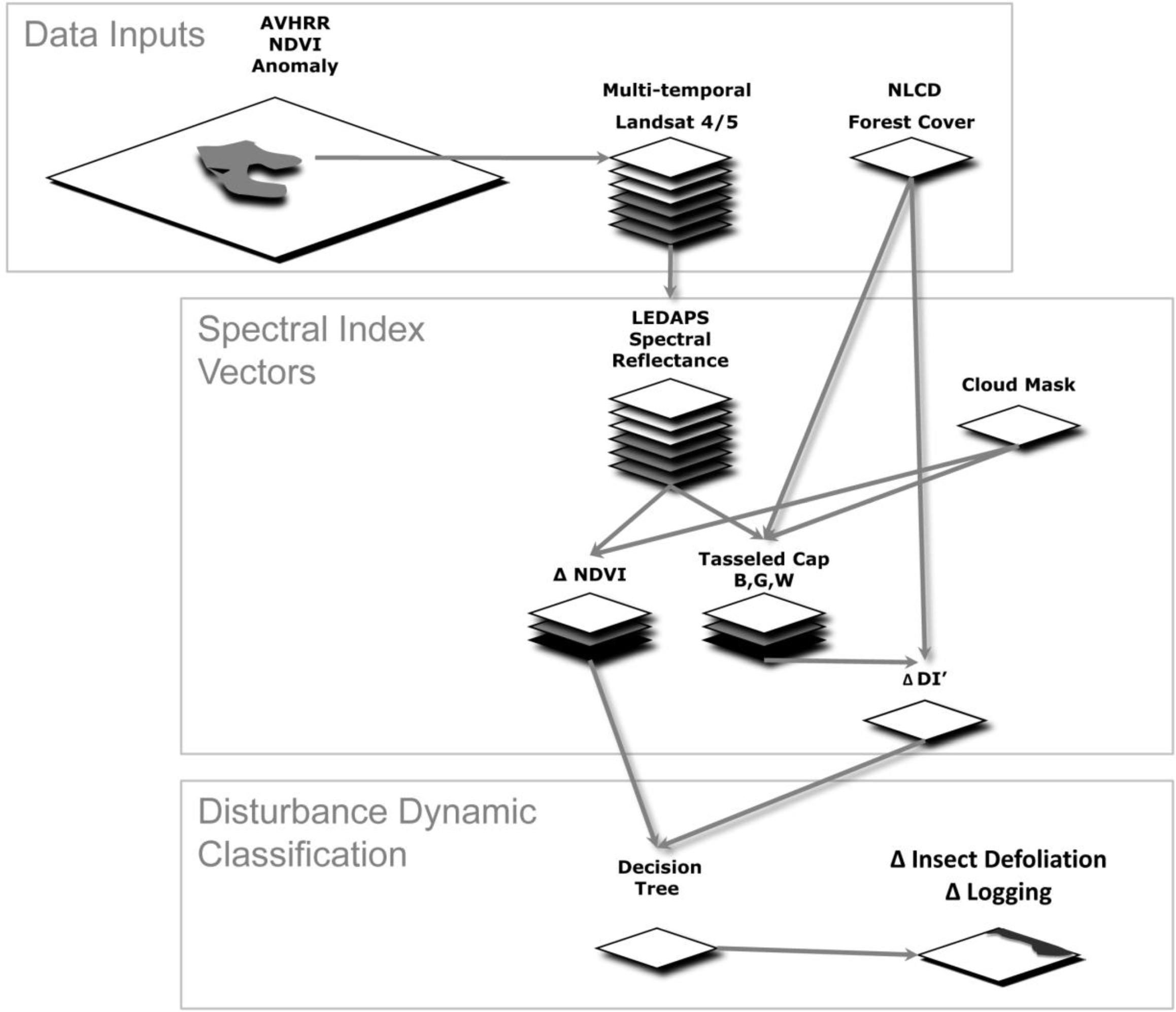
Landsat 5 data were acquired from the United States Geological Survey (USGS) global visualization viewer [51] for four path/rows covering the same extent as the AVHRR negative anomaly. We selected 11 to 13 images per path/row for analysis, all with less than 20% cloud cover, spanning from 1984 to 2006. We avoided using Landsat 7 ETM+ imagery, so that we would not need to contend with the scan line correction (SLC) problem. Our process could have used Landsat 7 data images if no data values are treated as a cloud mask from the outset. Each image followed a processing procedure with four primary parts. First, the Landsat Ecosystem Disturbance Adaptive Processing System (LEDAPS) time-series surface reflectance calculation was performed. Second, a cloud screen was applied, masking all pixels that could not be used for change detection. Third, spectral indices were generated by NDVI, Tasseled Cap and a Disturbance Index (DI’). The fourth and final step was disturbance dynamic characterization based on the index threshold, and the remaining pixels were subsequently processed by spectral trajectory.

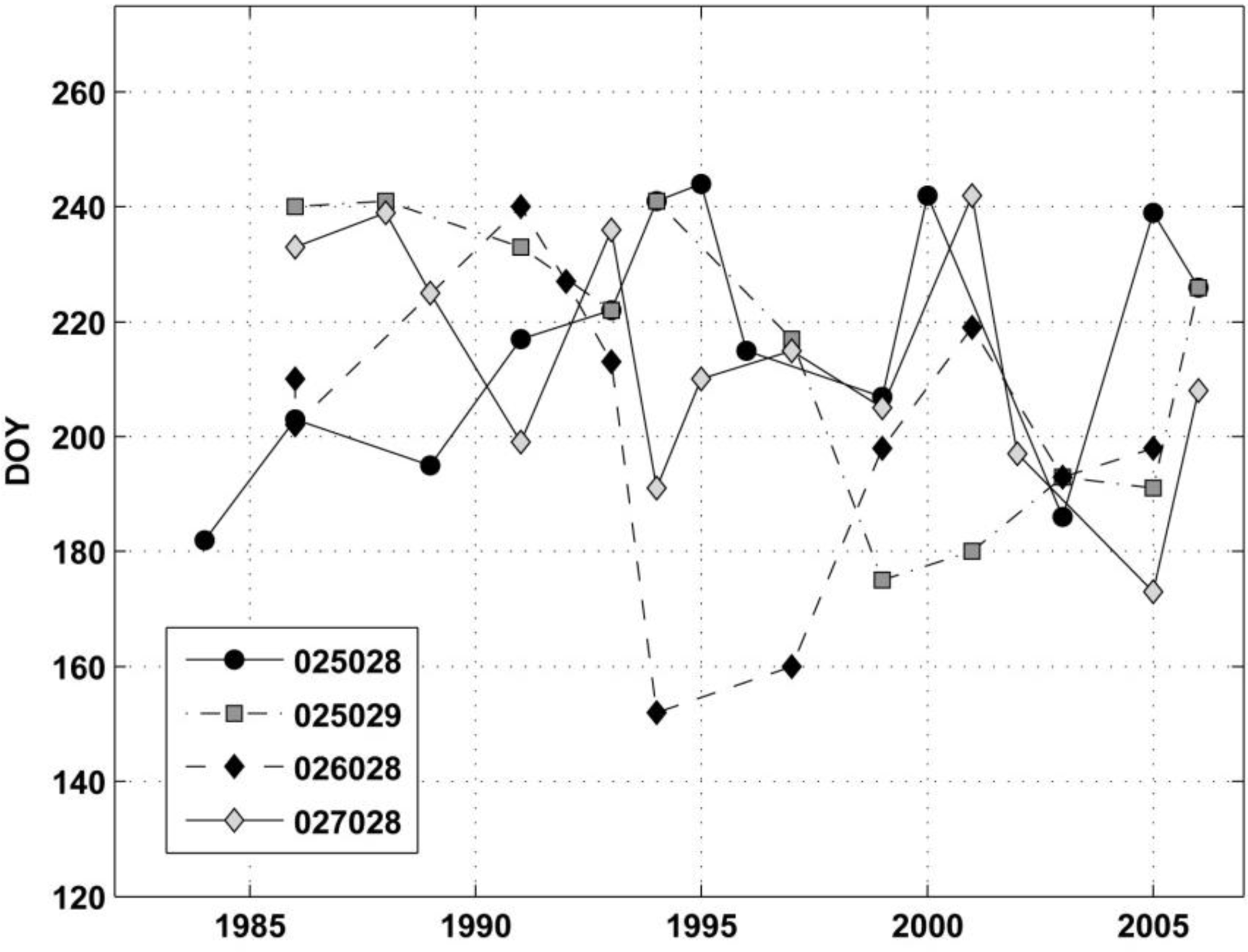
We provide a schematic of our approach in Figure 2, with the Landsat day of year (DOY) acquisition from our selected four path/rows within the AVHRR negative trend anomaly in Figure 3. A majority of the Landsat images we selected for analysis were peak growing season (Julian Days 175 to 245, late June through early September), with only two images in our analysis from early June. One disadvantage of tracking trends in disturbance for this region is the lack of dense Landsat growing season data. This potentially reduces our ability to capture disturbance events and trends.

Image processing included a number of steps to extract temporal indices that were relevant to our objectives. We used the LEDAPS algorithm for the calculation of surface reflectance to minimize the impacts of atmospheric, solar zenith angle and sensor degradation artifacts that can impair the quality of long-term analysis of spectral indices [25]. Cloud screening is critical to dense time-series analysis of Landsat, because abrupt changes in surface reflectance can obscure major land surface changes. All subsequent threshold values use surface reflectance scaled by multiplying times ten thousand.

We generated three primary spectral indices to evaluate the optical properties of logging and insect disturbance throughout the Laurentian Forest: NDVI, the Tasseled Cap of brightness, greenness and wetness and a disturbance index, which has been used to identify forest disturbances in other regions [39].

NDVI [9] from Landsat was calculated as:

$$\mathit{Landsat} \mathit{NDVI}=((\mathit{Channel} 4-\mathit{Channel} 3)/(\mathit{Channel} 4+\mathit{Channel} 3))$$

(2)

The Tasseled Cap used coefficients from Crist and Cicone, 1984 [52], which were implemented for Landsat 5 surface reflectance data. Transforming images to Tasseled Cap space aided in image normalization, because weighted components are sensor specific and not scene dependent [53]. In our analysis, the third component “wetness” is considered a measure of the soil moisture content of the target and is orthogonal to “brightness” and “greenness”, which is a similar approach to principle component analysis. We use these orthogonal components to discriminate specific properties of targets. The disturbance index (DI’) is based upon the concept that a different spectral response of a stand replacing disturbance will occur with a higher reflectance of brightness and a lower reflectance of greenness and wetness [54].

We calculated DI’ as follows:

$$D{I}^{\prime }=\mathit{Wetness}-\mathit{Brightness}$$

(3)

It has been noted by Hais et al., 2008 [39], that forest stands impacted by pine beetle are better detected using indices that enhance the SWIR “wetness” and that using DI’ can enhance the spectral response of insect forest disturbances. Forest stands impacted by pine beetle have been detected using indices that employ reflectance information from the 1.55–1.75 μm and 2.1–2.3μm Landsat Thematic Mapper bands, and using a normalized disturbance index can better differentiate insect forest disturbances from logging [39].

2.2.1. Landsat Forest Mask

We delineated forest from agriculture through simple threshold values through the image stack on brightness, NDVI and the National Land Cover Database [55], applying a similar approach as Vieira et al., 2003 [56]. The mean brightness of the image time-series in forested National Land Cover Database (NLCD) pixels was used as a threshold to remove young bright stands of forest less than three years old and agriculture, which typically has a higher soil reflectance. We applied an NDVI threshold of less than 0.45 to remove sparsely vegetated areas in the 2001 NLCD forested classes. We applied these thresholds, because the NLCD does not account for changes in forest cover. In addition, we used agriculture and wetland classes from NLCD to exclude these areas from our analysis.

2.2.2. Landsat Cloud Masking

We employed an automated cloud and cloud-shadow detection method for Landsat data that largely avoided post-classification manual corrections for cloud and cloud-shadow artifacts. We build upon concepts developed in the prior automatic cloud cover assessment (ACCA) algorithm [57] to improve the discrimination of cloud and shadow on a per-pixel basis [58]. Instead of relying on information from a single date of imagery, clouds were identified as deviations from the mean Tasseled Cap brightness and thermal band values through time for each Landsat pixel. Pixels where the brightness value was more than two standard deviations above the long-term mean and the temperature more than one standard deviation below were identified as cloud tops. The solar zenith angle was then used to determine the direction to the cloud shadow. Pixels in the direction of the cloud shadow that experienced a drop in brightness of more than one standard deviation relative to the long-term mean were identified as cloud shadow. As the distance to shadow can vary as a function of cloud height and cloud height is inherently related to the temperature of the cloud, a simple relationship between minimum cloud temperature and distance to shadow was developed to limit the number of pixels that were searched for cloud shadows. A final filter was applied to each 3 × 3 moving pixel window, where the center pixel would only be classified as cloud or cloud shadow if more than half of the nine pixels in the sample window were also classified as cloud or shadow to reduce spurious per-pixel errors. We also buffered defined cloud and shadow with a 5 × 5 moving pixel window to account for edge artifacts.

2.2.3. Landsat Disturbance Classification

Hierarchical thresholds of our decision tree at each junction in the classification were defined with the following equations.

$$\mathrm{\Delta }D{I}^{\prime }=D{I^{\prime }}_{y+1}-D{I^{\prime }}_y$$

(4)

where ΔDI' is equal to a change in normalized disturbance subtracted from one year (DI'_y) to the next available image in the stack (DI'_{y + 1}) on a per-pixel basis.

$$\mathrm{\Delta }\mathit{Ld}=\mathrm{\Delta }D{I}^{\prime }>L_{\mathit{th}}$$

(5)

where logging disturbance (ΔLd) is equal to a change in the normalized disturbance index (ΔDI') greater than an adjusted range of logging DI’ threshold values (L_th). The range of L_th values to produce multiple maps was determined from a subset of the image stack and a subset of the air-photo training data. The date of disturbance is labeled as the date post decline from one year to the next in the Landsat stack.

We defined insect disturbance with a trajectory approach applying the following equation:

$$\mathrm{\Delta }\mathit{Id}=\left(\mathrm{\Delta }D{I^{\prime }}_{5\hspace{0.17em}\mathit{yrs}}<-750\right)*\left({\mathit{Slope}}_{5\hspace{0.17em}\mathit{yrs}}<-150\right)*\left(p_{5\hspace{0.17em}\mathit{yrs}}<p_{\mathit{th}}\right)$$

(6)

where (ΔId) is a change in insect disturbance for a five-year time span. First, to reduce computation time, the change in DI' over a five year time span (ΔDI'_{5 yrs}) was defined as <−750. A linear regression was then fit to each pixel meeting this criterion. Pixels were classified as insect disturbed if the slope over this five-year period (Slope_{5 yrs}) was less than −150 with a significance (p_{5 yrs}) below an ensemble threshold (p_th) ranging from 0.01, 0.05, 0.1 and 0.15 increments. The date of disturbance is labeled as the last year in the decline sequence. Note that a limitation exists with this method, as pixels with less than 3 values per 5 year interval are not computed. These pixels could be contaminated by clouds or cloud shadow. This method was applied incrementally for each Landsat stack (i.e., 1984 to 1988, 1985 to 1989, 2002 to 2006). We established the change in slope values by using ancillary insect air-survey data as training.

Without a salvage logging class, many cleared sites were defined initially as insect outbreak. To capture salvage logging, we applied the following equation to pixels classified as insect outbreak:

$$\mathrm{\Delta }\mathit{Ldslvg}=\left(\sum \mathit{tn} D{I}^{\prime }<\frac{L_{\mathit{th}}}{2}\right)<p_{\mathit{th}}$$

(7)

where the salvage logged (ΔLdslvg) has a decline half as great as the prescribed logging threshold. All salvage logging classed pixels were later reclassified as logged for classification evaluation purposes. Our approach is simple and straight forward and enables many LTSSs to be processed on a standard desktop workstation. The splits in the decision tree first rely on a per-pixel change in a prescribed threshold value; if no change is detected, then the spectral trajectory approach is applied.

2.2.4. Running Landsat Classifications

We ran our classification with multiple decision tree splits producing 20 iterations by varying thresholds of ΔDI’ (−9000 = moderate intensity to −5000 = low intensity, with increments of 1000) for observed spectral logging signatures, and p (0.01, 0.05, 0.1 and 0.15) for systematic forest insect decline. This process alters tree splits of change and no-change and potentially alters mapping accuracy. Our basic assumption with this algorithm is that clear cut harvest will have a rapid change in DI’ from one image to the next, and insect disturbance will have a more gradual spectral change.

We then compared all 20 maps to our high-resolution (<2 m) air-photo dataset to provide an optimized accuracy assessment. This produced 80 classifications (20 iterations times four Landsat stacks) for error assessment with all classification ensembles sieved to 90 m to reduce speckle in classified outputs. We believe this approach justified decision tree splits statistically with validation data as opposed to introducing analyst biases and provided information about the sensitivity of the algorithm to clear cuts and insect outbreak. This approach represents a substantial difference in prior methods, as it provides error bounds or uncertainty of classification accuracy not discussed in other forest disturbance mapping assessments.

2.2.5. Independent Classification Evaluation Data

LTSS studies are often restricted in their ability to have a comprehensive independent evaluation dataset, and past studies have used the Landsat data itself with analyst interpretation to validate their classification [25,29,59]. This limitation is imposed, because of the lack of a dense annual time-series in other remote sensing products. To alleviate this, we used a combination of historical aerial interpreted photographs with disturbance maps from land management agencies. Change or disturbance-based classifications require time-series reference data to define change areas through auto segmentation, or they are manually digitized by experienced image analysts [25,29,60]. We collected aerial photography from the National Historical Air Photo Archive (NHAP) for the early 1980s and the National Agriculture Imagery Program (NAIP) for the early 1990s and 2000s to evaluate the forest harvest and insect disturbances that we detected with our classification. A subset of one NHAP/NAIP image stack was used for training to establish a range of thresholds. We provide dates and image center coordinates in

Table 1. Five locations of air photo stack classification evaluation data listed sequentially by Landsat WRS 2 path/row and the collection date of the photo stack bounds that are displayed in yellow in Figure 1.

Center DD+					Spatial	Spec.
Path Row	Lat	Lon	Air Photo ID	Date	Res.	Res.	Ortho	Source
025028	45.9033	−91.0890	NC1NHAP810479086	06/06/88	2 m	CIR	Y	GloVis *
			N10NAPPW05469064	05/07/92	1 m	B/W Pan	Y	GloVis *
			N10NAPPW10405076	04/22/98	1 m	B/W Pan	Y	GloVis *
			Sawyer County, WI	09/16/04	1 m	True Color	Y	wisc-view t
			Sawyer County, WI	08/03/06	1 m	True Color	Y	wisc-view t
025029	43.9375	−90.0622	NC1NHAP800299096	10/28/80	2 m	CIR	Y	GloVis *
			NC1NHAP020337057	06/03/86	2 m	CIR	Y	GloVis *
			N10NAPPW05439155	05/06/92	1 m	B/W Pan	Y	GloVis *
			N10NAPPW10423007	04/27/98	1 m	B/W Pan	Y	GloVis *
			Juneau County, WI	09/01/05	1 m	True Color	Y	wisc-view t
			Juneau County, WI	06/01/06	1 m	True Color	Y	wisc-view t
			Juneau County, WI	09/20/08	1 m	True Color	Y	wisc-view t
026028	46.2083	−91.5217	NC1NHAP020435130	06/06/88	2 m	CIR	Y	GloVis *
			N10NAPPW05487025	05/05/92	2 m	B/W Pan	Y	GloVis *
			N10NAPPW10407136	04/22/98	2 m	B/W Pan	Y	GloVis *
	43.9670	−90.0584	NC1NHAP020435130	06/06/88	2 m	CIR	Y	GloVis *
			N10NAPPW02691570	05/05/92	2 m	B/W Pan	Y	GloVis *
			Bayfield, WI	09/01/05	1 m	True Color	Y	wisc-view t
027028	46.4165	−93.1877	NC1NHAP840067163	04/17/84	2 m	CIR	Y	GloVis *
			NP0NAPP003135084	04/21/91	2 m	B/W Pan	Y	GloVis *
			N1NAPPW08876068	06/01/97	2 m	B/W Pan	Y	GloVis *
			Aitkin County, MN	09/01/03	1 m	True Color	Y	wisc-view t

⁺Center latitude and longitude calculated from earliest air photo corner bounding coordinates in decimal degrees;

^*United States Geological Survey (USGS) global visualization server (GloVis) [51]. We orthorectified air photos using the PCI Geomatica OrthoEngine using camera model information;

^tWisconsinView [62] corrected National Agriculture Imagery Program (NAIP) data for terrain and camera angle displacement; accuracy: ± 5 m when compared to mosaicked digital orthophoto quadrangle; the imagery is a subset from a histogram-balanced mosaic.

. Raw data were orthorectified using Geomatica’s OrthoEngine, with camera calibration information derived from the USGS to remove terrain spatial error artifacts that could be introduced in automated per-pixel validation cross comparisons [61]. Five sites were selected with air-photo stacks ranging from 4 to 7 images per site; air-photos were less than 2-m in resolution and were panchromatic and false color near-infrared. Air-photo stack sites were constrained by the availability of growing season multiple overlapping photos available in archives. Early and late images were used to evaluate forest/non-forest (logged conditions). The Landsat disturbance classification was evaluated with high-resolution air-photos, and if a partial disturbance was found within a Landsat pixel, it was considered disturbed. If mixed disturbance agents existed within a Landsat pixel, the analyst selected the dominant agent.

2.2.6. Ancillary Data

Additional datasets were also used when assessing time-series-related classification products. Monitoring trends in burn severity data [62] were used as an independent source to confirm negligible fire activity in the study region. Monitoring trends in burn severity is a multi-year project designed to map burn severity perimeters at 30 × 30 m for fires larger than 1000 acres across the United States from 1984 through 2010. These data are based upon Landsat Thematic Mapper data and use the normalized burn ratio. The normalized burn ratio index has been found to be a useful indicator to define the spatial distribution of burn severity and has been actively used in a number of long-term studies [63,64].

Due to the limited time record of aerial photography and potentially subtle multi-year insect disturbance, we used the Wisconsin and Minnesota insect disturbance database. These data were produced by the Forest Health Protection, United States Department of Agriculture (USDA) Forest Service [65], which has mapped annual insect outbreaks from 1996 to 2006 for our study region. These data are derived from aerial surveys in which interpreters hand-delineate outbreak areas in conjunction with site visits on the ground to confirm accuracy. The primary disadvantage of these data is that they are subjective, with accuracy depending upon the competence of the sketch mapper and the conditions under which the data were obtained [66,67]. These uncertainties limit the ability of these data to be useful in per-pixel assessment of insect disturbance. The assumption that the reference image used in photo-interpretation is 100% correct is rarely valid [68–70]. We evaluated the ability of LTSS data to capture these disturbances. We also collected forest species data from the USDA Forest Service Forest Inventory and Analysis (FIA) program to understand which cover-types experienced a decline in productivity.

Our intent was to identify substantial forest ecosystem C-cycle disturbance events with Landsat time-series data and relate these events to trends in NDVI at the 8-km scale. Acquiring ancillary data provided the means to understand major disturbance events that Landsat may not be able to detect. We had no intent to classify specific insect outbreak types with Landsat, and this falls beyond the scope of this study. We also acknowledge the limitations of our Landsat stacks to detect defoliation events.

2.2.7. Landsat Classification Evaluation Procedure

We applied three main considerations when developing our classification evaluation sampling strategy, which included: (1) sampling units; (2) design; and (3) sampling size [71,72]. When considering the sampling unit for classification evaluation, a subset area within an image is often preferred. We applied two-stage cluster sampling, the original sample area of the air-photo and a sub-sampling of the original subset area within the air-photo. This is undertaken to reduce the amount of reference data required [72]. Congalton, 1988 [73], suggested limiting the cluster sample size from 10 to 25 pixels to reduce redundancy and over representation of a single class. Sampling units for image classification are typically clusters of pixels used as a single sample (e.g., a 3 × 3 pixel block) to reduce the effect of registration errors between the reference data and map locations [74–77]. We applied this approach to ensure adequate representation of air-photo evaluation data compared to classified classes.

Random stratified sampling has been identified as the most precise and appropriate strategy for image classifications that contain rare classes, such as change or disturbance, as it ensures that all classes are represented [29,76,78]. Random sample selection provides satisfactory and often the most accurate assessment of land cover change classification accuracy [75,78]. Congalton, 2004 [79], suggested sample sizes of more than 50 for each class or, as suggested by Chen and Wei, 2009 [74], 75 to 100 for a large study area or a large number of classes. Small or rare classes need to be carefully considered, as class proportions have been found to be more important than levels of spatial autocorrelation [69]. We collected more than 100 samples for each path/row and disturbance class to ensure an adequate sample to evaluate our classification.

Classification accuracy is typically assessed from values extracted from a confusion matrix, overall accuracy (a combination of both user’s and producer’s accuracies, related to commission and omission errors) and Cohen’s kappa coefficient [80–82]. Kappa is often considered a better indicator of performance, because it compares all values within the matrix to values expected by chance [83]. We used this as a basis to select the most appropriate disturbance classification for change analysis.

Automated Classification Evaluation

To ensure that classification output was checked for underrepresented forest change classes and had a distributed validation sample, the type of disturbance was broken into five categories: no change, logging, insect, salvage logging and unknown. Our sampling design consisted of five disturbed and five non-disturbed 90 × 90 m polygons randomly chosen to represent automatic classification evaluation. Air-photos were compared to Landsat dates within two prior years to determine initial cover-type and possible change. Stratified sampling was used to delineate ten polygons of cover-type changes visually identifiable from air-photos, and ten additional validation polygons were acquired for disturbance types not adequately represented. A final analysis of cover-type disturbance and date of change was determined from air-photos with associated analyst confidence.

Manual Classification Evaluation and Statistical Analysis

We visually identified in air-photos insect outbreaks with information from aerial surveys. As a result the visually identified “unknown” polygons were updated to known disturbance classes. Classification evaluation polygons were converted to a raster and used to generate a per pixel summary of the disturbance class. All possible comparisons between disturbance classes of the classification and those identified from air-photos were populated and used to generate validation statistics: producer’s error, user’s error, overall error and Cohen’s kappa.

3. Results

3.1. Drivers of AVHRR NDVI Declines

We present the forest cover type for the region in Figure 4 [84]. Note that a majority of the negative NDVI trend within our study extent exists in aspen-birch forests, as classified jointly by the USDA forest service FIA forest cover type data shown in Figure 4.

We provide a histogram describing the distribution in square kilometers of the NDVI anomaly strength by forest cover-type (Figure 5A). Note that 54% of the forest with a negative AVHRR trend was located in aspen-birch stands where a forest tent caterpillar outbreak has been rampant; only 9% of the forest cover in this region is evergreen. Most of the negative AVHRR NDVI trend (−0.07 ± 0.04) was in the deciduous forest followed by woody wetlands and evergreen forests, with a fair, but not as strong, trend (−0.05 ± 0.04) portion existing in croplands (Figure 5B). A small positive anomaly of 0.01 was primarily found in croplands, although the value of this anomaly is well within the error bounds of AVHRR NDVI [85]. We collected our Landsat data during peak growing season months using monthly maximum AVHRR data to determine the ideal period. We indicate Landsat acquisitions used in our classifications with vertical red lines (Figure 6). Three-year running average NDVI trends displayed with bold green lines show variability in between Landsat image acquisitions. These peaks or troughs in the running average could indicate events that were missed in the Landsat time-series. The standard deviation between the AVHRR pixels sampled was calculated, as well, and displayed in the lower portion of the plots. Our assumption is that NDVI values become more divergent with land cover disturbance. We found higher standard deviations through the time-series, but could not acquire Landsat imagery for all divergent periods. This would imply that our Landsat time-series may be missing events that altered NDVI at the coarse scale.

3.2. Trends in Insect Air Surveys

We have identified the utility of combining remote sensing resources to evaluate insect outbreaks that can reduce growth or potentially cause mortality. A number of different species have reached outbreak conditions as reported with aerial surveys from 1997 to 2006. These include boring insects that can induce mortality. Due to the complex nature of numerous insect types in this region, we do not attempt to use Landsat data to distinguish between them.

The following foliage insects have been reported to have impacted forests within our study area that can significantly reduce productivity: eastern spruce budworm (Choristoneura fumiferana), jack pine budworm (Choristoneura pinus), large aspen tortrix (Choristoneura conflictana), elm spanworm (Ennomos subsignaria), forest tent caterpillar (Malacosoma disstria), larch sawfly (Pristiphora erichsonii), greenstripped mapleworm (Dryocampa rubicund), fall cankerworm (Alsophila pometaria) and introduced species of gypsy moth (Lymantria dispar), basswood thrips (Thrips calcaratus) and western larch case-bearer (Coleophora laricella). These defoliators’ with repeated years of infestation can reduce host species productivity, opening the canopy, producing mixed species multi-cohort stands [45]. Alternatively, beetles can then kill hosts by feeding on the phloem (inner bark) and xylem (outer sapwood), where nutrients, water and minerals are transported. In this region, the two-lined chestnut borer (Agrilus bilineatus) beetle and many other and unknown species exist.

3.3. Landsat Disturbance Classification

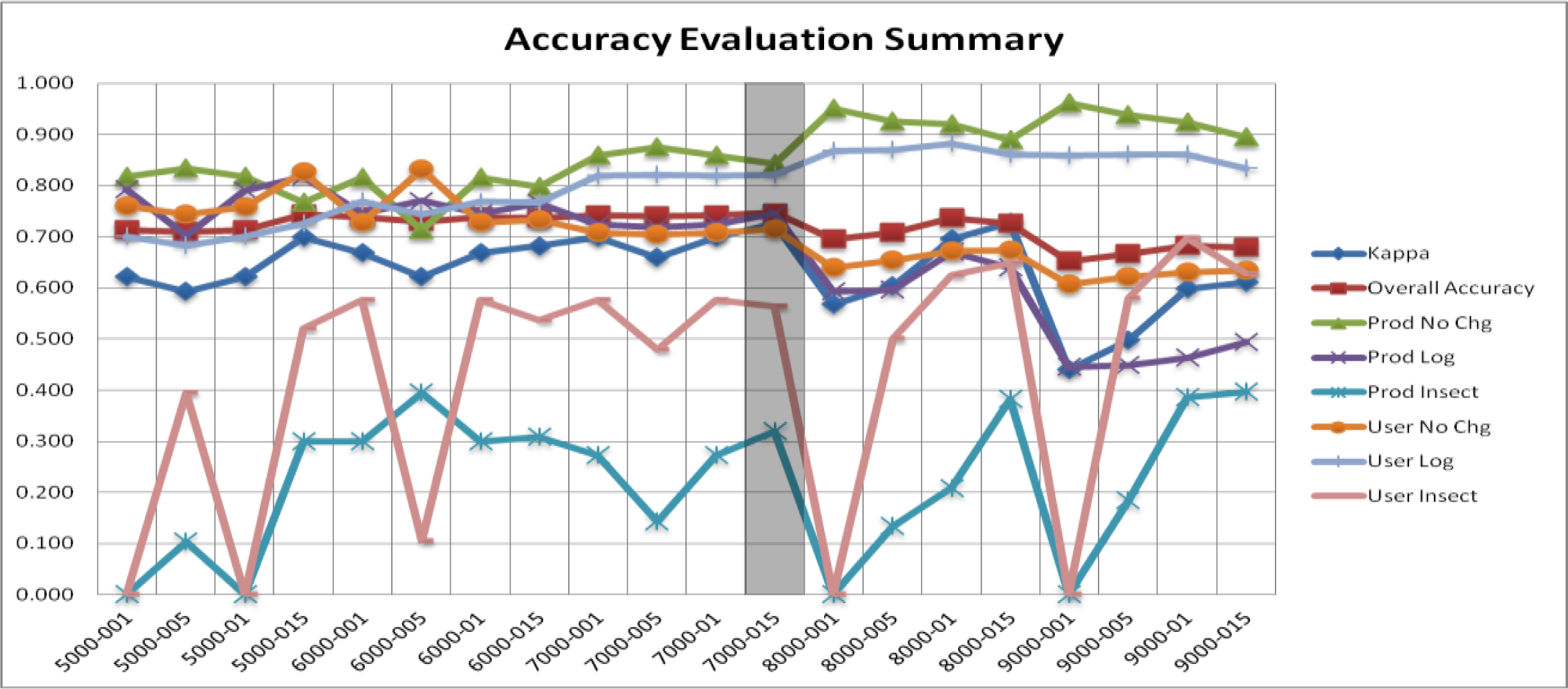
The ensemble approach removed user interpretation biases that can develop when deciding classification threshold values. Typically classifications are optimized through iterations to improve mapping accuracy. Our analysis sought to understand the sensitivity of DI’ to harvest and insect outbreaks, which is why we provide all of our accuracy evaluation results for all 20 maps in Figure 7. This approach allowed quantitative assessment of classification thresholds, while enhancing the understanding of commission and omission errors in disturbance type classification. We applied less than five threshold values to our classification trees. We could have applied more, although this increases the analyst evaluation effort. We performed disturbance evaluation per LTSS path/row and air-photo, and then, we aggregated this for the entire study region. Each of the four path/rows had different types and rates of disturbance, as we found from ancillary data. The classification ensemble approach across multiple path/rows enabled our sensitivity analysis of the spectral signatures to insect mortality and defoliation.

Our approach through multiple iterations in tree splits had a range in overall accuracy from 65% to 75%, with an average accuracy of 72%. Producer’s and user’s accuracy ranged from a maximum of 32% to 70% for insect disturbance, 60% to 76% for insect mortality and 82% to 88% for harvested forest, which was the dominant disturbance agent. Kappa varied from 44% to 73% when all the path/row evaluation data were combined.

Our automated classification approach revealed widespread disturbance dynamics similar to those reported in previous studies [36,42,44,86,87]. We selected the classification iteration with a logging threshold of −7000 and a p-value of 0.15 for the fit of DI’ for insect outbreaks to report our final results. This iteration had the highest summary evaluation metrics for overall accuracy and kappa for all path/rows (

Table 2. Validation statistics (Iteration 8 of 20), ensemble thresholding for logging (ΔDI > −7000) and insect outbreak (p < 0.15).

		Air Photo & Shapefile Reference Data
		No Change	Logging	Insect	Total	Map %
TM	No Change	684	181	91	956	56.1
Mapped Data	Logging	82	530	33	645	37.9
	Insect	45	0	58	103	6.0
	Total	811	711	182	1704	0.0
	%	47.6	41.7	10.7	0	0.0
Producer’s Accuracy		0.84	0.75	0.32
User’s Accuracy		0.72	0.82	0.56
Overall accuracy		75%
Kappa statistic		0.73

). However, insect disturbance had a higher user’s accuracy (40%) and producer’s accuracy (70%) for the classification iteration with a logging threshold of −9000 and a p-value of 0.1 for the fit of DI’. We did not select this iteration to report our mapping results, because the overall accuracy was 68% and the kappa was 60%.

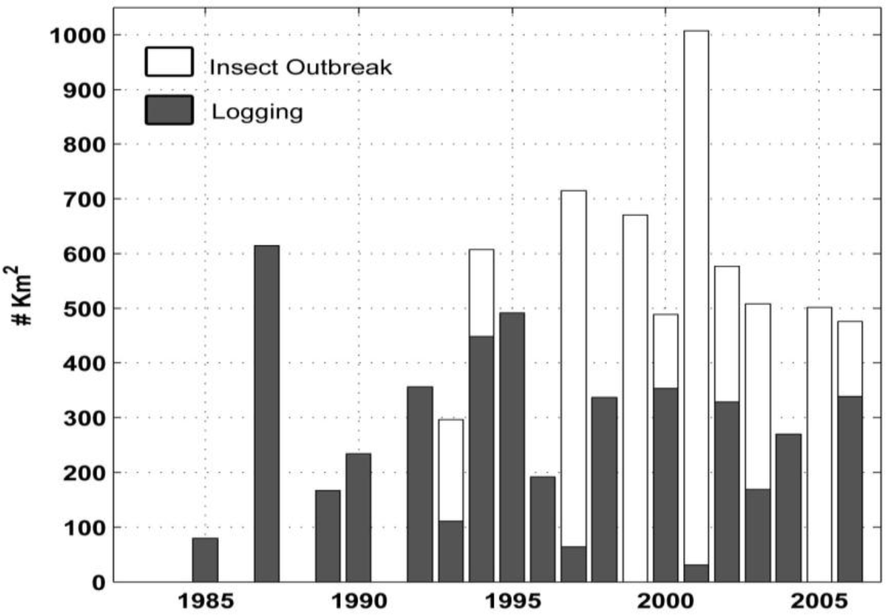
Our study region comprised 33,524 km² of forest, with a 1984 to 2006 disturbed area totaling 7349 km² (21.8% of the forest class). Disturbance due to logging was 4186 km², and insect outbreaks totaled 3163 km². We provide a summary of the disturbed area by year in Figure 8. Our approach captured the annual amount of insect outbreak disturbance over a multi-decadal period. Peak insect disturbance occurred in 2001 and covered 3% percent of the forested area that year. Logging disturbance was 44% of the total disturbance from 1993 to 2006. Classification accuracy of forest harvest was consistent between Landsat stacks throughout the study region.

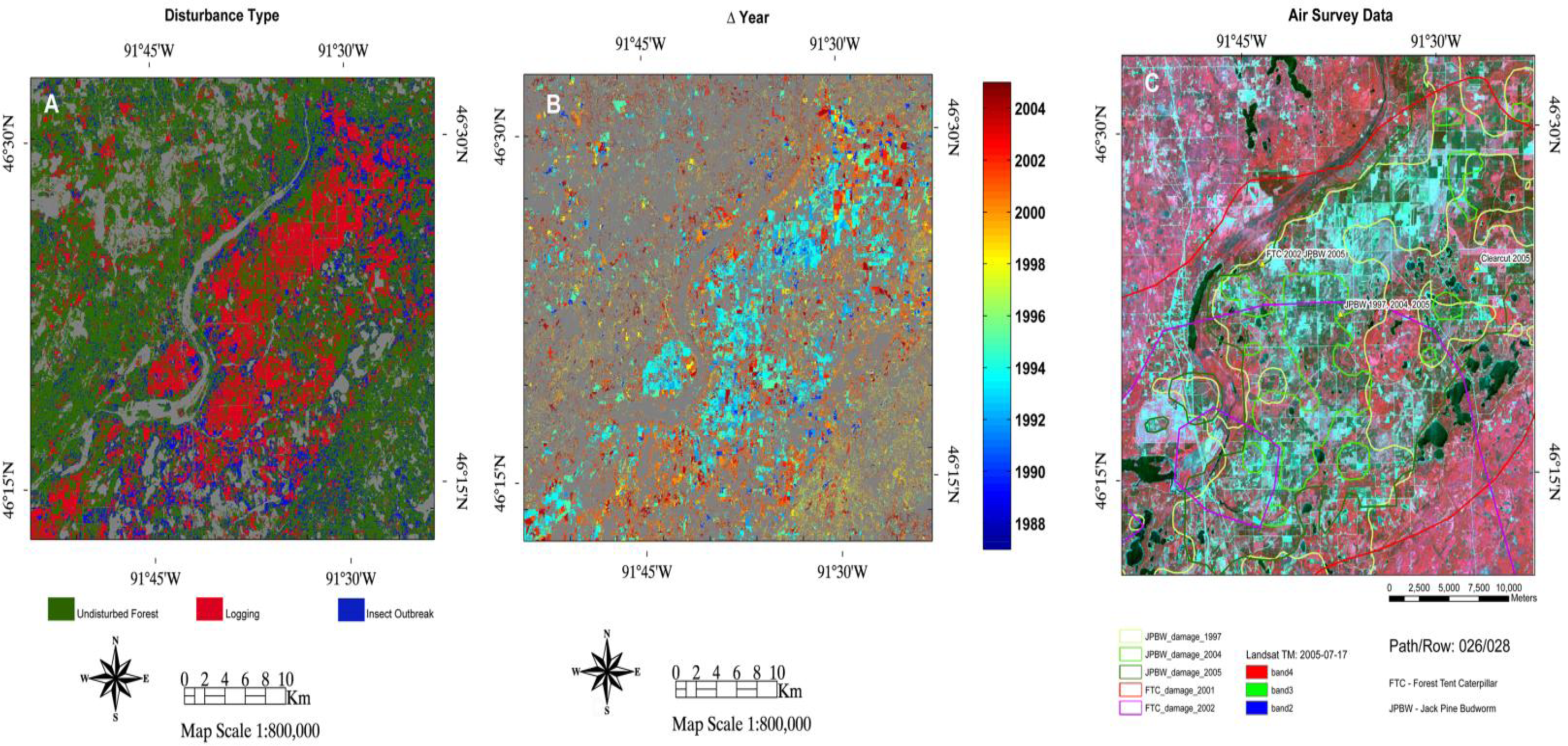
Insect disturbance was 56% of the total disturbance from 1993 to 2006. Classification evaluation was performed for each Landsat stack and aggregated for the entire study region. The greatest classification accuracy of insect disturbance was 72.1% user’s and 60.8% producer’s in Path 26, Row 28, Sawyer County, where mortality had occurred, leaving a long-term spectral signal that was marked in both air-photos and Landsat as compared to other Landsat stacks, where forest tent caterpillar defoliation was the dominant agent. This outbreak of jack pine budworm that caused mortality and increased forest fragmentation in the early 1990s has been studied thoroughly in the past [44,88,89], and insect disturbance has continued to be a problem to forest productivity in this region [90]. Forest tent caterpillar did not cause mortality and was identified over an outbreak period from 2000 to 2006 with aerial surveys. The producer’s and user’s accuracies of 31.9% and 56.3% overall for insect disturbance were low due to the difficulty of identifying forest tent caterpillar in air-photo validation data; and because of the limited time-series of the air-photo record. Note that one of the air-photo validation sites for Path 26, Row 28 corresponds to the area reported by air surveys as insect damage and mortality (Figure 1, yellow quadrangle center of map). We also believe Landsat has limited viability in capturing defoliating insects when the data is not available on a dense temporal basis. We provide accuracy assessment results for Path 26, Row 28 in Figure 9; note that the values reported for insect disturbance are higher than the averages for the entire study area for producer’s (32% vs. 63%) and user’s (70% vs. 72%) accuracies.

Insect outbreak invoking mortality in the pine barrens of Path 26, Row 28 during the mid-1990s and early 2000s followed by salvage logging produced the largest disturbance event of all four Landsat stacks. We verified this classification result with aerial survey data, and this outbreak was driven by jack pine budworm in white and red jack pine. This disturbance reoccurred with an outbreak of forest tent caterpillar in surrounding aspen-birch stands (Figure 10).

4. Discussion

We observed the growth of a forest disturbance at the 30-m scale that invoked a negative AVHRR NDVI trend at the 8-km scale. The productivity trend is difficult to determine without a growing season monthly time-series of Landsat to understand the spatial heterogeneity of disturbed and undisturbed stands at the 8-km scale. Disturbance heterogeneity is compounded because of reoccurring events and the growing extent of the disturbed area. We added a salvage logging class after we found that many forested pixels classified as insect disturbance were later classified as salvage logged. This was necessary because of the dynamic interaction of disturbances in this region. If we did not include a disturbance change class, our mapping accuracies for disturbance type would be greatly reduced.

The lack of peak growing season, cloud-free, annual growing season Landsat data dating back to 1984 is a limitation of this approach in this region, and the temporal density of the archive must be considered when applying our approach to classify forest disturbances. Multiple disturbance agents were identified, including a wide diversity of insects that reached outbreak populations, causing forest damage and mortality. We found insect damage or defoliation to be a widespread disturbance agent that cannot be captured with an LTSS disturbance index. We believe time series density has a direct impact on our results. The severity of the disturbance must be great enough to impose a multi-year change in surface reflectance with the statistical trend change approach. Image compositing and other more recent complex approaches by Brooks et al., 2013 [91], to use more multi-temporal Landsat data and remove phenology could prove useful in detecting degradation, thinning or insect defoliation events.

Disturbance rates in Path 26, Row 28 were consistent with other studies conducted over the same period of time. Radeloff et al., 1998, 2000, 2003 [42,44,87], found with Landsat that jack pine budworm through the mid-1990s decimated forest stands where, then, salvage logging took place. We found similar results and expanded our disturbance analysis to the surrounding LTSS path/rows where a strong long-term negative AVHRR NDVI anomaly existed. We found that prior methods captured disturbance dynamics well within this path/row, because of the strong spectral signatures of mortality and stand clearance. However, neighboring path/rows do not have this clear insect disturbance signature, probably due to the lack of jack pine mortality from budworm outbreak, and the widespread agent has been a defoliator, while most of the study region is deciduous forest. This poses additional mapping problems when using LTSS to define disturbance agents. One potential solution would be implementing multi-temporal high-resolution commercial data to map individual tree crowns. This has been successfully done by Wulder et al., 2008 [92], for monitoring mountain pine beetle mortality, but the Laurentian Forest region poses new challenges, because of the diversity of insects that can reach outbreak levels and the short-term damage signal that is not identifiable in the next growing season in deciduous forests. Future studies could utilize an archive of high resolution with LTSS to identify which insect outbreak types have discernible multi-temporal signals in LTSS. This has become more of a possibility with no-cost access to US commercial high-resolution imagery by US-funded researchers [93].

The heterogeneous nature of this landscape with evergreen and deciduous forest patches mixed with agriculture precludes defining one dominant cause of the decline, and we did not investigate changes in agriculture croplands, nor did we evaluate the influence of climate. Most of the AVHRR NDVI decline existed in forests. We believe that a progressive increase of the clear cut area at Landsat resolution has reduced the AVHRR NDVI. We did not investigate crop statistics to understand why NDVI has declined there and do not believe that the LTSS record is dense enough to capture changes in cropland productivity. Croplands did not exhibit strong negative trends as compared to forest classes. Additionally, widespread insect defoliation was observed with airborne sketch map surveys, but not captured in our disturbance classification, due to the limitations of LTSS density. An increased defoliated area could reduce NDVI through the reduction of leaf area and increased background soil reflectance, but we found that our algorithm and available Landsat data had limited to no sensitivity to these events.

This region was found to be a source of C, averaging 120 g·Cm²·yr⁻¹, observed by the WLEF tall tower in northern Wisconsin annualized over the years from 1997 to 2004 [94]. We believe that this tower is capturing the vegetation productivity decline observed by AVHRR. Once the disturbance rate subsides, this region under favorable climate conditions for growth should become a strong regrowth sink. Future remote sensing monitoring of disturbance rates could help understand how and when this transition occurs.

5. Conclusions

We believe negative NDVI trends in the Laurentian Forest observed by 8-km AVHRR are partially due from increased rates of disturbance. We initially had three questions when conducting this study and they included the following. First, were the long-term declines in forest productivity an error or real? From our classification results we believe the long-term AVHRR NDVI declines in the Laurentian Forest are associated with disturbances from insect outbreaks that caused defoliation and mortality, with salvage logging occurring in a large portion of dead forest stands. A large proportion of forest cover change has occurred over the same period of the NDVI decline, which implies that these disturbances are contributing to the change in NDVI. Our second question is, can an image classification algorithm be used on Landsat time-series data to extract forest disturbances reliably for a region with heterogeneous canopy cover? We found that a semi-automated decision tree approach can rapidly classify LTSS data for many path/rows, but only insect mortality and harvest have a strong enough spectral signal that can be identified when annual gaps in the time-series exist. Other approaches that use the full temporal record of Landsat and can exclude phenology may be able to detect more subtle events that are missed with this approach. Third, what dominant disturbance agent caused the NDVI decline at the coarse scale? We found a combination of disturbances from clear cut harvest, insect defoliation and mortality in patches of a heterogeneous landscape and suspect that they have reduced the large-scale productivity of the Laurentian Forest. The mixed composition of the land cover and change rates makes it difficult to determine one dominant agent, as it appears to be multiple disturbances occurring throughout the landscape at an increasing interval.

Typically, post-disturbance regrowth observed with AVHRR NDVI can take more than five years [12], although this can depend on biome, forest type, climate after disturbance and the available seed bank for regrowth. We did not find recovery of AVHRR NDVI throughout this region, but we did find successive forest disturbance within 30-m resolution Landsat data. AVHRR data provide insight to overall vegetation productivity and health for a region, but lack important disturbance dynamics that LTSS and in situ data can provide. Our algorithm is the first to our knowledge that tracks forest disturbances from one type to the next with a simple combination of spectral thresholding and trajectory analysis. Future studies need to incorporate disturbance dynamics that can be captured with dense LTSS data in biogeochemistry simulations to improve forest C accounting uncertainties.

References

1. Gower, S.T. Patterns and mechanisms of the forest carbon cycle. Ann. Rev. Environ. Res 2003, 28, 169–204. [Google Scholar]
2. Houghton, R.A.; Hackler, J.L.; Lawrence, K.T. The U.S. carbon budget: Contributions from land-use change. Science 1999, 285, 574–578. [Google Scholar]
3. Pacala, S.W.; Hurtt, G.C.; Baker, D.; Peylin, P.; Houghton, R.A.; Birdsey, R.A.; Heath, L.; Sundquist, E.T.; Stallard, R.F.; Ciais, P.; et al. Consistent land- and atmosphere-based U.S. carbon sink estimates. Science 2001, 292, 2316–2320. [Google Scholar]
4. Pan, Y.D.; Birdsey, R.A.; Fang, J.Y.; Houghton, R.; Kauppi, P.E.; Kurz, W.A.; Phillips, O.L.; Shvidenko, A.; Lewis, S.L.; Canadell, J.G.; et al. A large and persistent carbon sink in the world’s forests. Science 2011, 333, 988–993. [Google Scholar]
5. Canadell, J.G.; Pataki, D.; Gifford, R.; Houghton, R.A.; Lou, Y.; Raupach, M.R.; Smith, P.; Steffen, W. Saturation of the Terrestrial Carbon Sink. In Terrestrial Ecosystems in a Changing World; Canadell, J.G., Pataki, D., Pitelka, L., Eds.; Springer-Verlag: Berlin, Germany, 2007; pp. 59–78. [Google Scholar]
6. Plugge, D.; Kohl, M. Estimating carbon emissions from forest degradation: Implications of uncertainties and area sizes for a REDD+ MRV system. Can. J. For. Res 2012, 42, 1996–2010. [Google Scholar]
7. Sasaki, N.; Chheng, K.; Ty, S. Managing production forests for timber production and carbon emission reductions under the REDD plus scheme. Environ. Sci. Policy 2012, 23, 35–44. [Google Scholar]
8. Tucker, C.J.; Pinzon, J.E.; Brown, M.E.; Slayback, D.A.; Pak, E.W.; Mahoney, R.; Vermote, E.F.; Saleous, N.E. An Extended AVHRR 8-km NDVI Data Set Compatible with MODIS and SPOT Vegetation NDVI Data. Int. J. Remote Sens 2005, 26, 4485–4498. [Google Scholar]
9. Tucker, C.J. Red and photographic infrared linear combinations for monitoring vegetation. Remote Sens. Environ 1979, 8, 127–150. [Google Scholar]
10. Gamon, J.A.; Field, C.B.; Goulden, M.L.; Griffin, K.L.; Hartley, A.E.; Joel, G.; Penuelas, J.; Valentini, R. Relationships between NDVI, canopy structure, and photosynthesis in 3 Californian vegetation types. Ecol. Appl 1995, 5, 28–41. [Google Scholar]
11. Goetz, S.J.; Bunn, A.G.; Fiske, G.J.; Houghton, R.A. Satellite-observed photosynthetic trends across boreal North America associated with climate and fire disturbance. Proc. Natl. Acad. Sci. USA 2005, 102, 13521–13525. [Google Scholar]
12. Goetz, S.J.; Fiske, G.J.; Bunn, A.G. Using satellite time-series data sets to analyze fire disturbance and forest recovery across Canada. Remote Sens. Environ 2006, 101, 352–365. [Google Scholar]
13. Goetz, S.J.; Mack, M.C.; Gurney, K.R.; Randerson, J.T.; Houghton, R. Ecosystem responses to recent climate change and fire disturbance at northern high latitudes: Observations and model results contrasting northern Eurasia and North America. Environ. Res. Lett 2007, 2. [Google Scholar] [CrossRef]
14. Bunn, A.G.; Goetz, S.J. Trends in satellite-observed circumpolar photosynthetic activity from 1982 to 2003: The influence of seasonality, cover type, and vegetation density. Earth Interact 2006, 10, 1–19. [Google Scholar]
15. Bunn, A.G.; Goetz, S.J.; Fiske, G.J. Observed and predicted responses of plant growth to climate across Canada. Geophys. Res. Lett 2005, 32. [Google Scholar] [CrossRef]
16. Bunn, A.G.; Goetz, S.J.; Kimball, J.; Zhang, K. Northern high-latitude ecosystems respond to climate change. EOS Trans. AGU 2007, 88, 333–340. [Google Scholar]
17. Townshend, J.R.G. Remote Sensing-Global Local Views. In Horizons in Phys. Geography; Gregory, K., Gurnell, A., Eds.; MacMillian Publishers: London, UK, 1988. [Google Scholar]
18. Townshend, J.R.; Masek, J.G.; Huang, C.Q.; Vermote, E.F.; Gao, F.; Channan, S.; Sexton, J.O.; Feng, M.; Narasimhan, R.; Kim, D.; et al. Global characterization and monitoring of forest cover using Landsat data: opportunities and challenges. Int. J. Digit. Earth 2012, 5, 373–397. [Google Scholar]
19. Miller, J.D.; Thode, A.E. Quantifying burn severity in a heterogenous landscape with a relative version of the delta Normalized Burn Ratio (dNBR). Remote Sens. Environ 2007, 109, 66–80. [Google Scholar]
20. Schroeder, T.A.; Wulder, M.A.; Healey, S.P.; Moisen, G.G. Mapping wildfire and clearcut harvest disturbances in boreal forests with Landsat time series data. Remote Sens. Environ 2011, 115, 1421–1433. [Google Scholar]
21. Goodwin, N.R.; Coops, N.C.; Wulder, M.A.; Gillanders, S.; Schroeder, T.A.; Nelson, T. Estimation of insect infestation dynamics using a temporal sequence of Landsat data. Remote Sens. Environ 2008, 112, 3680–3689. [Google Scholar]
22. Kurz, W.A.; Apps, M.J. Developing Canada’s national forest carbon monitoring, accounting and reporting systems to meet the reporting requirements of the Kyoto Protocol. Mitig. Adapt. Strat. Glob 2006, 11, 33–43. [Google Scholar]
23. Tucker, C.J.; Grant, D.M.; Dykstra, J.D. NASA’s global orthorectified Landsat data set. Photogramm. Eng. Remote Sens 2004, 70, 313–322. [Google Scholar]
24. Neigh, C.S.R.; Tucker, C.J.; Townshend, J.R.G. North American vegetation dynamics observed with multi-resolution satellite data. Remote Sens. Environ 2008, 112, 1749–1772. [Google Scholar]
25. Masek, J.G.; Huang, C.Q.; Wolfe, R.; Cohen, W.; Hall, F.; Kutler, J.; Nelson, P. North American forest disturbance mapped from a decadal Landsat record. Remote Sens. Environ 2008, 112, 2914–2926. [Google Scholar]
26. Goward, S.N.; Masek, J.G.; Cohen, W.; Moisen, G.; Collatz, G.J.; Healey, S.; Houghton, R.; Huang, C.; Kennedy, R.; Law, B.; et al. Forest disturbance and North American carbon flux. EOS Trans. AGU 2008, 89, 105–116. [Google Scholar]
27. Kennedy, R.E.; Cohen, W.B.; Schroeder, T.A. Trajectory-based change detection for automated characterization of forest disturbance dynamics. Remote Sens. Environ 2007, 110, 370–386. [Google Scholar]
28. Schroeder, T.A.; Wulder, M.A.; Healey, S.P.; Moisen, G.G. Detecting post-fire salvage logging from Landsat change maps and national fire survey data. Remote Sens. Environ 2012, 122, 166–174. [Google Scholar]
29. Huang, C.Q.; Coward, S.N.; Masek, J.G.; Thomas, N.; Zhu, Z.L.; Vogelmann, J.E. An automated approach for reconstructing recent forest disturbance history using dense Landsat time series stacks. Remote Sens. Environ 2010, 114, 183–198. [Google Scholar]
30. Coops, N.; Wulder, M.A. Estimating the reduction in gross primary production due to mountain pine beetle infestation using satellite observations. Int. J. Remote Sens 2010, 31, 2129–2138. [Google Scholar]
31. Miller, J.D.; Knapp, E.E.; Key, C.H.; Skinner, C.N.; Isbell, C.J.; Creasy, R.M.; Sherlock, J.W. Calibration and validation of the relative differenced Normalized Burn Ratio (RdNBR) to three measures of fire severity in the Sierra Nevada and Klamath Mountains, California, USA. Remote Sens. Environ 2009, 113, 645–656. [Google Scholar]
32. Munyati, C.; Kabanda, T.A. Using multitemporal Landsat TM imagery to establish land use pressure induced trends in forest and woodland cover in sections of the Soutpansberg Mountains of Venda region, Limpopo Province, South Africa. Reg. Environ. Chang 2009, 9, 41–56. [Google Scholar]
33. Pax-Lenney, M.; Woodcock, C.E.; Macomber, S.A.; Gopal, S.; Song, C. Forest mapping with a generalized classifier and Landsat TM data. Remote Sens. Environ 2001, 77, 241–250. [Google Scholar]
34. Song, C.; Schroeder, T.A.; Cohen, W.B. Predicting temperate conifer forest successional stage distributions with multitemporal Landsat Thematic Mapper imagery. Remote Sens. Environ 2007, 106, 228–237. [Google Scholar]
35. Soverel, N.O.; Perrakis, D.D.B.; Coops, N.C. Estimating burn severity from Landsat dNBR and RdNBR indices across western Canada. Remote Sens. Environ 2010, 114, 1896–1909. [Google Scholar]
36. Radeloff, V.C.; Mladenoff, D.J.; Boyce, M.S. Detecting jack pine budworm defoliation using spectral mixture analysis: Separating effects from determinants. Remote Sens. Environ 1999, 69, 156–169. [Google Scholar]
37. Stinson, G.; Kurz, W.A.; Smyth, C.E.; Neilson, E.T.; Dymond, C.C.; Metsaranta, J.M.; Boisvenue, C.; Rampley, G.J.; Li, Q.; White, T.M.; et al. An inventory-based analysis of Canada’s managed forest carbon dynamics, 1990 to 2008. Glob. Chang. Biol 2011, 17, 2227–2244. [Google Scholar]
38. Kurz, W.A.; Dymond, C.C.; Stinson, G.; Rampley, G.J.; Neilson, E.T.; Carroll, A.L.; Ebata, T.; Safranyik, L. Mountain pine beetle and forest carbon feedback to climate change. Nature 2008, 452, 987–990. [Google Scholar]
39. Hais, M.; Jonasova, M.; Langhammer, J.; Kucera, T. Comparison of two types of forest disturance using multitemporal Landsat TM/ETM+ imagery and field vegetation data. Remote Sens. Environ 2009, 113, 835–845. [Google Scholar]
40. Stueve, K.M.; Housman, I.W.; Zimmerman, P.L.; Nelson, M.D.; Webb, J.B.; Perry, C.H.; Chastain, R.A.; Gormanson, D.D.; Huang, C.; Healey, S.P.; et al. Snow-covered Landsat time series stacks improve automated disturbance mapping accuracy in forested landscapes. Remote Sens. Environ 2011, 115, 3203–3219. [Google Scholar]
41. Hais, M.; Kucera, T. Surface temperature change of spruce forest as a result of bark beetle attack: remote sensing and GIS approach. Eur. J. For. Res 2008, 127, 327–336. [Google Scholar]
42. Radeloff, V.C.; Mladenoff, D.J.; Boyce, M.S. Effects of Interacting disturbances on landscape patterns: budworm defoliation and salavage logging. Ecol. Appl 2000, 10, 233–247. [Google Scholar]
43. Grossmann, E.B.; Mladenoff, D.J. Open woodland and savanna decline in a mixed-disturbance landscape (1938 to 1998) in nthe Northwest Wisconsin (USA) Sand Plain. Landsc. Ecol 2007, 22, 43–55. [Google Scholar]
44. Radeloff, V.C.; Mladenoff, D.J.; Boyce, M.S. The changing relation of landscape patterns and jack pine budworm populations during an outbreak. Oikos 2003, 90, 417–430. [Google Scholar]
45. Reinikainen, M.; D’Amato, A.W.; Fraver, S. Repeated insect outbreaks promote multi-cohort aspen mixedwood forests in northern Minnesota, USA. For. Ecol. Manag 2012, 266, 148–159. [Google Scholar]
46. Holben, B. Characteristics of maximum-value composite images from temporal AVHRR data. Int. J. Remote Sens 1986, 7, 1417–1434. [Google Scholar]
47. Brown, M.E.; Pinzon, J.E.; Tucker, C.J. New vegetation index data set available to monitor global change. EOS Trans. AGU 2004, 85, 565–569. [Google Scholar]
48. Pinzon, J.E.; Brown, M.E.; Tucker, C.J. EMD correction of orbital drift artifacts in satellite data stream. Interd. Math Sci 2005, 5, 167–186. [Google Scholar]
49. Slayback, D.; Pinzon, J.; Los, S.; Tucker, C.J. Northern hemisphere photosynthetic trends 1982–99. Glob. Chang. Biol 2003, 9, 1–15. [Google Scholar]
50. Eidenshink, J.; Schwind, B.; Brewer, K.; Zhu, Z.; Qualye, B.; Howard, S. A project for monitoring trends in burn severity. Fire Ecol 2007, 3, 3–21. [Google Scholar]
51. USGS Global Visualization Viewer. Available online: http://glovis.usgs.gov (accessed on 17 March 2014).
52. Crist, E.P.; Cicone, R.C. Application of the Tasseled Cap concept to simulated Thematic Mapper data. Photogramm. Eng. Remote Sens 1984, 50, 343–352. [Google Scholar]
53. Guild, L.S.; Cohen, W.B.; Kauffman, J.B. Detection of deforestation and land conversion in Rondonia, Brazil using change detection techniques. Int. J. Remote Sens 2004, 25, 731–750. [Google Scholar]
54. Healey, S.P.; Yang, Z.Q.; Cohen, W.B.; Pierce, D.J. Application of two regression-based methods to estimate the effects of partial harvest on forest structure using Landsat data. Remote Sens. Environ 2006, 101, 115–126. [Google Scholar]
55. Homer, C.; Dewitz, J.; Fry, J.; Coan, M.; Hossain, N.; Larson, C.; Herold, N.; McKerrow, A.; VanDriel, J.N.; Wickham, J. Completion of the 2001 National Land Cover Database for the conterminous United States. Photogramm. Eng. Remote Sens 2007, 73, 337–341. [Google Scholar]
56. Vieira, I.C.G.; de Almeida, A.S.; Davidson, E.A.; Stone, T.A.; de Carvalho, C.J.R.; Guerrero, J.B. Classifying successional forests using Landsat spectral properties and ecological characteristics in eastern Amazonia. Remote Sens. Environ 2003, 87, 470–481. [Google Scholar]
57. Irish, R.R.; Barker, J.L.; Goward, S.N.; Arvidson, T. Characterization of the Landsat-7 ETM+ automated cloud-cover assessment (ACCA) algorithm. Photogramm. Eng. Remote Sens 2006, 72, 1179–1188. [Google Scholar]
58. Masek, J.G.; Vermote, E.F.; Saleous, N.E.; Wolfe, R.; Hall, F.G.; Huemmrich, K.F.; Gao, F.; Kutler, J.; Lim, T. A Landsat Surface Reflectance Dataset for North America, 1990–2000. IEEE Geosci. Remote Sens 2006, 3, 68–72. [Google Scholar]
59. Cohen, W.B.; Spies, T.A.; Alig, R.J.; Oetter, D.R.; Maiersperger, T.K.; Fiorella, M. Characterizing 23 years (1972–95) of stand replacement disturbance in western Oregon forests with Landsat imagery. Ecosystems 2002, 5, 122–137. [Google Scholar]
60. Hilker, T.; Wulder, M.A.; Coops, N.C.; Linke, J.; McDermid, G.; Masek, J.G.; Gao, F.; White, J.C. A new data fusion model for high spatial- and temporal-resolution mapping of forest disturbance based on Landsat and MODIS. Remote Sens. Environ 2009, 113, 1613–1627. [Google Scholar]
61. Townshend, J.R.G.; Justice, C.O.; Gurney, C.; McManus, J. The Impact of Misregistration on Change Detection. IEEE Trans. Geosci. Remote Sens 1992, 30, 1054–1060. [Google Scholar]
62. WisconsinView. Available online: ftp://ftp.ssec.wisc.edu/pub/wisconsinview (accessed on 17 March 2014).
63. USGS Monitoring Trends in Burn Severity (MTBS). Available online: www.mtbs.gov (accessed on 17 March 2014).
64. Epting, J.; Verbyla, D.; Sorbel, B. Evaluation of remotely sensed indices for assessing burn severity in interior Alaska using Landsat TM and ETM+. Remote Sens. Environ 2005, 96, 328–339. [Google Scholar]
65. United States Department of Agriculture. Forest Insect and Disease Conditions in the United States, 2008; USDA: Washington, DC, USA, 2009; p. 37. [Google Scholar]
66. Klien, W.H.; Tunnock, S.; Ward, J.G.D.; Knopf, J.A.E. Aerial Sketchmapping; USDA: Fort Collins, CO, USA, 1983; p. 15. [Google Scholar]
67. McConnell, T.; Johnson, E.; Burns, B. A Guide to Conducting Aerial Sketchmap Surveys; USDA: Fort Collins, CO, USA, 2000; p. 88. [Google Scholar]
68. Biging, G.; Congalton, R.G. Advances in Forest Inventory Using Advanced Digital Imagery. In Proceedings of Global Natural Research Monitoring and Assessments: Preparing for the 21st Century, Venice, Italy, 24–30 September 1989; pp. 1241–1249.
69. Congalton, R.G. A review of assessing the accuracy of classifications of remotely sensed data. Remote Sens. Environ 1991, 37, 35–46. [Google Scholar]
70. Lu, D.; Weng, Q. A survey of image classification methods and techniques for improving classification performance. Int. J. of Remote Sens 2007, 28, 823–870. [Google Scholar]
71. Muller, S.V.; Walker, D.A.; Nelson, F.E.; Auerbach, N.A.; Bockheim, J.G.; Guyer, S.; Sherba, D. Accuracy assessment of a land-cover map of the Kuparuk River Basin, Alaska: Considerations for remote regions. Photogramm. Eng. Remote Sens 1998, 64, 619–628. [Google Scholar]
72. Stehman, S.V.; Wickham, J.D.; Fattorini, L.; Wade, T.D.; Baffetta, F.; Smith, J.H. Estimating accuracy of land-cover composition from two-stage cluster sampling. Remote Sens. Environ 2009, 113, 1236–1249. [Google Scholar]
73. Congalton, R.G. A Comparison of sampling schemes used in generating error matrices for assessing the accuracy of maps generated from remotely sensed data. Photogramm. Eng. Remote Sens 1988, 54, 593–600. [Google Scholar]
74. Chen, D.M.; Wei, H. The effect of spatial autocorrelation and class proportion on the accuracy measures from different sampling designs. ISPRS J. Photogramm. Remote Sens 2009, 64, 140–150. [Google Scholar]
75. Franklin, S.E.; Peddle, D.R.; Wilson, B.A.; Blodgett, C.F. Pixel sampling of remotely sensed digital imagery. Comput Geosci 1991, 17, 759–775. [Google Scholar]
76. Stehman, S.V. Sampling designs for accuracy assessment of land cover. Int. J. Remote Sens 2009, 30, 5243–5272. [Google Scholar]
77. Stehman, S.V.; Sohl, T.L.; Loveland, T.R. Statistical sampling to characterize recent United States land-cover change. Remote Sens. Environ 2003, 86, 517–529. [Google Scholar]
78. Loveland, T.R.; Sohl, T.L.; Stehman, S.V.; Gallant, A.L.; Sayler, K.L.; Napton, D.E. A strategy for estimating the rates of recent United States land-cover changes. Photogramm. Eng. Remote Sens 2002, 68, 1091–1099. [Google Scholar]
79. Congalton, R. Putting the Map Back in Map Accuracy Assessment. In Remote Sensing and GIS Accuracy Assessment; Lunetta, R.S., Lyon, J.G., Eds.; CRC Press: Boca Raton, FL, USA, 2004; pp. 1–11. [Google Scholar]
80. Congalton, R.G.; Green, K. Assessing the accuracy of remotely sensed data: Principles and practices; CRC Press: Boca Raton, FL, USA, 1998. [Google Scholar]
81. Cohen, J. Weighted Kappa: Nominal scale agreement with provision for scaled disagreement or partial credit. Psychol Bull 1968, 70, 213–220. [Google Scholar]
82. Story, M.; Congalton, R. Accuracy assessment: A user’s perspective. Photogramm. Eng. Remote Sens 1986, 52, 397–399. [Google Scholar]
83. Stenback, J.M.; Congalton, R.G. Using thematic mapper imagery to examine forest understory. Photogramm. Eng. Remote Sens 1990, 56, 1285–1290. [Google Scholar]
84. Ruefenacht, B.; Finco, M.V.; Nelson, M.D.; Czaplewski, R.; Helmer, E.H.; Blackard, J.A.; Holden, G.R.; Lister, A.J.; Salajanu, D.; Weyermann, D.; et al. Conterminous US and Alaska forest type mapping using forest inventory and analysis data. Photogramm. Eng. Remote Sens 2008, 74, 1379–1388. [Google Scholar]
85. Nagol, J.R.; Vermote, E.F.; Prince, S.D. Effects of atmospheric variation on AVHRR NDVI data. Remote Sens. Environ 2009, 113, 392–397. [Google Scholar]
86. Powell, S.L.; Cohen, W.B.; Healey, S.P.; Kennedy, R.E.; Moisen, G.G.; Pierce, K.B.; Ohmann, J.L. Quantification of live aboveground forest biomass dynamics with Landsat time-series and field inventory data: A comparison of empirical modeling approaches. Remote Sens. Environ 2010, 114, 1053–1068. [Google Scholar]
87. Radeloff, V.C.; Mladenoff, D.J.; Boyce, M.S. Jack Pine Budworm Defoliation Monitoring and Modelling Using Spectral Mixture Analysis. In Proceedings of the 27th International Symposium on Remote Sensing of Environment, Tromso, Norway, 8–12 June 1998; pp. 644–647.
88. Bresee, M.K.; Le Moine, J.; Mather, S.; Brosofske, K.D.; Chen, J.Q.; Crow, T.R.; Rademacher, J. Disturbance and landscape dynamics in the Chequamegon National Forest Wisconsin, USA, from 1972 to 2001. Landsc. Ecol 2004, 19, 291–309. [Google Scholar]
89. Zhu, J.; Rasmussen, J.G.; Moller, J.; Aukema, B.H.; Raffa, K.F. Spatial-temporal modeling of forest gaps generated by colonization from below- and above-ground bark beetle species. J. Am. Stat. Assoc 2008, 103, 162–177. [Google Scholar]
90. Cook, B.D.; Bolstad, P.V.; Naesset, E.; Anderson, R.S.; Garrigues, S.; Morisette, J.T.; Nickeson, J.; Davis, K.J. Using LiDAR and quickbird data to model plant production and quantify uncertainties associated with wetland detection and land cover generalizations. Remote Sens. Environ 2009, 113, 2366–2379. [Google Scholar]
91. Brooks, E.B.; Wynne, R.H.; Thomas, V.A.; Blinn, C.E.; Coulston, J.W. On-the-fly massively multitemporal change detection using statistical quality control charts and Landsat data. IEEE Trans. Geosci. Remote Sens 2013, 52, 1–17. [Google Scholar]
92. Wulder, M.A.; Ortlepp, S.M.; White, J.C.; Coops, N.C.; Coggins, S.B. Monitoring the impacts of mountain pine beetle mitigation. Forest Ecol. Manag 2009, 258, 1181–1187. [Google Scholar]
93. Neigh, C.S.R.; Masek, J.G.; Nickeson, J. High-resolution satellite data open for government research. EOS Trans. AGU 2013, 94, 121–123. [Google Scholar]
94. Ricciuto, D.M.; Butler, M.P.; Davis, K.J.; Cook, B.D.; Bakwin, P.S.; Andrews, A.; Teclaw, R.M. Causes of interannual variability in ecosystem-atmosphere CO2 exchange in a northern Wisconsin forest using a Bayesian model calibration. Agric. For. Meteorol 2008, 148, 309–327. [Google Scholar]
Figure 1. Global Inventory Modeling and Mapping Studies (GIMMS) Normalized Difference Vegetation Index (NDVI) negative trends indicated with black quadrangles overlaid upon one date of Landsat false-color composite images (4,3,2, red, green, blue). Insect disturbance from aerial survey data is overlaid in green (damage) and orange (mortality). Red open polygons indicate the monitoring trends in burning severity (MTBS) burned area, and yellow open polygons indicate validation data locations.
Remotesensing 06 02782f1
Figure 2. Illustration of annual Landsat classification used to understand disturbances on forest productivity trends. NLCD, National Land Cover Database; LEDAPS, Landsat Ecosystem Disturbance Adaptive Processing System; DI’, Disturbance Index.
Remotesensing 06 02782f2
Figure 3. Landsat day of year (DOY) acquisitions by path and row. We used AVHRR data to select peak growing season images with minimum cloud cover.
Remotesensing 06 02782f3
Figure 4. The geographic extent of forest cover types throughout the study region. The black open polygon indicates the Landsat image bounds, and yellow quadrangles indicate the locations of high-resolution validation data.
Remotesensing 06 02782f4
Figure 5. (A) AVHRR NDVI anomaly histogram stacked by forest species cover type, with the inset pie chart showing the proportion of the area by species cover type. (B) AVHRR NDVI anomaly stacked by 2001 NLCD types with the inset pie chart depicting the proportion of cover types with a statistically significant NDVI trend.
Remotesensing 06 02782f5
Figure 6. The growing season, May to September, negative GIMMS AVHRR NDVI g trend (the bold green line is the three-year running average) from a sample of pixels (indicated in the plot title) in WRS path/row locations with Landsat dates used in the classification (red vertical lines). The standard deviation for the sampled pixels is shown at the bottom of each plot with black circles.
Remotesensing 06 02782f6
Figure 7. Accuracy evaluation summary results from all iterations of adjusted classification tree splits for each path/row. We selected iteration 7000-015 (DI’ threshold of −7000 and p-value of 0.015; the vertical grey shaded portion of the plot) because it had the greatest combination of evaluation metrics, including overall accuracy, kappa statistic and producer’s and user’s accuracies for all path/rows.
Remotesensing 06 02782f7
Figure 8. Sum of study region annual area disturbed by insects and logging.
Remotesensing 06 02782f8
Figure 9. Accuracy evaluation summary results for Path 26, Row 28. Results show iterations of adjusted classification tree splits.
Remotesensing 06 02782f9
Figure 10. Example of disturbance classification evaluation and change results for a subset area of Path 26, Row 28. (A) The results of the land cover change classification by disturbance type. (B) The classified Landsat stack change year. Most of the insect outbreak disturbance in this subset was reclassified as salvage logging from the rapid decline in DI’ after it was classified as an insect outbreak. (C) A Landsat false color composite of the disturbed site showing the extent of the air survey data of jack pine budworm (Choristoneura pinus) and forest tent caterpillar (Malacosoma disstria).
Remotesensing 06 02782f10