Extraction of Urban Power Lines from Vehicle-Borne LiDAR Data

Abstract

Airborne LiDAR has been traditionally used for power line cruising. Nevertheless, data acquisition with airborne LiDAR is constrained by the complex environments in urban areas as well as the multiple parallel line structures on the same power line tower, which means it is not directly applicable to the extraction of urban power lines. Vehicle-borne LiDAR system has its advantages upon airborne LiDAR and this paper tries to utilize vehicle-borne LiDAR data for the extraction of urban power lines. First, power line points are extracted using a voxel-based hierarchical method in which geometric features of each voxel are calculated. Then, a bottom-up method for filtering the power lines belonging to each power line is proposed. The initial clustering and clustering recovery procedures are conducted iteratively to identify each power line. The final experiment demonstrates the high precision of this technique.

1. Introduction

Power lines are important components of the power sector and their monitoring has significant roles in various areas, such as power line patrols [1], electric net design and upgrading [2], and the professional analysis of electricity [3]. The detection and monitoring of power lines can provide strong support for electric circuit management and decision-making [4]. Airborne LiDAR is a rapid, efficient, and high-precision method for obtaining spatial data [5,6], and it has been accepted widely by the power sector as the principle tool for monitoring power lines [1]. Several methods have been proposed for extracting power lines from airborne LiDAR data. For example, Melzer and Briese [7] extracted power line points using a bottom-up strategy and applied the Hough transform iteratively to identify each single power line. McLaughlin [8] classified power line points based on their point features using a Gaussian mixture model. Based on the slope and peak values, Liu et al. [9] performed filtering and detected the power lines by combining this approach with the Hough transform. Yu et al. [10] used an angle-based filtering method based on point filtering to extract the point features from non-ground points. Liang et al. [11] selected power line points manually and introduced a point filtering algorithm based on K-dimension (KD) trees to identify each power line, while a parabolic model was used to fit the power line points. Jwa et al. [12] used the Hough transform, feature eigenvectors, and point density in a comprehensive approach to extract power line points, and a piecewise catenary curve model-growing algorithm was proposed to identify the points in each power line. Based on this method, Jwa and Sohn [13] conducted an experiment using a high density point cloud, which was acquired at a height of 120 m, and good results were obtained.

Airborne LiDAR are usually carried by an airplane or a helicopter. During scanning, the system operates on an airplane flying at about 1000 m or a helicopter flying at 200–300 m [14,15]. When a same airborne LiDAR system acquires data in a fixed gesture, the point distance will be greater with increased height and vice versa [13]. Thus, when the points are obtained at 120 m, the point distance along power lines is only 0.3 m. In Jwa and Sohn [16], the points were obtained at a height of 400 m, so the point distance reached 1 m. To obtain sufficient power line points, the airborne LiDAR system is generally mounted on a helicopter, which has a relatively low flying height (60–150 m) [17]. Good results can be obtained using a low-flying helicopter for large-scale power line inspections. However, the buildings can be extremely high in urban areas, even exceeding the general scanning height of a helicopter. This makes the working environment of the helicopter complicated and dangerous [18]. However, the scarcity of land in urban areas means that multiple parallel power line structures (as shown in Figure 1) are used to reduce the land coverage of the transmission corridors. Airborne LiDAR systems obtain data at a constant off-nadir scan angle [19], so the power line information can only be detected from the first cross-arm whereas the others are missed. Thus, it is necessary to explore new data sources and to develop new methods to overcome the drawbacks of airborne LiDAR data during urban power line detection.

Vehicle-borne LiDAR, which is an emerging mobile mapping system, can capture road surface features rapidly from high-speed vehicles [20–22]. At present, vehicle-borne LiDAR is used widely for the extraction and modeling of roads [23], architecture [24], trees [25], streetlights [26], and pole-like objects [20]. However, there have been very few studies of power line extraction based on vehicle-borne LiDAR data. Lam et al. extracted 3D road data using Kalman Filter and then recognized post structure using line RANSAC (Random sample consensus) followed by a line least squares fit. After obtaining power line posts, they conducted their searches in an efficient way by looking at points inside a 3D bounding box between two consecutive power line posts [27]. This paper focuses on the extraction of road data and extracted power line points as attached elements. They did not make any attempt to identify single power lines. Ou et al. [18] made an attempt to extract power lines from vehicle-borne LiDAR data. Based on a height constraint and the Hough transform, they extracted power line points and then fitted the power lines using a parabolic function. This experiment showed that it is feasible to use vehicle-borne LiDAR data for detecting and inspecting power lines. Indeed, vehicle-borne LiDAR data can be applied effectively to power line extraction (particularly urban power lines) because of the following characteristics. (1) Urban road networks are well developed and the power lines are often distributed along the roads, which makes them accessible for vehicle-borne LiDAR; (2) During data collection, vehicle-borne LiDAR system is only a few meters from the power lines. The extracted point density is relatively high and the average point distance for the power lines can reach the centimeter-level; (3) vehicle-borne LiDAR captures data from a side view, which facilitates the acquisition of relatively complete point datasets from multiple parallel line views; (4) Data acquisition with vehicle-borne LiDAR systems costs less than that with airborne LiDAR. Vehicle-borne LiDAR systems can also be used to detect power lines at any time, so they have the capacity to provide an efficient tool for managing the power line accidents.

Based on these considerations, the present study used vehicle-borne LiDAR data to develop an urban power line extraction method. As noted above, there are many methods for power line extraction from airborne LiDAR data, but methods based on vehicle-borne LiDAR data are still rare. Airborne LiDAR system acquires data from above surface objects, where one plane coordinate (x, y) corresponds to one z value. In other words, airborne LiDAR data is just like 2D plane points with Z values. However, vehicle-borne LiDAR system acquires data in a side view so the plane coordinate (x, y) corresponds to several z values, which makes it real three-dimensional (3-D) points [28]. Thus, the point processing algorithms designed for airborne LiDAR data cannot be used directly to deal with vehicle-borne LiDAR points [21,29]. Therefore, it is necessary to search for the features that are fit for the extraction of power line points in vehicle-borne LiDAR data. In this paper, a voxel-based hierarchical method for the accurate extraction of power lines points is developed. Based on the extracted power line points, a bottom-up method is introduced for the identification of points belonging to each power line.

2. Data Acquisition

2.1. SSW Vehicle-Borne Modeling and Survey System

SSW vehicle-borne modeling and survey system is developed by Capital Normal University and Beijing Geo-Vision Technology Limited Liability Company. This system includes 360 degree laser scanner, IMU and GPS, CCD camera, etc. This system adopts the laser scanner with long range, high accuracy, large FOV, and IMU with high accuracy. Compared with similar products, the advantages of SSW are as follows: short initial time span, easy operation procedure, high accuracy, automatic classification and modeling. Its main technical parameters are as follows: point frequency 50–200 KHZ, lines per second 50–100 HZ, 360° scanning cope, surveying range 3–300 m, reflectance 80%, divergence angle 0.3 marc and relative measurement accuracy 2 cm/100 m.

2.2. Experimental Data

The vehicle-borne LiDAR data was obtained around Nanjing Olympic Sports Center, China, and they covered an area of about 4000 × 4000 m². The survey occurred in 2011 and a topographic map of 1:500 was used for correction. The size of acquired data was around 30 GB. Region A in Figure 2a was selected as the experimental area, which covered 800 × 200 m², with 30 million points and the average point distance along the power lines was 7 cm as shown in Figure 2b.

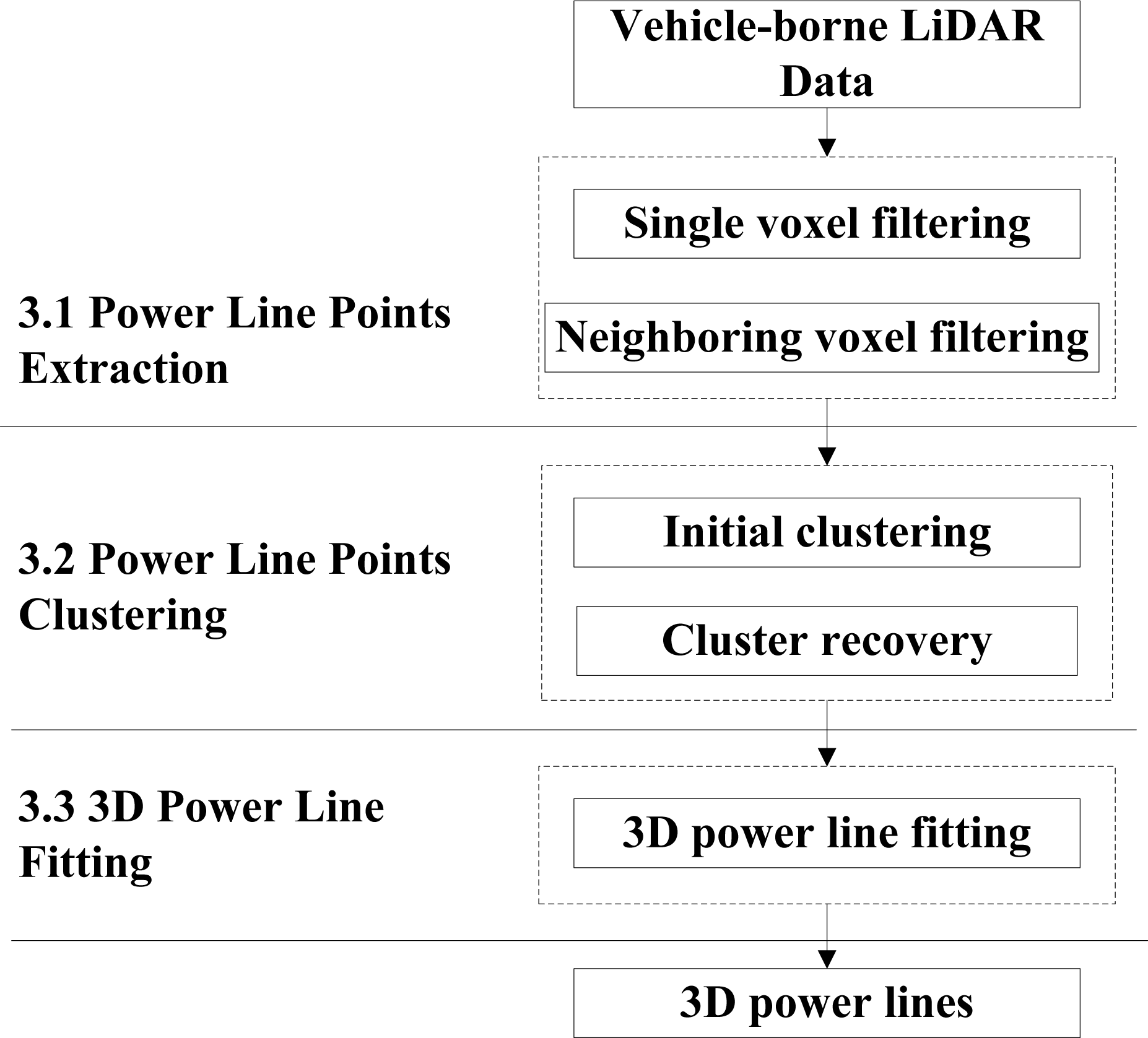
3. Method for Extracting Power Lines from Vehicle-Borne LiDAR Data

In general, power line extraction from LiDAR point clouds involves three procedures: extraction of power line points, clustering single power line points, and 3-D power line fitting. Thus, a voxel-based hierarchical method is developed for extracting power line points from vehicle-borne LiDAR data, where the two hierarchical layers are single voxel filtering and neighboring voxel filtering. Next, a bottom-up method is introduced for clustering power line points to deal with multiple parallel power line structures in urban areas. The initial clustering and clustering recovery procedures are conducted iteratively to identify each power line. Finally, a polynomial function is used to fit the power line points to obtain the 3-D power lines. The specific procedures used in this method are shown in Figure 3.

3.1. Power Line Points Extraction

Vehicle-borne LiDAR points are real 3-D points. Voxel-based methods are quite common because they make full use of 3-D features and they can extract surface objects [21,22,30]. A voxel is a building block in the shape of a cuboid whose geometry is defined by length, width and height. The location of a voxel in 3D voxel grid is indexed by column, row and layer [21]. Voxel-based methods can transform the extraction of disorderly distributions of discrete points into the filtering of voxels with topological relations, which is more suitable for vehicle-borne LiDAR points. The basic criterion for voxel-based methods is an appropriate selection of the size of the voxel, because different sizes need to be set for various types of data and objects. In order to cope with this problem, a voxel-based hierarchical method is developed, where single voxel filtering aims at the extraction of power line points and neighboring voxel filtering is used for the filtering of noises. With single voxel filtering and neighboring voxel filtering, it is easy to set the size of voxels precisely and obtain accurate power line points.

3.1.1. Single Voxel Filtering

The power lines captured by vehicle-borne LiDAR system have the following features: (1) power lines are often far above the ground; (2) power lines are suspended and they have a specific clearance distance; (3) based on a linear distribution, the power lines are highly extensible. Using these features, single voxels were filtered based on their terrain clearance, up-down continuity, and feature eigenvector. The specific procedures used are as follows.

• Step 1: Filtering ground points. Power line points are non-ground points, so many non-target points will be eliminated by filtering the ground points. For the voxels that correspond to the same plane location, the highest and lowest points in the voxels are obtained and their difference in height is calculated. If the difference is less than a threshold value (1 m), the points are marked as ground points, otherwise they are marked as non-ground points. Here, the threshold value is set as 1 m, and an even smaller threshold value can be set which is determined by the maximal slope of the terrain.
• Step 2: Terrain clearance filtering. Power lines are often above the ground, so the voxels that correspond to power lines are also above the ground. Thus, the ground points obtained in Step 1 can be used to interpolate the approximate ground. As millions of ground points exist, if all points are used for the interpolation, it will be extremely time-consuming. Here, a 2D grid index is created and the ground points within each grid are determined. The average elevation of points in each grid is used for the interpolation. After generation of approximate ground, an elevation threshold is set to filter the points (2 m in this study). If the difference between the lowest point of the voxel and the approximate ground is greater than the elevation threshold, it is retained, otherwise it is eliminated.
• Step 3: Up-down continuity filtering. Up-down continuity refers to the number of voxels with consecutive points in them. Power lines are suspended so there is nothing above or below the power line within a specific space. Thus, the up-down continuity of power line points is relatively low whereas that of buildings, woods, and streetlights is relatively high. The up-down continuity is calculated for each voxel and if the value is less than a threshold (3), it is retained, otherwise it is eliminated. Here, the threshold needs to be set according to the real data source. In some cases, the power lines are very close to ground objects or other power lines, then the threshold should be small, otherwise the threshold can be set a little larger.
• Step 4: Feature eigenvector filtering. Let A be an n × n matrix. The number λ is an eigenvalue of A if there exists a non-zero vector v such that Av = λv. In this case, vector v is called an eigenvector of A corresponding to λ. As for point clouds, eigenvector decomposition can be used for the expression of spatial distribution of the points. Here, eigenvector decomposition is conducted using the 3-D coordinates of the points in the voxels and three eigenvalues are obtained: λ₁, λ₂, λ₃ (λ₁ > λ₂ > λ₃). The different relationships among these three eigenvalues can indicate the distributions of the 3-D points: if λ₁≈λ₂≈λ₃, the points have a discrete distribution; if λ_1, λ₂ >> λ₃, the points have a planar distribution; if λ₁ >> λ_2, λ₃, the points have a linear distribution [31]. Therefore, the linear measurement Linearity = (λ₁ − λ₂)/λ₁ can be defined to measure the distribution of the points in the voxels. If the linearity is higher than a threshold, the voxel is retained, otherwise it is eliminated. Here, the threshold is set as 0.3 after several experiments.

The size of the voxels is closely related to the extraction of the power line points. To set appropriate voxels, the following two factors should be taken into consideration: (1) sufficient points need to be guaranteed in the voxel to allow feature calculation and filtering; (2) avoid a state where the target points are mixed with other points. In general, the point density of vehicle-borne LiDAR points is high and the point distance of power lines can reach the centimeter-level. To ensure that there are sufficient points within the voxels, it is necessary to set the size of the voxels at the decimeter-level. Of the four features, the up-down continuity and feature eigenvector have a high requirement for the size of the voxel, but if the size is too large, the power line points and other non-ground points (buildings, woods, and other power lines) may be divided into the same voxels, so the up-down continuity and feature eigenvector cannot extract the target points precisely. Based on this consideration, the size of the voxel is set to 10 cm < Size_voxel ≤ dist_pl, where dist_pl is the minimum distance between different power lines and 10 cm is set empirically.

3.1.2. Neighboring Voxel Filtering

Single voxel filtering eliminates many non-power line points effectively, but there are still some noise points, as shown in Figure 4a. In addition to the power line points, e.g., A and B, discrete non-power line points such as C are also present. Based on observations, we found that the main reason for the presence of these noise points was that the single voxels were relatively small and the number of points in the non-power line voxels was limited, which satisfied the requirements of single voxel filtering. A typical solution to this problem is to perform filtering based on the point density. However, occlusion may occur during the scanning of urban power line points, which means that some power lines have a relatively low point density, thereby making it difficult to perform point density filtering on a single voxel. We used neighboring voxel filtering to address this problem. Point density filtering is conducted on the neighboring voxels, and then the precise power line points are extracted using the Hough transform.

(a) Point density filtering of neighboring voxels. The size of neighboring voxels is generally set as 3 × 3 × 3 or 5 × 5 × 5 during point density filtering. To determine the point density threshold automatically and precisely, we propose a point density accumulation method and the procedure is as follows.

• Step 1: Calculate the point density of neighboring voxels with respect to each single voxel and obtain the density interval [D_min, D_max] based on the maximum and minimum values of the point density. Set the smallest interval as D_s and divide the point density interval, to obtain the set S = {S_j, j = 1, 2, …, n}, where n = (D_max − D_min)/D_s.
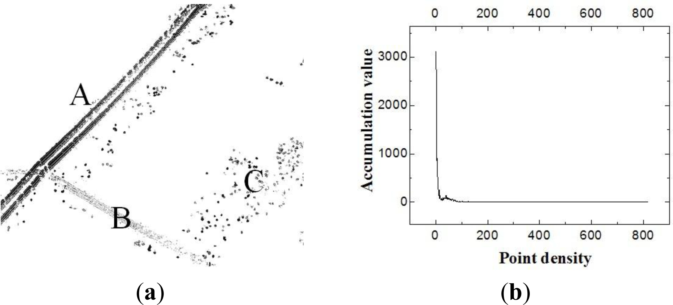
• Step 2: For all of the neighboring voxels, if the point density of a voxel is within the interval S_j, then increase the accumulation value Acc_j by 1, i.e., Acc_j = Acc_j + 1, thereby obtaining the point density accumulation chart, as shown in Figure 4b. In this figure, the peak interval corresponds to the non-power line points and the others correspond to the power line points for the following reasons: (1) In a grid there may be just few points, such as one or two points, in this case they may not be filtered using above single voxel filtering method; (2) Such situations are extremely common in the point cloud.
• Step 3: Based on the point density accumulation curve, calculate the partial derivative and find the peak interval. Eliminate the points inside the grids corresponding to the peak interval and the remained points are power line points.

(b) Hough transform. Hough transform is a technique used to find features of a particular shape by a voting procedure. This voting procedure is carried out in a parameter space, from which object candidates are obtained as local maxima in a so-called accumulator space. The power line points have a linear distribution on the O-XY plane so the Hough transform can be used to detect the power lines. Project the points onto the O-XY plane and use the equation p = xcosθ + ysinθ to map the coordinates to the parameter space (p, θ) where p/sinθ represents the intercept and −cosθ/sinθ represents the slope of the line. After that, extract the peak value to obtain the locations of the power line points. Create small buffers for these lines and use the points in the buffers to refer to the power line points. The width of the buffers is about two times the voxel size.

3.2. Power Line Points Clustering

The Hough transform can cluster the power line points in each line corridor on the O-XY plane. However, a structure such as Figure 5a may appear in the section of the line corridor. The power lines in this figure cross several spans and there are several power lines in each span. To fit each power line, the points A, B, C, and D should be clustered first, with the aim of identifying the points belonging to a single power line. Melzer and Briese [7] applied the RANSAC operation iteratively and clustered the points based on the distance between the points and a predicted model. This method depends greatly on the predictive model used. Liang et al. [11] considered that points in the same power line would be close together whereas the points in different power lines would be far apart. Therefore, a power line points clustering method based on KD trees was adopted. This method only considered the point distance and it ignored breakage points, which may have detrimental effects. Jwa and Sohn [14] proposed a piecewise catenary curve model-growing algorithm to identify the points, which achieved clustering by iterative catenary curve fitting and cubic growing. To a certain degree, this method is similar to the iterative RANSAC method, which is limited with the fitting curve and the selection of the initial growing cube. Related power line extraction methods focus little on the clustering of power line points.

The differences between vehicle-borne LiDAR and airborne LiDAR mean that power line points clustering is more difficult for vehicle-borne LiDAR. Vehicle-borne LiDAR points are more intensive and may be partially covered by trees and buildings, so the power line points have a dense-breakage-dense distribution pattern, as shown in Figure 5b. This problem needs to be addressed to cluster the vehicle-borne LiDAR points. Thus, we developed a bottom-up power line points clustering method based on initial clustering and cluster recovery.

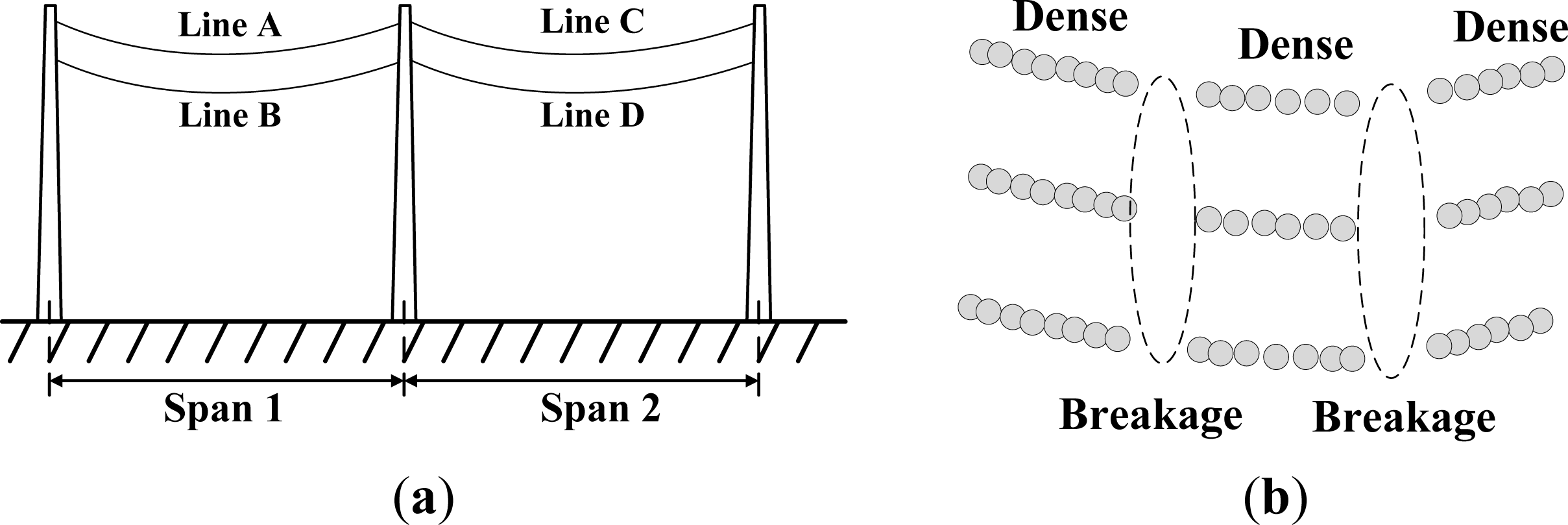
3.2.1. Initial Clustering

The power line points acquired by vehicle-borne LiDAR system exhibit a dense breakage-dense distribution pattern, so the intensively distributed points can be clustered initially based on their point distance. We used the AutoClust algorithm [32] for this purpose, which is a points clustering method with Delaunay triangulation. As for a Delaunay triangulation made of point set P, no point in P is inside the circumcircle of angle triangle in the Delaunay triangulation. Delaunay triangulations maximize the minimum angle of all the angles of the triangles in the triangulation. In Delaunay triangulation, the triangle is small and the edge length is short in areas with high point density point, and vice versa. The edge length of the triangles changes greatly as the density varies among areas. AutoClust performs triangulation based on this feature. For the points in Figure 5b, nine initial clusters can be obtained using the AutoClust algorithm.

The AutoClust algorithm can be used to cluster closely distributed points. However, breakage means that points belonging to a same power line can also be divided into different clusters, which means that other characteristics should be used for further clustering. There are four power lines in Figure 6a. The arrow lines are fitted lines based on local points (local fitted lines). In this figure, the angles and vertical distances of the neighboring local fitted lines of the same power lines are relatively small, such as A and B in power line 1. However, the vertical distances of the local fitted lines for different power lines such as A and C are relatively large, although their angles may be small. Based on this characteristic, it is easy to classify the power lines on the same span. It should be noted that for a local fitted line A, another local fitted line (like D) on different spans may also satisfy the angle and vertical distance conditions. In this case, the horizontal distance between the two local fitted lines should be taken into consideration and the line with an obvious large horizontal distance should be eliminated. Based on these considerations, we developed a cluster-growing method based on local straight line fitting.

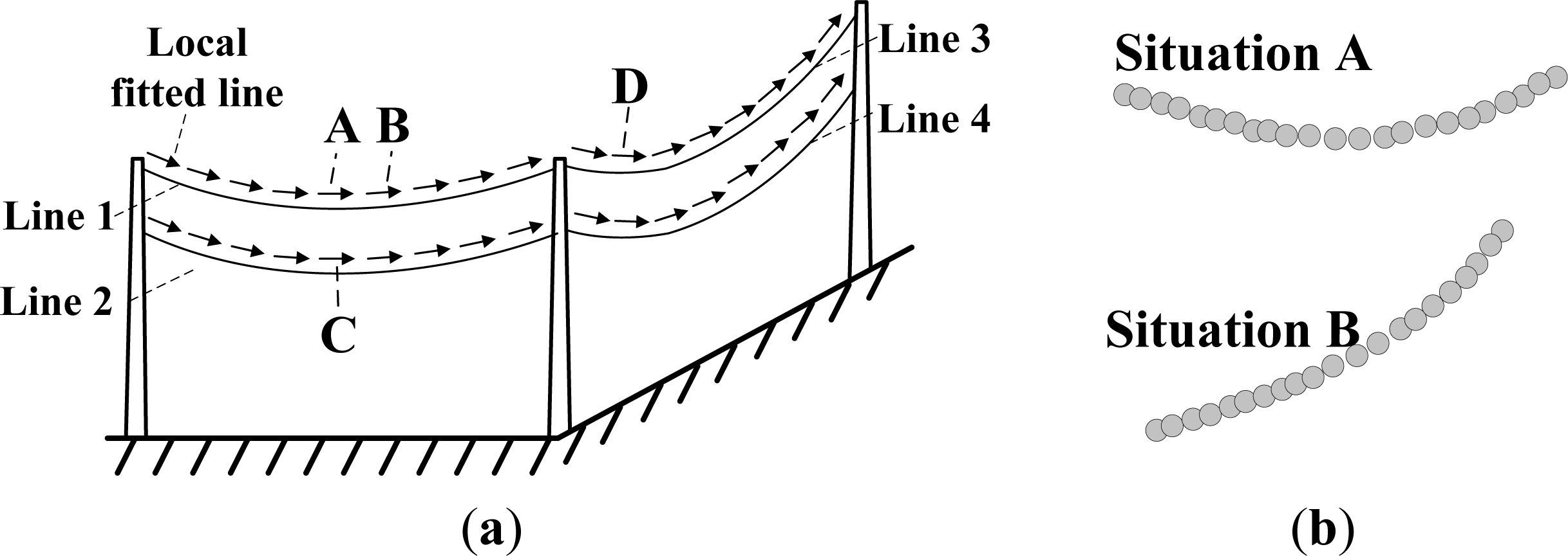
• Step 1: Generation of local fitted straight lines. If there are few points in the initial clusters, the fitting procedure may not be conducted. If the horizontal span of the cluster is large, cases such as those shown in Figure 6b may occur. If all of the points are used to fit the line directly, the fitted line cannot represent the actual distribution characteristics of the cluster. Thus, the initial clusters are divided into three types based on the number of points and the span width. If the number of points is less than a threshold (5), this cluster is not used to fit a line for the reason that large error may exist. If the span width is larger than a threshold (3 m), the points within certain limits (1 m) are used to fit the lines, which represent the extension directions of this cluster. The span width threshold and the limit threshold need to be set according to the sagging posture of power lines. The more obviously the power lines sag, the smaller the thresholds are. For other clusters, all of the points within them are used to fit the line.
• Step 2: Baseline for growing. Select any non-grown fitted line as the baseline and start the growing procedure.
• Step 3: Determination of the straight line that needs to be grown. Calculate the angle between the non-grown lines and the baseline. If the angle is smaller than a certain threshold (10°), rotate the baseline until it is parallel with the fitted line and calculate the vertical distance between the two lines. If the distance is smaller than a threshold (0.2 m), this fitted line is marked as the line to be grown. Here, the angle threshold is set according to the sagging posture of power lines. The more obviously the power lines sag, the larger the angle threshold is. The distance threshold should be set smaller than the distance of up-down power lines.
• Step 4: Growing fitted local straight lines. Merge the points in the current baseline and the line to be grown into one cluster and set the line to be grown as the new baseline. During the growing process, calculate the average vertical distance between the cluster without a local fitted line (filters with few points) and the current baseline. If the distance is less than the lower threshold (0.1 m), merge them. Repeat Steps 2–4 until all of the local fitted lines have completed their growing procedures.

3.2.2. Cluster Recovery

The growing method with local fitted lines can cluster points belonging to the same power line. However, this method is based on straight lines whereas power lines are curves in practice. If the power line curvature is high and there is too much occlusion, the angles and vertical distances of the adjacent local fitted lines on the same power line can also be very high, as shown by lines A and B, and C and D in Figure 7a. As a result, the base of the local fitted line grows, so we developed a cluster recovery method to cope with these extreme conditions. The specific procedures are as follows.

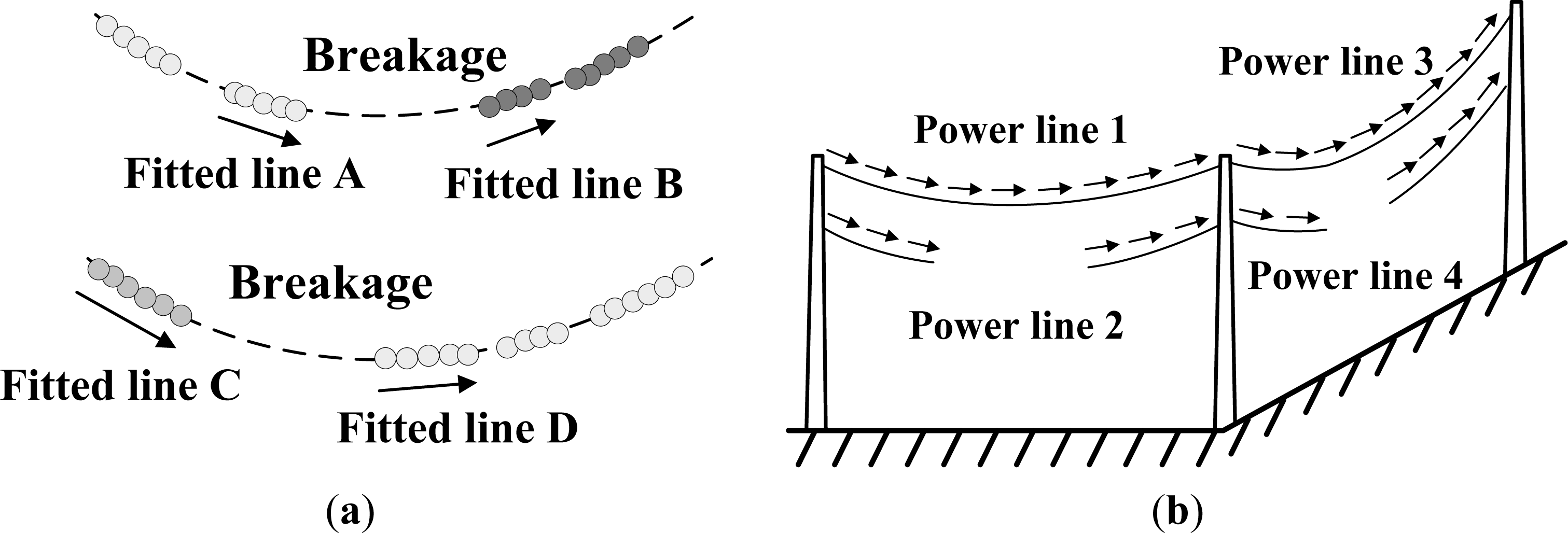
• Step 1: Identification of broken clusters. After completing the clustering of a single power line, the local fitted lines will exhibit a trend like the arrows shown on power lines 1 and 3 in Figure 7b, whereas clusters with breakage will resemble power lines 2 and 4. As for power lines 2, the two fitted local lines of the left line both lie within [−90°, 0°] with those of right line within [0°, 90°]. The same situation appears for power line 4. The broken clusters can be identified based on these characteristics. The local lines (span width 3 m) are fitted on the right and left side of each cluster and if the angles of these two fitted local lines lie within [−90°, 0°] or [0°, 90°], the cluster is a broken cluster. Here the span width threshold needs to be set according to the sagging posture of power lines. The more obviously the power lines sag, the smaller the threshold is.
• Step 2: Recovery of broken clusters. For the current broken cluster, select another broken cluster within the span width. Use the least squares algorithm to fit a parabola to the points in the current broken cluster and other broken clusters, and record the residual. Merge the broken clusters based on the smallest residual and calculate the distance between this fitted model and other broken clusters. If the average distance is less than a threshold (0.1 m), merge them.
• Step 3: Repeat Step 2 for all broken clusters, thereby completing the cluster recovery procedure.

3.3. 3D Power Line Fitting

After clustering the single power line points, mathematical models can be used to fit the power lines. Based on the characteristics of two high ends and the low middle, which is similar to a parabola, we used the polynomial equation z = ax² + bxy + cy² + d to fit the power lines. Figure 8a shows the power line points and Figure 8b shows the fitted power line. We can see that the fitted curve agrees with the power line points. Thus, it is reasonable to use this polynomial equation to fit the power lines.

3.4. Sensitivity Analysis on the Key Parameters

As a few parameters are set in this method, a summarization on the setting of the key parameters is necessary. The setting basis of these thresholds includes three types: calculation, data source, and empiric. The term “calculation” indicates that the threshold can be calculated automatically in the method. As for the term “data source”, it means that the thresholds are set according to the real data. If this method is applied in some other areas for extraction of urban power lines, the “calculation” and “data source” thresholds are easy to be determined automatically, which cannot limit the applicability of the proposed method. The term “empiric” means that the thresholds are set empirically and in most cases they can be set as we proposed here directly.

During the extraction of power line points, a voxel-based hierarchical method is introduced. In this method, single voxel filtering and neighboring voxel filtering is conducted respectively. The parameters during these two steps are shown in

Table 1. Key parameters in the method.

		Threshold	Scale	Setting Basis
Power line points extraction	Single voxel filtering	Voxel size	[10 cm, distpl]	Data source
		Ground points	1 m	Empiric
		Terrain clearance	2 m	Empiric
		Up-down continuity	3	Data source
		Feature eigenvector	0.3	Empiric
	Neighboring voxel filtering	Voxel size	3 × 3 × 3 or 5 × 5 × 5	Empiric
		Point density	Automatic	Calculation
Power line points clustering	Initial clustering	Point number of local fitted lines	5	Empiric
		Span width of local fitted lines	3 m	Data source
		Angle of to-be grown lines	10 g	Data source
		Distance of to-be grown lines	0.2 m	Empiric
	Cluster recovery	Span width of broken clusters	3 m	Data source
		Distance of to-be merged clusters	0.1 m	Empiric

. In the table, several parameters are presented. Here, the size of a single voxel and up-down continuity needs to be set according to the data source. As for the size of a single voxel, elaborative consideration has been given at the end of Section 3.1.1 and it is set to [10 cm, dist_pl], where dist_pl is the minimum distance between different power lines and 10 cm is set empirically. As for the threshold of up-down continuity, it needs to be set according to the real data source. In some cases, the power lines are closely near ground objects or other power lines, then the threshold should be small, otherwise it can be set a little larger.

During power line points clustering, a bottom-up power line points clustering method based on initial clustering, cluster growing and cluster recovery is used. The key parameters are shown in the table. As we can see, the point number of local fitted lines, distance of to-be grown lines and distance of to-be merged clusters can be set empirically. The other thresholds need to be set according to the real data source. Here, the key factor to be considered is the sagging posture of the real power lines. The more obviously the power lines sag, the smaller the thresholds are.

4. Experiments

The algorithm proposed was programmed in C# on Microsoft Visual Studio platform. The hardware system was a computer with 3 GB of RAM and a dual-core 3 GHz processor.

4.1. Power Line Points Extraction

Figure 9 shows the procedures used to extract the power line points from the vehicle-borne LiDAR data. In Figure 9a, 3-D voxels of 0.4 × 0.4 × 0.4 m² were constructed and filtered using an elevation difference of 1 m. We obtained 6,813,103 non-ground points. Figure 9b shows the filtering results for the non-ground points with a terrain clearance of 2 m. In this figure, only the points of power lines, trees, streetlights, and buildings remain, and the total number of points was 3,919,815. In Figure 9c, up-down continuity filtering eliminated many points related to the woods, streetlights, and buildings so 111,782 points remained. In Figure 9d, the feature eigenvectors were calculated for the points in each voxel and the linearity threshold was set to 0.3. After filtering, many points that corresponded to trees were eliminated, which only left some discrete points related to woods. For the neighboring voxel filtering method, the window size was set as 5 × 5 × 5 and the point density threshold was calculated automatically as 15. The results are shown in Figure 9e. Finally, the Hough transform was applied to the filtering shown in Figure 9f, where most of the remaining points were power line points. The extraction of power line points costs about 82 s.

To evaluate the extracted power line points quantitatively, power lines are digitized from the original points and extracted power line points, respectively. The lengths of extracted power lines were used as the evaluation objects. Here, the number of power line points is not fit for the evaluation, because point density may vary and in some situations despite many power line points being extracted, they may gather together and could not reflect the real distribution of power lines. The correctness and completeness were used as indexes for evaluation, as follows:

$$\begin{array}{l}\mathit{Completeness}=\frac{\mathit{TP}}{\mathit{TP}+\mathit{FN}}\\ \mathit{Correctness}=\frac{\mathit{TP}}{\mathit{TP}+\mathit{FP}}\end{array}$$

where True Positive (TP) refers to the length of correctly extracted power line points, False Negative (FN) is the length of missing power lines, and False Positive (FP) is the length of extracted incorrect power lines.

As shown in

Table 2. Correctness and completeness of the extracted power line points.

	Actual Length	Correct Length	Incorrect Length	Missing Length	Correctness	Completeness
Result	4006	3764	36	242	99.1%	93.9%

, the length of real power lines was 4006 m while the length of extracted power lines was 3800 m. We found that TP, FN, and FP were 3764 m, 242 m, and 36 m, respectively. Thus, the correctness and completeness of the extracted power lines were 99.1% and 93.9%, respectively. This showed that the power line points extraction methods from vehicle-borne LiDAR data delivered good results with high correctness and completeness.

4.2. Power Line Points Clustering

Figure 10 shows the power line points clustered using the proposed method. The AutoClust algorithm was used in Figure 10a for the initial filtering and 94 clusters were obtained. Next, local fitted lines were generated and grown, and three clusters remained in Figure 10b. The figure shows that the points belonging to the three power lines were all divided effectively. Figure 10c shows the clustering results for the overall dataset where 105 clusters were obtained. Figure 10d shows magnified images of A and B in Figure 10c. This procedure costs about 15 s.

We clustered all of the power line points manually and compared them with the results obtained using our proposed method. A cluster was considered to be complete if the clustering results for the points on a specific power line corresponded to the actual clusters (over 90% of the points were clustered successfully). If points from several power lines were clustered into one cluster, this was considered to be over-clustering. If the points on one power line were divided into two or more clusters, this was considered inadequate clustering. If a specific cluster was missed, this was treated as a missing cluster.

Table 3. Evaluation of the clustering of power line points.

	Actual Cluster	Complete Cluster	Over-Clustered	Inadequate Cluster	Missing Cluster
Number	105	102	0	3	0
Rate	100%	97.2%	0	2.8%	0

shows the evaluation results for the clustering of the power line points. There were 105 power lines, which corresponded to 105 clusters. Using the proposed method, we obtained 102 complete clusters, three incomplete clusters, and no over-clustered or missed clusters.

4.3. Three-Dimensional Power Line Fitting

The polynomial model was used to fit the points of the 102 complete power lines and the results obtained are shown in Figure 11. Figure 11a shows that all of the power lines were fitted effectively and the result represented the actual distributions of the power lines. Figure 11b shows magnified sections of the fitted results, which correspond to A, B, C, and D in Figure 11a. Each magnified section shows that the points corresponded to the fitted curve correctly.

To evaluate the accuracy of the fitted results quantitatively, we calculated the distances between all of the power line points and their corresponding fitted curves.

Table 4. Evaluation of the fitted three-dimensional power lines.

	Average (cm)	Maximum (cm)	RMSE (cm)
Distance	2.1	6.7	2.4

shows that the average distance between the points and the fitted curves was 2.1 cm, with a maximum of 6.7 cm and the RMSE was 2.4 cm. The overall error of the fitted power lines using the proposed method was about 2 cm, which demonstrated the relatively high accuracy of the method.

5. Conclusions

In this study, a complete work-flow for extracting urban power lines from vehicle-borne LiDAR data is developed, which comprises the extraction of power line points, single power line points clustering, and 3-D power line fitting. First, a voxel-based hierarchical method is developed to extract the power line points. The terrain clearance, up-down continuity, and feature eigenvectors are used initially for single voxel filtering. Next, the point densities of neighboring voxels are calculated for further filtering. A point density accumulation method is proposed for the determination of point density threshold. On this basis, a bottom-up power line points clustering method is introduced to identify the points belonging to a single power line. AutoClust is used for the initial clustering, and local fitted lines and then local fitted lines are utilized for growing and recovering the initial clusters. The experiment shows that the proposed methods could extract power line points from vehicle-borne LiDAR points effectively. The correctness and completeness of the extracted points are relatively high. The power line points clustering method can cluster the points with a high level of correctness. Using the proposed technique, power lines can be extracted automatically with a high degree of accuracy. Nevertheless, there are also some limitations of this technique. The main limitation lies in the setting of thresholds, especially in the clustering of power line points. During the generation of local fitted lines, the initial clusters are divided into three types where span width and limit thresholds are used. These two thresholds need to be set according to the sagging posture of power lines, which calls for experience. The same situation occurs in the growing of local fitted lines. Another limitation lies in the absence of telegraph poles and pylons, which are also important assets for power line patrols. Future work will be oriented to these limitations. On one hand, a more automatic power line clustering method is to be studied. On the other hand, the telegraph pole and pylons will be reconstructed.

References

1. Ussyshkin, R.V.; Theriault, L.; Sitar, M.; Kou, T. Advantages of Airborne Lidar Technology in Power Line Asset Management. Proceedings of the 2011 International Workshop on Multi-Platform/Multi-Sensor Remote Sensing and Mapping (M2RSM), Xiamen, China, 10–12 January 2011; pp. 1–5.
2. Lu, M.L.; Pfrimmer, G.; Kieloch, Z. Upgrading an Existing 138 kV Transmission Line in Manitoba. Proceedings of 2006 IEEE Power Engineering Society General Meeting, Montreal, QC, Canada, 18–22 June 2006; pp. 964–970.
3. Koop, J.E. Advanced technology for transmission line modeling. Transm. Distrib. World 2002, 54, 90–93. [Google Scholar]
4. Ashidate, S.; Murashima, S.; Fujii, N. Development of a helicopter-mounted eye-safe laser radar system for distance measurement between power transmission lines and nearby trees. IEEE Trans. Power Deliv 2002, 17, 644–648. [Google Scholar]
5. Filin, S.; Pfeifer, N. Segmentation of airborne laser scanning data using a slope adaptive neighborhood. ISPRS J. Photogramm. Remote Sens 2006, 60, 71–80. [Google Scholar]
6. Jahromi, A.B.; Zoej, M.J.V.; Mohammadzadeh, A.; Sadeghian, S. A novel filtering algorithm for bare-earth extraction from airborne laser scanning data using an artificial neural network. IEEE J. Sel. Top. Appl. Earth Obs. Remote Sens 2011, 4, 836–843. [Google Scholar]
7. Melzer, T.; Briese, C. Extraction and Modeling of Power Lines from ALS Point Clouds. Proceedings of the 28th Workshop of the Austrian Association for pattern Recognition, Hagenberg, Austria, 17–18 June 2004; pp. 47–54.
8. McLaughlin, R.A. Extracting transmission lines from airborne LiDAR data. IEEE Geosci. Remote Sens. Lett 2006, 3, 222–226. [Google Scholar]
9. Liu, Y.; Li, Z.; Hayward, R.; Walker, R.; Jin, H. Classification of Airborne Lidar Intensity Data Using Statistical Analysis and Hough Transform with Application to Power Line Corridors. Proceedings of the 2009 Digital Image Computing: Techniques and Applications, Melbourne, Australia, 1–3 December 2009; pp. 462–467.
10. Yu, J.; Mu, C.; Feng, Y.; Dou, Y. Powerlines extraction techniques from airborne LiDAR data. Geomat. Inf. Sci. Wuhan Univ 2011, 36, 1275–1279. (In Chinese) [Google Scholar]
11. Liang, J.; Zhang, J.; Liu, Z. On extracting power-line from airborne LiDAR point cloud data. Bull. Surv. Mapp 2012, 7, 17–20. (In Chinese) [Google Scholar]
12. Jwa, Y.; Sohn, G.; Kim, H.B. Automatic 3D powerline reconstruction using airborne lidar data. Int. Arch. Photogramm. Remote Sens 2009, 38, 105–110. [Google Scholar]
13. Jwa, Y.; Sohn, G. A piecewise catenary curve model growing for 3D power line reconstruction. Photogramm. Eng. Remote Sens 2012, 78, 1227–1240. [Google Scholar]
14. Ackermann, F. Airborne laser scanning-present status and future expectations. ISPRS J. Photogramm. Remote Sens 1999, 54, 64–67. [Google Scholar]
15. Baltsavias, E.P. Airborne laser scanning: Existing systems and firms and other resources. ISPRS J. Photogramm. Remote Sens 1999, 54, 164–198. [Google Scholar]
16. Jwa, Y.; Sohn, G. A multi-level span analysis for improving 3D power-line reconstruction performance using airborne laser scanning data. Int. Arch. Photogramm. Remote Sens. Spat. Inf. Sci 2010, 38, 97–102. [Google Scholar]
17. Zhang, X.; Chen, G.; Long, W.; Cheng, Z.; Zhang, K. Current status and prospects of helicopter power line inspection tour with LiDAR. Electr. Power Constr 2008, 29, 40–43. [Google Scholar]
18. Ou, T.; Geng, X.; Yang, B. Application of vehicle-borne data acquisition system to power line detection. J. Geod. Geodyn 2009, 29, 149–151. [Google Scholar]
19. Abdallah, H.; Bailly, J.; Baghdadi, N.N.; Saint-Geours, N.; Fabre, F. Potential of space-borne LiDAR sensors for global bathymetry in coastal and inland waters. IEEE J. Sel. Top. Appl. Earth Obs. Remote Sens 2013, 6, 202–216. [Google Scholar]
20. Lehtomäki, M.; Jaakkola, A.; Hyyppä, J.; Kukko, A.; Kaartinen, H. Detection of vertical pole-like objects in a road environment using vehicle-based laser scanning data. Remote Sens 2010, 2, 641–664. [Google Scholar]
21. Wu, B.; Yu, B.; Yue, W.; Shu, S.; Tan, W.; Hu, C.; Huang, Y.; Wu, J.; Liu, H.X. A voxel-based method for automated identification and morphological parameters estimation of individual street trees from mobile laser scanning data. Remote Sens 2013, 5, 584–611. [Google Scholar]
22. Wu, B.; Yu, B.; Yue, W.; Wu, J.; Huang, Y. Voxel-Based Marked Neighborhood Searching Method for Identifying Street Trees Using Vehicle-Borne Laser Scanning Data. Proceedings of the Second International Workshop on Earth Observation and Remote Sensing Applications (EORSA), Shanghai, China, 8–11 June 2012; pp. 327–331.
23. Jaakkola, A.; Hyyppä, J.; Hyyppä, H.; Kukko, A. Retrieval algorithms for road surface modelling using laser-based mobile mapping. Sensors 2008, 8, 5238–5249. [Google Scholar]
24. Zhu, L.; Hyyppä, J.; Kukko, A.; Kaartinen, H.; Chen, R. Photorealistic building reconstruction from mobile laser scanning data. Remote Sens 2011, 3, 1406–1426. [Google Scholar]
25. Jaakkola, A.; Hyyppä, J.; Kukko, A.; Yu, X.; Kaartinen, H.; Lehtomäki, M.; Lin, Y. A low-cost multi-sensoral mobile mapping system and its feasibility for tree measurements. ISPRS J. Photogramm. Remote Sens 2010, 65, 514–522. [Google Scholar]
26. Hu, Y.; Li, X.; Xie, J.; Guo, L. A. Novel Approach to Extracting Street Lamps from Vehicle-Borne Laser Data. Proceedings of the 19th International Conference on Geoinformatics, Shanghai, China, 24–26 June 2011; pp. 1–6.
27. Lam, J.; Kusevic, K.; Mrstikl, P.; Harrap, R.; Greenspan, M. Urban Scene Extraction from Mobile Ground Based LiDAR Data. Proceedings of the 5th International Symposium on 3D Data Processing, Visualisation and Transmission, Paris, France, 17–20 May 2010; pp. 1–8.
28. Biosca, J.M.; Lerma, J.L. Unsupervised robust planar segmentation of terrestrial laser scanner point clouds based on fuzzy clustering methods. ISPRS J. Photogramm. Remote Sens 2008, 63, 84–98. [Google Scholar]
29. Yang, B.; Wei, Z.; Li, Q.; Li, J. Automated extraction of street-scene objects from mobile lidar point clouds. Int. J. Remote Sens 2012, 33, 5839–5861. [Google Scholar]
30. Aijazi, A.K.; Checchin, P.; Trassoudaine, L. Segmentation based classification of 3D urban point clouds: A super-voxel based approach with evaluation. Remote Sens 2013, 5, 1624–1650. [Google Scholar]
31. Kim, H.B.; Sohn, G. 3D classification of power-line scene from airborne laser scanning data using random forests. Int. Arch. Photogramm. Remote Sens 2010, 38, 126–132. [Google Scholar]
32. Estivill-Castro, V.; Lee, I. Argument free clustering for large spatial point-data sets via boundary extraction from Delaunay diagram. Comput. Environ. Urban Syst 2002, 26, 315–334. [Google Scholar]
Figure 1. Example of a multiple parallel power line structure.
Remotesensing 06 03302f1
Figure 2. Experimental data. (a) Vehicle-borne LiDAR points. (b) Experimental area.
Remotesensing 06 03302f2
Figure 3. Flow of the power line extraction procedure based on vehicle-borne LiDAR data.
Remotesensing 06 03302f3
Figure 4. Neighboring voxel filtering. (a) A single voxel filtering example. (b) Point density accumulation.
Remotesensing 06 03302f4
Figure 5. Clustering of power line points. (a) Section of a power line corridor. (b) Power line points in vehicle-borne LiDAR data.
Remotesensing 06 03302f5
Figure 6. Cluster growing with local fitted straight lines. (a) Example showing local fitted lines. (b) An example of a cluster with a large span.
Remotesensing 06 03302f6
Figure 7. Cluster recovery. (a) High curvature with large occlusions. (b) Identification of broken clusters.
Remotesensing 06 03302f7
Figure 8. Three-dimensional power line fitting. (a) Power line points. (b) Fitted curve.
Remotesensing 06 03302f8
Figure 9. Power line extraction procedures. (a) Ground truth points filtering. (b) Terrain clearance filtering. (c) Up-down continuity filtering. (d) Feature eigenvector filtering. (e) Point density filtering. (f) Hough transform filtering.
Remotesensing 06 03302f9
Figure 10. Power line points clustering. (a) Clustering results using AutoClust. (b) Growing the local fitted lines. (c) Clustering results for the overall dataset. (d) Magnified sections of clustered result at points A and B.
Remotesensing 06 03302f10
Figure 11. Three-dimensional (3-D) power line fitting. (a) The fitted 3-D power lines. (b) Magnified sections of the fitted result at points A, B, C and D.
Remotesensing 06 03302f11