Evaluating Parameter Adjustment in the MODIS Gross Primary Production Algorithm Based on Eddy Covariance Tower Measurements

Abstract

How well parameterization will improve gross primary production (GPP) estimation using the MODerate-resolution Imaging Spectroradiometer (MODIS) algorithm has been rarely investigated. We adjusted the parameters in the algorithm for 21 selected eddy-covariance flux towers which represented nine typical plant functional types (PFTs). We then compared these estimates of the MOD17A2 product, by the MODIS algorithm with default parameters in the Biome Property Look-Up Table, and by a two-leaf Farquhar model. The results indicate that optimizing the maximum light use efficiency (ɛ_max) in the algorithm would improve GPP estimation, especially for deciduous vegetation, though it could not compensate the underestimation during summer caused by the one-leaf upscaling strategy. Adding the soil water factor to the algorithm would not significantly affect performance, but it could make the adjusted ɛ_max more robust for sites with the same PFT and among different PFTs. Even with adjusted parameters, both one-leaf and two-leaf models would not capture seasonally photosynthetic dynamics, thereby we suggest that further improvement in GPP estimaiton is required by taking into consideration seasonal variations of the key parameters and variables.

1. Introduction

Gross primary production (GPP), which is the amount of light energy from the sun converted to chemical energy, determines the thermal, water and biogeochemical cycles in terrestrial ecosystems. However, even when eddy covariance (EC) flux data and remote sensing data are conjunctively introduced into various diagnostic models, uncertainties in modeled GPP are still vast. Current estimates of global GPP range between 102 and 165 petagrams of carbon per year, where uncertainties are likely from errors of input data, poor parameterization and model structure [1–6]. Among the methods of reducing uncertainties in GPP simulation, parameter adjustment and structural modification are adopted, and the former method could compensate for the errors introduced by a model structure [2,7,8].

Many concepts were developed to simulate carbon assimilation [9–11]. One of the widely accepted approaches is the light use efficiency model because of both its simple structure—which assumes that a fraction of the photosynthetically active radiation (PAR) absorbed by the vegetation canopy is used for plant primary production [9]—and its large amount of available input data, including EC measurements [12–15] and remotely sensed data [16–18]. One application of this kind of model is the MODIS GPP algorithm [19]. Its latest product MOD17A2 Collection 5 ( https://lpdaac.usgs.gov/products) is forced by the National Center for Environmental Prediction–Department of Energy (NCEP-DOE) reanalysis II data and the default parameters are derived from the Biome Property Look-Up Table (BPLUT) [20].

Based on the algorithm and its product, many evaluations have been made. Early studies focused on uncertainties introduced by input data [5,16,21] and simulations using different input data [17,22,23]. A direct comparison between the NCEP-DOC reanalysis II data and EC tower measurements at 12 African sites suggested that these two forcing data with different spatial resolutions were comparable in air temperature and atmospheric vapor pressure deficit (VPD), but the relationship was scattered in incoming PAR [14]. Recently, many studies paid attention to structural errors of the MODIS GPP algorithm. Zhang et al. [24] compared the MODIS GPP product with the estimates using a process-based ecosystem model (Boreal Ecosystem Productivity Simulator). They noted that the MODIS GPP algorithm cannot properly treat the contribution of shaded leaves to canopy-level GPP. He et al. [13,15] developed a two-leaf light use efficiency model for improving the calculation of GPP and validated its application in six ecosystems. Previously, the two-leaf upscaling strategy had been well documented in the Farquhar model, as compared with the one-leaf strategy [25,26]. Aside from model restructure, adjusting biome parameters is another way to improve simulation. Evaluations of MODIS GPP using EC data indicated that adjusting the maximum light use efficiency (ɛ_max), which was derived from the BPLUT [19,20], in the algorithm might be needed to better estimate GPP in both Africa [14] and northern China [27]. As a key parameter in the algorithm, ɛ_max was further affected by the scales of daily minimum temperature (T_MIN) and VPD [19]. However, the T_MIN function was observed not to constrain MOD17A2 GPP much [8,14] and both functions could be corrected using flux tower measurements [8]. Moreover, some studies noted that optimizing the algorithm using the soil water content can improve agreement with the measurements [28], but only in dry regions [14,29,30] or throughout the growing season [16].

As mentioned above, both adjusting the key parameters and modifying the model structure can improve GPP estimation using the MODIS algorithm, and the former can compensate for errors introduced by the latter [2,7,8]. Therefore, the best approach for improving the algorithm is open to debate, and benefits of parameter adjustment are needed to be validated for multiple biome types across different time scales and over relatively long time periods. Furthermore, less attention has been given to the effects of adopting different methods of parameter adjustment, such as using model–data fusion [31] and adding control factors [2]. These issues must be clarified and resolved to reduce uncertainties in GPP estimates on regional and global scales.

We hypothesize that adjusting key parameter can improve estimates and can compensate for structural errors caused by adopting the one-leaf strategy in the MODIS GPP algorithm. The objective of this study is to evaluate capacity of parameter adjustment in the algorithm to improve estimates for multiple plant functional types. We used EC measurements to optimize key parameters in the algorithm. The selected EC towers represented nine plant functional types across six biomes in two main climate zones. Then we compared the adjusted models with the MOD17A2, the algorithm with default parameters, and a two-leaf Farquhar model across half hourly, daily, monthly and seasonal time scales. The Farquhar model is a default component of the Dynamic Land Model (DLM) [32,33]. By using an existing dataset, this research proves a solid foundation for evaluating the MODIS algorithm’s ability to estimate GPP across multiple plant functional types and a range of time scales.

2. Materials and Methods

2.1. Data

2.1.1. Eddy-Covariance Data

We used the FLUXNET database ( http://fluxnet.ornl.gov/) to calibrate the models and to validate GPP estimates. The dataset contains annual files of half-hourly meteorological and flux data from more than 400 EC sites across Europe (CarboEurope), America (AmeriFlux and Fluxnet-Canada), and Asia (AisaFlux and ChinaFLUX), etc. To reduce potential errors derived from the observations, we selected the EC towers according to the following criteria: (1) the site provides four or more years of continuous data as a part of the publicly accessible standardized Level 4 or 3 database; (2) a “site-year” is accepted for analysis if more than 90% of the half hours in a year contain non-missing values for the meteorological data (downwelling solar radiation, precipitation, wind speed, air temperature and relative humidity), the carbon flux data (net ecosystem exchange and ecosystem respiration (R_eco)), and the energy fluxes (net radiation (R_n), ground heat flux (G), latent heat flux (LE) and sensible heat flux (H)); and (3) energy balance closure is evaluated for each site-year according to the ratio of the dependent flux variables (H + LE) against the independently derived available energy (R_n − G) for each half hour [34]. The values of the half-hourly energy balance closure ratio (H + LE)/(R_n − G) deviate from the ideal closure (a value of 1) because random error exists, and the magnitude of the CO₂ uptake is less when the energy imbalance is greater [34,35]. Thus we recorded the number of daytime half hours of which the ratio was in the range of 0.6–1.4, and then accepted a “site-year” when the accumulated number was greater than 60% of the total number of daytime half hours during the growing season. Uncertainties in the EC-measured GPP still exist because of the underestimation of R_eco at night, gap filling algorithm uncertainty, partitioning uncertainty, random uncertainty, and threshold friction velocity uncertainty [36]. We considered the supplied GPP as the “ground truth” [18] in this study.

Finally, 102 site-years, which represent six biome types across two main climatic environment zones (i.e., plant functional types, PFTs) [37] at 21 EC sites [38–64], were selected (

Table 1. Descriptions of the study sites.

Number	Site ID a	Latitude (°N)	Longitude (°E)	Elevation (m)	Biome Type b	Climate Zone	Site-Years	Precipitation (mm·yr−1)	LAImax (m2·m−2)	References
1	CA-Ca1	49.867	−125.334	313	NEF	Temperate	2001–08(06) c	1456	7.3	Chen et al. (2011), Krishnan et al. (2009) [38,39]
2	CA-Ca2	49.871	−125.291	170	NEF	Temperate	2007–10(08)	619	2.7	Grant et al. (2010) [40]
3	CA-Ca3	49.535	−124.900	153	NEF	Temperate	2003–07(05)	1683	7.0	Grant et al. (2010) [40]
4	DE-Tha	50.964	13.567	380	NEF	Temperate	2001–05(01)	804	7.6	Grünwald and Bernhofer (2007) [41]
5	ES-ES1	39.346	−0.319	1	NEF	Mediterranean	2004–07(05)	414	2.6	Blyth et al. (2010) [42]
6	US-Ho1	45.204	−68.740	72	NEF	Temperate	1996–98, 2003–04(03)	951	5.7	Hollinger et al. (2004) [43]
7	CN-Qia	26.741	115.058	86	NEF	Temperate	2003–04, 2006–07(04)	1325	4.7	Li et al. (2007) [44]
8	CA-Ojp	53.916	−104.692	518	NEF	Boreal	2007–10(08)	418	2.0	Bergeron et al. (2007), Kljun et al. (2006) [45,46]
9	CA-Obs	53.987	−105.118	598	NEF	Boreal	2001–05(01)	408	3.4	Gaumont-Guay et al. (2014) [47]
10	CA-NS1	55.879	−98.484	253	NDF	Boreal	2002–06(03)	213	3.0c	Hill et al. (2011) [48]
11	FI-Hyy	61.847	24.295	185	NDF	Boreal	2005–08(06)	500	6.7	Tanja et al. (2003) [49]
12	FR-Pue	43.741	3.596	270	BEF	Mediterranean	2004–09(08)	1116	2.9	Rambal et al. (2003) [50]
13	IT-Cpz	41.705	12.376	9	BEF	Mediterranean	2006–09(07)	593	3.5	Garbulsky et al .(2008), Reichstein et al. (2007) [51,52]
14	IT-Col	41.849	13.588	1645	BDF	Mediterranean	2004–07(05)	954	6.4	Valentini et al. (1996) [53]
15	US-MOz	38.744	−92.200	212	BDF	Mediterranean	2004–08(05)	1023	4.0	Gu et al. (2006) [54]
16	CA-Oas	53.629	−106.198	580	BDF	Boreal	2001–05(03)	261	2.6	Barr et al. (2007), Krishnan et al. (2006) [55,56]
17	DK-Sor	55.487	11.646	40	BDF	Boreal	2003–05, 2008–09(04)	631	5.0	Pilegaard et al. (2003) [57]
18	CA-Mer	45.409	−75.519	65	BDS	Temperate	2004–07(06)	1203	1.2	Lafleur et al. (2003), Roulet et al. (2007) [58,59]
19	CA-NS6	55.917	−98.964	271	BDS	Boreal	2002–06(02)	267	3.0 d	Goulden et al. (2006), McMillan et al. (2008) [60,61]
20	AT-Neu	47.116	11.320	970	GRA	Temperate	2002–07(03)	764	6.5	Wohlfahrt et al. (2008) [62]
21	IE-Dri	51.987	−8.752	187	GRA	Temperate	2002–06(04)	1341	5.2 c	Montaldo et al. (2007), Peichl et al. (2010) [63,64]

Note:

^aThe site ID is taken from FLUXNET.

^bBiome types: needleleaf evergreen forest (NEF), needleleaf deciduous forest (NDF), broadleaf evergreen forest (BEF), broadleaf deciduous forest (BDF), broadleaf deciduous shrub (BDS), and grassland (GRA).

^cThe selected years of each site. The number in parentheses is the representative year for analyzing.

^dData were extracted from a global LAI map based on 10-day synthesis VEGETATION images at 1-km spatial resolution [4,76,77].

). Seven of these sites are in boreal regions, and fourteen sites are in temperate regions. Five sites that have Mediterranean climates were characterized as being in the temperate zone because of the absence of Mediterranean forest in the PFTs we used [37]. Though the three sites, CA-Ca1, CA-Ca2 and CA-Ca3, were located in adjacent areas, their planting years were 1949, 2000 and 1988, respectively, indicating different tree ages. This is a similar case with CA-Ojp and CA-Obs; their planting years were 1929 and 1879, respectively. We used two years of each site for model calibration, and another two consecutive years for validation.

2.1.2. MODIS 8-Day Average GPP Product

The MODIS GPP product MOD17A2 Collection 5 was designed to provide an 8-day average measure of the global terrestrial vegetation using MODIS land cover, vegetation product and surface meteorology at 1 km resolution [20,65]. We used mean values of the 3-by-3 pixels, with the center pixel containing the tower location (Table 1). Because the footprint radius of most annual cumulative climatology data ranged from 0.70 to 1.5 km [66], the 3-by-3 pixel area is expected to represent the flux tower footprint well [18,67,68].

2.2. Model Description

2.2.1. MODIS GPP Algorithm

MOD17A2 is calculated using a light use efficiency model with the one-leaf upscaling strategy based on the radiation conversion efficiency concept of Monteith [9] as follows [19,20,69]:

$$\mathit{GPP}={\varepsilon }_{\mathit{max}}\times f(\mathit{VPD})\times f(T_{\mathit{air}})\times \mathit{PAR}\times \mathit{fPAR}$$

(1)

where PAR is the incident photosynthetically active radiation—its value is assumed to be 45% of the incident shortwave radiation [19]; ɛ_max is the maximum light use efficiency, which depends on the plant functional types; f(VPD) and f(T_air) are the scalars of vapor pressure deficit and air temperature, respectively, both of which are ranged from 0 to 1 to downscale the maximum light use efficiency of the canopy to the actual value. The scales were calculated as follows [8,13,15]:

$$f(\mathit{VPD})=\frac{{\mathit{VPD}}_{\mathit{max}}-\mathit{VPD}}{{\mathit{VPD}}_{\mathit{max}}-{\mathit{VPD}}_{\mathit{min}}}$$

(2)

$$f(T_{\mathit{air}})=\frac{T_{\mathit{air}}-T_{\mathit{MINmin}}}{T_{\mathit{MINmax}}-T_{\mathit{MINmin}}}$$

(3)

where VPD_max and T_MINmin are daily maximum VPD and daily minimum temperature at which the light use efficiency equals 0, and VPD_min and T_MINmax are daily minimum VPD and daily minimum temperature at which the light use efficiency is maximum. We replaced the daily minimum temperature in the temperature function [8,13,15] by EC-observed half-hourly temperature (T_air) to calculate GPP on half-hourly time scale. fPAR is the fraction of PAR being absorbed by the canopy, which was estimated using the Beer’s law [21,70] as follows:

$$\mathit{fPAR}=1-e^{-k\times \mathit{LAI}}$$

(4)

where k is the light extinction coefficient, which is set to 0.5 [15,70,71], and LAI is the green area index.

The soil moisture scalar (β_t) is another factor that impacts the light use efficiency of vegetation [16,17,29,30,72]. We added this factor to Equation (1) in another simulation as follows [37]:

$${\beta }_t=\sum _{i=1}^{15}{w}_i{r}_i$$

(5)

where w_i is the plant-wilting factor for soil layer i, and r_i is the fraction of roots in soil layer i. The soil profile is divided into fifteen layers, for which the depth of the layer increases exponentially with the soil layer number [37]. The factor was calculated using DLM, because the soil moisture measurements were not provided by all site-years we selected and the values were simulated well by DLM [33]. More details can be found in the Appendix and Oleson et al. [37]

2.2.2. Farquhar Model

The total canopy photosynthesis (A) in the two-leaf Farquhar model was calculated for sunlit and shaded parts by adopting sunlit and shaded leaf area indices (LAI_sun and LAI_sha) separately, following [73]:

$$A=A_{\mathit{sun}}\times {\mathit{LAI}}_{\mathit{sun}}\times A_{\mathit{sha}}\times {\mathit{LAI}}_{\mathit{sha}}$$

(6)

The net CO₂ assimilation rate at leaf level was expressed as follows [37,73]:

$$A_{\widehat{i}}=\text{min}(w_{c\widehat{i}},w_{j\widehat{i}},w_{e\widehat{i}})-R_{d\widehat{i}}$$

(7)

where w_cî, w_jî, w_eî and R_dî are the Rubisco-limited rate, the light-limited rate, the export-limited rate and leaf dark respiration of sunlit or shaded leaf (i = 1 or 2), respectively. The Rubisco-limited rate was controlled by the soil water factor (Equation (A3)). Details can be found in Appendix.

2.3. Model Simulation

2.3.1. Forcing Data

Off-line single point simulations with a 30 min time step were performed using observed meteorological data and land-surface data. Half-hourly meteorological data, including downwelling solar radiation (in W·m⁻²), precipitation (in mm), wind speed (in m·s⁻¹), air temperature (in K), and relative humidity (in %), were measured at the EC towers. For these key model inputs, missing half-hourly values, which were due to periods of instrument failure, were gap-filled by linear interpolation for gaps of less than 2 hours. Larger gaps were filled by applying a simple interpolation technique of mean diurnal variation [74,75].

Monthly LAI values for each site were extracted from a global LAI map based on 10-day synthesis VEGETATION images with 1 km spatial resolution taken in 2003. The values had been corrected based on a global clumping index map produced from the multi-angle observation of the POLDER 1, 2 and 3 sensors [4,76,77]. We further corrected monthly LAI for each site using the ratio of the LAI_max value (Table 1) against the extracted LAI value within the same month, in which LAI_max was supplied by the biological information for each site.

Each site for the offline simulations using DLM were initialized by spinning-up for 200 years with repeat years using 1982–2001 atmospheric forcing dataset from the National Centers for Environmental Prediction reanalysis dataset [78] provided by National Center for Atmospheric Research. Although the years for which available supplementary land-surface data are available do not always correspond to the years being modeled, we assumed that the data are adequate for our photosynthesis modeling. We only utilized the biogeophysical module in DLM, thus the estimation was unaffected by biogeochemical (e.g., carbon–nitrogen coupling) uncertainties [2,79].

2.3.2. Parameter Selection and Optimization

We optimized some key biome-dependent parameters regarding carbon assimilation in the LUE, the LUE-SW and the Farquhar simulations. Adopting the parameter optimization algorithm by Chen et al. [38], we first identified which parameters are most sensitive to photosynthesis by randomly sampling parameters within their possible ranges and analyzing the response. The maximum light use efficiency and the leaf maximum carboxylation rate at 25 °C constrained by leaf nitrogen, which are significantly sensitive in the MODIS GPP algorithm and the Farquhar model, respectively, were selected to be optimized. Then, we applied the ensemble Kalman filter data-model synthesis approach, which encompasses both model parameter optimization and data assimilation, to optimize these parameters by minimizing the difference between observations and predications [80]. These selected parameters were optimized at the site level to reduce errors introduced by plant functional type classification [81]. To minimize VPD and temperature errors in the MODIS GPP algorithm (Equation (1)), we calculated VPD_max and VPD_min in Equation (2) and T_MINmax and T_MINmin in Equation (3) for each site following Kanniah et al. [8].

2.3.3. Experiment

We performed the following two simulations to document different methods of parameter adjustment applied to the MODIS GPP algorithm:

• LUE: A simulation with the MODIS GPP algorithm (Equaiton (1)) and optimized biome-parameters using EC measurements;
• LUE-SW: Addition of the soil water scale (Equation (5)) to the MODIS GPP algorithm. The parameters were optimized after the addition.

These two performances were evaluated using the MOD17A2 and the following two simulations forced by meteorological measurements:

• LUE_def: A simulation with the MODIS GPP algorithm and the default biome-parameters supplied by BPLUT [20], which is aimed at testing default parameters forced by EC data;
• Farquhar: A simulation with the two-leaf Farquhar model (Equations (6) and (7)) to investigate structural error introduced by the one-leaf upscaling strategy and to validate compensation of parameter adjustment to the MODIS algorithm.

2.4. Model Performance

We quantified the model performance using statistical analysis based on the half-hourly GPP for each model–data pair. Model–data mismatch was evaluated using the bias, and the root-mean-square error (RMSE) [82–84], which are defined as follows:

$$\text{Bias}=\sum _{i=1}^n(P_i-O_i)/n$$

(8)

$$\text{RMSE}=\sqrt{\frac{1}{n}\sum _{i=1}^n{(P_i-O_i)}^2}/\overline{O}$$

(9)

where P_i and O_i denote the predicated and observed values, respectively, and Ō is the mean value of the observed data.

A final characterization of model performance uses the Taylor diagram [85], in which a single point indicates the linear correlation coefficient (R) and the ratio of the standard deviations of the prediction and the observation (σ_norm = σ_p/σ_o), along with the root-mean-square (RMS) difference of the two patterns on a two dimensional plot. An ideal model has a standard deviation ratio of 1.0 and a correlation coefficient of 1.0, i.e., the reference point on the x-axis. The Taylor skill (S) is a single-value summary of a Taylor diagram, where unity indicates perfect agreement with observations. More generally, each point for any arbitrary data group [85,86] can be scored as

$$\text{S}=2(1+R)/{({\sigma }_{\mathit{norm}}+1/{\sigma }_{\mathit{norm}})}^2$$

(10)

3. Results

3.1. Model Parameters Variation

We optimized the key parameters of the LUE, LUE-SW and the Farquhar model (

Table 2. Model parameters ^a derived from the 21 selected tower sites for nine plant functional types. Parameter differences among plant functional types, biome types and climate zones were determined using the one-way analysis of variance.

Biome Types	Climate Zones	LUEdef	LUE	LUE-SW	Farquhar
		ɛmax b (gC·MJ−1)	ɛmax (gC·MJ−1)	ɛmax (gC·MJ−1)	$V{c}_{\mathit{max}25}^{\mathit{opt}}\cdot f(N)$ (μmol·m−2·s−1)
NEF	Temperate	0.96	1.01(±0.15) c	1.08(±0.13)	46.69 ± (4.79)
NEF	Boreal	0.96	0.78(±0.18)	0.85(±0.24)	40.70 ± (2.14)
NDF	Boreal	1.09	0.85(±0.22)	1.02(±0.02)	25.28 ± (2.81)
BEF	Temperate	1.27	0.81(±0.09)	1.00(±0.09)	40.81 ± (4.03)
BDF	Temperate	1.17	0.99(±0.19)	1.02(±0.14)	32.21 ± (3.09)
BDF	Boreal	1.17	1.70(±0.03)	1.73(±0.06)	37.55 ± (1.22)
BDS	Temperate	0.84	1.65	1.65	26.21
BDS	Boreal	0.84	0.54	0.71	21.58
GRA(C3)	Temperate	0.86	1.31(±0.12)	1.32(±0.10)	26.33(±2.03)
Overall		1.01(±0.12)	1.05(±0.33)	1.13(±0.29)	37.16(±9.48)
		Parameter Differences
PFTs		-	<0.001	<0.001	<0.001
Biome types		-	0.233	0.388	0.002
Climate zones		0.791	0.824	0.953	0.127

Note:

^aThe terms ɛ_max and $V{c}_{\mathit{max}25}^{\mathit{opt}}\cdot f(N)$ are the maximum light use efficiency and the leaf maximum carboxylation rate at 25 °C constrained by leaf nitrogen, respectively.

^bParameters obtained from Zhao and Running et al. [20].

^cValues in parentheses are standard deviations.

). For the selected 21 sites, the values of ɛ_max ranged from 0.53 to 1.72 gC·MJ⁻¹ in LUE. The highest ɛ_max was exhibited in the boreal forest of deciduous broadleaf species. Considering the limitation of soil moisture, the optimized ɛ_max in LUE-SW increased by 0.08 gC·MJ⁻¹ on average. However, the statistical differences between the optimized parameters in each simulation (LUE or LUE-SW) and the default values (LUE_def) were not significant (p > 0.05) according to the Fisher’s least significant difference test. The two-leaf Farquhar model calculated photosynthesis of sunlit and shaded leaves separately, but used the same values of the leaf maximum carboxylation rate at 25°C constrained by leaf nitrogen for both leaves (Equation (A3)). The average parameter was 37.16 μmol·m⁻²·s⁻¹ with a standard deviation of ±9.48 μmol·m⁻²·s⁻¹ for 21 sites. The absolute value of the standard deviation accounted for 25.51% of the average, which was less than the percentage of the absolute standard deviation in LUE (31.80% for ɛ_max) and was comparable with that in LUE-SW (25.56% for ɛ_max). These comparisons indicate that the key parameters in the LUE-SW and the Farquhar model were robust based on site-specific optimization.

We adopted the one-way analysis of variance (ANOVA) to determine whether there were differences among site-specific parameters in LUE, LUE-SW and the Farquhar model according to biome types or climate zones. As presented in Table 2, the differences were significant (p < 0.05) among nine plant functional types (i.e., biome types + climate zones) for all three simulations, but were not significant among biome types or climate zones, except for the biome-based category in the Farquhar model. These results suggest that it is necessary to specify parameters according to PFTs in both the MODIS algorithm and the Farquhar model to reduce errors introduced by parameter classification in regional simulation.

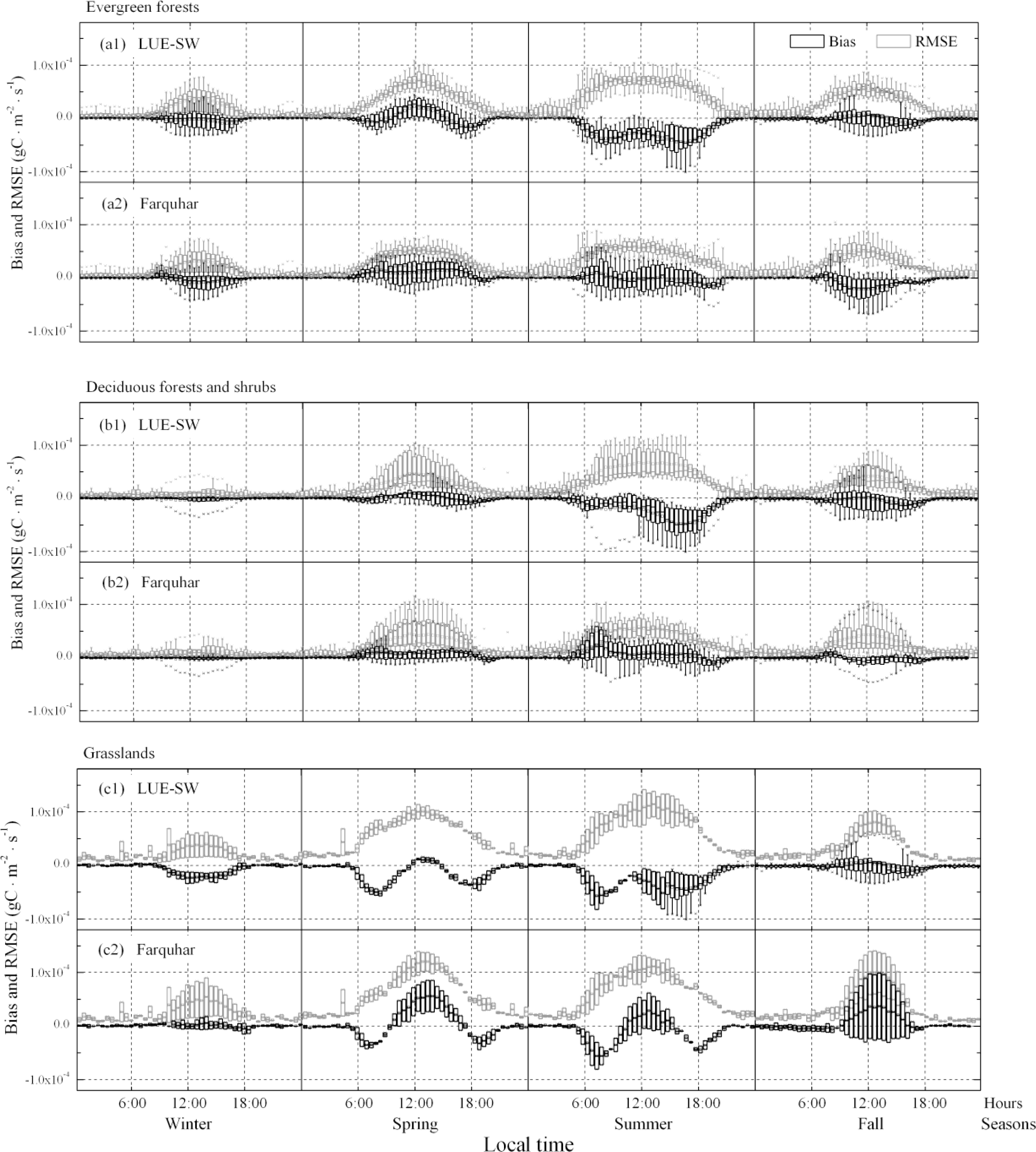
3.2. Model–Data Agreement on Half-Hourly and Daily Time Scales

Two methods of parameter adjustment, optimizing the key parameter ɛ_max and adding the soil water factor, had the same effects on performances of the MODIS GPP algorithm. Examples are presented for one representative year of each site (Table 1) because the behavior is comparable from year to year in each simulation. On half-hourly time scale, σ_norm values tended to increase linearly from 0.77 to 0.97 for LUE and from 0.80 to 0.97 for LUE-SW, in R of 0.74–0.92 and 0.78–0.92, respectively (Figure 1a), indicating that adding the soil water factor to the algorithm could only improve GPP simulation slightly. The two-leaf simulation could well quantify canopy carbon assimilation, in which the average R and σ_norm were 0.882(±0.042) and 1.007(±0.118), respectively, on a half-hourly time scale. LUE and LUE-SW still had same performances after accumulating half-hourly GPP into 8-daily average values (Figure 1b). Note that although the key parameters had been optimized for all three models at each site, the standard deviations of estimates by two one-leaf models were lower than those of observation systematically. The average σ_norm values in LUE-SW decreased by 0.102 and 0.162 on half-hourly and 8-day average time scales, respectively, compared with the two-leaf model. These analyses suggest that parameter optimization is available for compensating the error caused by ignoring soil moisture, but is not for the model structural errors caused by the canopy upscaling strategy.

Moreover, we quantified differences among MOD17A2, LUE_def and three parameter-adjusted simulations (Figure 1b). Site-specific parameters made the simulations more robust than when default values for light use efficiency models were used overall. For most sites we selected, σ_norm, which were ranged from 0.55 to 1.12, increased with R in MOD17A2. The excluded sites are the CA-NS1 (site number 10), FR-Pue (site number 12), IT-Cpz (site number 13), DK-Sor (site number 17), CA-Mer (site number 18), and CA-NS6 (site numbers 19), most of which are deciduous ecosystems. There was no consistency in sites with large or small σ_norm between LUE_def and MOD17A2. For instance, in the CA-NS1 site, σ_norm increased by 0.45 from LUE (0.76) to LUE_def (1.21), and then by 0.70 from LUE_def to MOD17A2 (1.91), which were similar for FR-Pue and CA-NS6. In the ES-ES1 site (site number 5), the value increased by 0.40 from LUE (1.19) to LUE_def (1.59), but decreased by 0.25 from LUE to MOD17A2 (0.94). These results implied that poor parameterization is one reason for errors in MOD17A2, but not for all sites. Errors introduced by parameters could be compensated or intensified by uncertainty in meteorological and vegetation data.

We further compared the daily simulations with the EC observations using the linear regression analyses for each PFT, as shown in Figure 2, whereas the daily observations were averaged into 8-day values to compare with MOD17A2. The slopes of the MODIS product varied largely from 0.49 to 1.50, and the R² ranged from 0.46 to 0.89. Adopting site-specific parameters and input data effectively improved the accuracy of simulations. Further improvements in both correlation and variability were achieved by using the two-leaf strategy. The biases of GPP simulated by the two-leaf Farquhar model were relatively small for nine PFTs, with the slopes of 0.81–1.07 and R² of 0.67–0.92. Overall, model–data agreement across the selected 21 sites was better for the two-leaf model than for the one-leaf model. Systematic underestimation existed in the one-leaf models for all PFTs, and could not be compensated by adjusting key parameters.

3.3. Model–Data Agreement on Monthly and Seasonal Time Scales

We compared monthly and seasonal GPP variation among the simulations to explore the model’s responses to varying weather conditions during different seasons.

Table 3. Bias and root-mean-square error (RMSE) of daily GPP (in gC·m⁻²·day⁻¹) with respect to individual months and seasons.

Months/Seasons	MOD17A2		LUE		LUE-SW		Farquhar
	Bias	RMSE	Bias	RMSE	Bias	RMSE	Bias	RMSE
Jan.	−0.28(±0.43) a	0.42(±0.39)	−0.36(±0.56)	0.49(±0.54)	−0.31(±0.46)	0.43(±0.47)	−0.26(±0.45)	0.43(±0.44)
Feb.	−0.18(±0.48)	0.42(±0.43)	−0.18(±0.65)	0.56(±0.54)	−0.15(±0.54)	0.47(±0.49)	−0.12(±0.59)	0.49(±0.47)
Mar.	−0.28(±0.98)	0.81(±0.78)	−0.11(±0.91)	0.81(±0.61)	−0.09(±0.57)	0.57(±0.42)	0.15(±0.95)	0.80(±0.74)
Apr.	−0.15(±1.91)	1.53(±1.31)	0.31(±1.28)	1.22(±0.77)	0.37(±0.98)	1.01(±0.62)	0.76(±1.19)	1.30(±0.87)
May	−0.39(±2.66)	2.36(±1.69)	−0.62(±1.30)	1.59(±0.96)	−0.42(±1.35)	1.58(±0.95)	0.68(±1.35)	1.48(±0.95)
Jun.	−0.49(±3.08)	2.68(±2.00)	−1.52(±1.33)	2.06(±1.10)	−1.45(±1.21)	1.80(±1.09)	0.19(±1.30)	1.45(±1.02)
Jul.	−0.33(±3.06)	2.70(±1.76)	−1.71(±1.38)	2.02(±1.17)	−1.69(±1.30)	1.92(±1.06)	−0.36(±1.21)	1.42(±0.62)
Aug.	0.08(±2.44)	2.16(±1.48)	−1.18(±1.29)	1.62(±0.97)	−1.03(±1.14)	1.53(±0.85)	−0.54(±0.92)	1.23(±0.54)
Sep.	−0.04(±1.75)	1.61(±1.07)	−0.71(±0.85)	1.19(±0.54)	−0.82(±0.95)	1.30(±0.62)	−0.38(±1.10)	1.16(±0.72)
Oct.	−0.28(±1.03)	0.93(±0.65)	−0.45(±0.88)	0.87(±0.60)	−0.43(±0.90)	0.88(±0.61)	−0.11(±1.21)	0.96(±0.83)
Nov.	−0.22(±0.52)	0.51(±0.38)	−0.19(±0.66)	0.63(±0.45)	−0.15(±0.65)	0.61(±0.46)	0.00(±0.71)	0.60(±0.52)
Dec.	−0.08(±0.58)	0.39(±0.47)	−0.08(±0.46)	0.38(±0.37)	−0.06(±0.51)	0.38(±0.43)	0.03(±0.55)	0.39(±0.45)
Winter b	−0.18(±0.44)	0.43(±0.40)	−0.20(±0.42)	0.52(±0.44)	−0.17(±0.35)	0.77(±0.38)	−0.12(±0.34)	0.47(±0.42)
Spring	−0.21(±0.98)	1.02(±0.81)	−0.02(±0.78)	0.95(±0.51)	0.01(±0.47)	2.05(±0.98)	0.22(±0.69)	0.96(±0.58)
Summer	−0.40(±2.71)	2.66(±1.70)	−1.28(±1.00)	1.96(±0.96)	−1.21(±0.88)	1.57(±0.70)	0.17(±0.90)	1.54(±0.69)
Fall	−0.06(±1.59)	1.81(±0.95)	−0.81(±0.66)	1.36(±0.60)	−1.08(±0.68)	0.47(±0.42)	−0.36(±0.80)	1.21(±0.54)
All year	−0.22(±1.25)	1.78(±0.96)	−0.59(±0.37)	1.38(±0.51)	−0.66(±0.38)	0.43(±0.47)	−0.01(±0.47)	1.18(±0.44)

Note:

^aValues in parentheses are standard deviations.

^bWinter is composed of December, January and February with one year divided into four seasons.

shows that uncertainties of four estimates were large in the warm season. Although the MODIS product had relatively small biases from April to September compared with the other simulations, its standard deviation was 18.6(±15.9) times greater than the value of bias on average, and the RMSE ranged from 1.53 to 2.70 gC·m⁻²·day⁻¹. Thus the low bias of MOD17A2 was caused by terms with opposite signs cancelling anthers. The standard deviations of the biases and the RMSE were relatively small in the other three simulations during the warm season, indicating that the biases could be considered as a measure of modeling uncertainties. LUE underestimated GPP for all seasons, especially in summer, when the bias was −1.28(±1.00) gC·m⁻²·day⁻¹. The negative bias in summer was also apparent for LUE-SW, but it was slightly better. The bias in summer was canceled using the two-leaf Farquhar model with reduced RMSE. However, there were both overestimation in spring and underestimation in autumn for the Farquhar model overall, even though the leaf maximum carboxylation rate has been optimized for each site.

Photosynthesis in winter accounts for ∼7% of yearly carbon assimilation in the selected 11 evergreen forests, and the contribution is as high as 16.6% at the ES-ES1 site. Thus, we further compared the seasonal GPP simulations of this biome type in Figure 3a. Ignoring the MODIS product, the site-level model–data agreement exhibited a low degree of variability from spring to fall, but the Taylor skill ranged from zero to unity in winter, indicating that photosynthesis dynamic could not be captured well during the cold season. The MODIS product for the evergreen forests had a relatively large Taylor skill, but agreed well with observations decreased for the deciduous forests and shrubs (Figure 3b) and the grasslands (Figure 3c) in all four seasons, especially summer, which contributed to the large RMSE indicated in Table 3.

We compared the biases and RMSE of seasonally composite diurnal variations estimated by the LUE-SW and the Farquhar model to find further discrepancies between the simulations (Figure 4). Overall with site-specific parameters (Table 2), both models had similar half-hourly biases and RMSE in all four seasons, excluding obvious underestimations by LUE-SW during the morning and afternoon of summer. The negative biases were improved using the two-leaf Farquhar model with reduced RMSE, especially in the deciduous forests and shrubs. The average biases increased from −35.2(±24.0) to −0.8(±21.5) μgC·m⁻²·s⁻¹ and RMSE decreased from 43.3(±35.8) to 39.0(±32.4) μgC·m⁻²·s⁻¹ during daytime (6:00–18:00) for forests and shrubs in summer (Figure 4a,b). However, a significant improvement by the two-leaf model did not perform in the grasslands (Figure 4c). Note that the estimates by both models had great RMSE during the midday of spring and fall for all biome types, and during the midday of winter for evergreen forests. These results suggest that, whether model structures are complex or simple, the photosynthetic models could not well capture change of GPP consistently in spring and fall for forests and shrubs, and seasonal change for grasslands.

4. Discussion

4.1. Uncertainties in Input Data and Parameters in MOD17A2

Many studies have demonstrated that the MODIS product normally underestimates GPP compared with the EC observations, including savanna and grassland in Africa [14], and forest, grassland and cropland in east Asia [12,13,27,87] and in North America [22,24,88]. However, yearly overestimations were also found at some forest sites [8,13,89,90]. In this study, overestimated and underestimated GPP were both observed at the selected sites (Figure 2), especially in the deciduous forests and shrubs (Figure 3b). It raises doubts as to the accuracy of the simulated temporal and spatial distributions of the MODIS GPP product at regional or global scale because of errors introduced by the reanalysis of meteorological data [65], the fraction of photosynthetically active radiation (fPAR in Equation (1)) [8,14,71], the land cover data [14,91] and the model structure [24,71].

Replacing the reanalysis meteorological and MODIS vegetation data [5,65] with the tower data (LUE_def) did not obviously improve GPP simulations (Figure 1b). Large and small σ_norm were both observed in LUE_def, and the sites with large errors were not consistent with those in MOD17A2 (Figure 1b). For some sites, such as ES-ES1, CA-Oas, CA-Mer, AT-Neu and IE-Dri, the performances were even worse in LUE_def than in MOD17A2. Combining the tower observations with the default parameters in BPLUT [20] could compensate errors introduced by the biome-dependent parameters for some sites, such as ES-ES1, but would increase errors for others, as CA-NS1, FR-Pue and CA-NS6 (Figure 1b). Adjusting parameters using tower data could effectively improve GPP estimate by the MODIS algorithm, but systematic underestimations were observed (Figure 2), thereby indicating model structural errors.

4.2. Uncertainties in Parameter Sets in the MODIS GPP Algorithm

We adjusted the key parameter ɛ_max in the models that based on the MODIS GPP algorithm (LUE and LUE-SW) at site level. The values in LUE-SW were greater than those in LUE on average, but both were not significantly different from the default values except for CA-Oas, DK-Sor, CA-Mer and AT-Neu, for which the value of ɛ_max was greater than 1.3 gC·MJ⁻¹ (Table 2). These sites include the biome types of shrub, grassland and deciduous forest. Overall, the optimized ɛ_max values in both models were in the range of 0.55–2.8 gC·MJ⁻¹, as reported by Garbulsky et al. [92], who calculated the global gross radiation use efficiency from the data provided by 35 EC flux sites and the MODIS fPAR data. Many studies have optimized ɛ_max in the MODIS GPP algorithm based on site data [14,27]. Those results have also demonstrated that the values for shrub and grassland were larger than those in the look-up table, and ɛ_max reached ∼1.56 gC·MJ⁻¹ for deciduous forests [93].

Our values of ɛ_max are acceptable, but an overestimated ɛ_max could be induced by an underestimated fPAR value [14]. In this study, fPAR was calculated based on a function of LAI and k (Equation (2)). Although we corrected the input LAI based on the site-measured LAI_max (Table 1), uncertainties in the change of LAI with phenology still existed at the site level because the monthly data were extracted from a global LAI map [4]. In Equation (2), we simplified the k as 0.5 across a range of biome types. However, this value is dependent on the leaf distribution [94] and the zenith angle, which ranged between 0.3 and 0.6 [95]. The best estimates of k would be derived from stands with minimal clumping for each site [94,95].

4.3. Link between Parameter Sets and Model Structures

A revision of parameters in GPP simulation could cancel errors caused by model structure, including coupled stomatal conductance and carbon assimilation scheme [7], two-stream radiative transfer, and leaf photosynthesis [2]. We evaluated the application of parameter adjustment in the MODIS land algorithm. The results demonstrated that the performances of parameter-optimized LUE and LUE-SW were identical in terms of GPP estimation (Figure 1), but the optimized ɛ_max in the latter model had lower standard deviation than the former for sites within the same PFT (Table 2), even though the parameters categorized according to PFTs are not the best option. After optimizing parameters in simple photosynthesis and transpiration models using measurements from 101 EC flux towers, Groenendijk et al. [81] pointed out that a simple PFT classification could induce the uncertainties in the photosynthesis and water vapor flux estimates, and site-year parameters gave the best predictions. However, this parameter uncertainty could be reduced by adding control factors, such as considering the scale of soil moisture in the one-leaf model (Table 2). Furthermore, we quantified the relationships between annual average soil water factors with optimized ɛ_max in LUE and in LUE-SW, excluding four sites for which ɛ_max was greater than 1.3 gC·MJ⁻¹ (Figure 5). The regression analysis shows that the ɛ_max in LUE decreased linearly with the soil water factor. The reduction was as much as a half in LUE-SW, as evidenced by the slopes reducing from 0.77 to 0.38 and by the constants increasing from 0.32 to 0.73, especially for sites with low annual average soil water factors and large soil water changes. It should be noted that the annual rainfall values of our selected sites were all greater than 200 mm·yr⁻¹ (Table 1). More validations were needed in those water-limited regions with annual precipitation less than 100 mm·yr⁻¹[8,96].

Moreover, parameter adjustment could not compensate all structural errors, such as the error caused by the canopy upscaling strategy. Although we optimized the parameters using data assimilation, GPP estimated by both LUE and LUE-SW still had large negative biases in summer (Table 3). The biases were reduced by 81.9% using the two-leaf Farquhar model. Schaefer et al. [36] compared 26 models with standard parameters at 39 EC flux tower sites across North America and found that the average GPP bias was −0.87 gC·m⁻²·day⁻¹ in summer (Figure 2a), which is between the biases of LUE-SW (−1.21 gC·m⁻²·day⁻¹) and the Farquhar model (0.17 gC·m⁻²·day⁻¹) in the same season that we estimated (Table 3). In their study, more than half of the models adopted the one-leaf upscaling strategy. An underestimation in the MODIS GPP product during summer was also reported by Zhang et al. [24], who evaluated different regions across the conterminous U.S. The reason for underestimation is that the one-leaf strategy ignores a large contribution of diffuse PAR to the shaded leaves, and the contribution is more efficiently absorbed by the canopy for photosynthesis than direct PAR. In the strategy of separating the canopy into two parts, the sunlit leaves achieve a high rate of light-saturated photosynthesis and have a low light use efficiency, whereas shaded leaves are only limited by the electron transport related to direct and diffused radiation, which lead to a high light use efficiency [25,73,97,98]. Many efforts have been made to improve the structure of the MODIS land algorithm by considering photosynthesis rate saturation or light saturation. Propastin et al. [71] adopted a saturating function for light use efficiency adjustment that allowed for saturation of gross photosynthesis at a high irradiance. This modification improved the performance of the MODIS GPP algorithm for a tropical forest. Separating the canopy into sunlit and shaded leaves, He et al. [13,15] developed a two-leaf light use efficiency model based on the MODIS algorithm, and the model properly described differences in the light use efficiencies of sunlit and shaded leaves.

Further improvement should focus on the photosynthesis models’ capacities in capturing seasonal change. In this study, all models exhibited large uncertainties in winter and spring, even if the key parameters in the two-leaf Farquhar model have been well optimized (Table 3, Figures 3 and 4). This result is the same as the simulations from 26 models at 39 EC sites [36]. Fortunately, many approaches could be referred to quantify seasonal variation of key variables in GPP estimates. A comparison between using the dynamic maximum velocity of carboxylation (Vc_max in Equation (A3)) and the constant Vc_max in the Farquhar models by Muraoka et al. [99] indicated that Vc_max variation had remarkable effects on GPP, and an overestimate of 15% was caused by assuming Vc_max to be constant in a cool-temperate deciduous broadleaf forest. Groenendijk et al. [100] upscaled the ecosystem parameters Vc_max with LAI for 81 EC sites, but the seasonal variation of Vc_max could not be sufficiently explained at the ecosystem scale. By seasonally changing the photosynthetic parameters in a Farquhar-type biochemical model, Zhu et al. [101] successfully reproduced the observed response in net assimilation rates at leaf scale. According to satellite data and the Biome-BGC terrestrial ecosystem model, Ichii et al. [102] suggested that proper setting of the root depths was important to simulate GPP seasonality in tropical forests. On the basis of these studies, a widely accepted concept is needed to improve seasonal change in GPP estimate.

5. Conclusions

By comparing GPP estimates with parameter adjustment in the MODIS algorithm across nine PFTs at half-hourly, daily, monthly and seasonal scales, our multisite study illustrates as follows:

(1)

Large bias was observed in the MODIS GPP product, especially in deciduous forests and shrubs and grasslands. Its uncertainties were affected by both input data and the look-up table values of ɛ_max for individual PFTs. It is necessary to optimize the parameters in the look-up table used by the MODIS algorithm, but the optimized parameters should correspond to specific input data for applications, i.e., the optimized parameters cannot be applied to a simulation with changed driver data because errors from parameters and input data can accumulate.

(2)

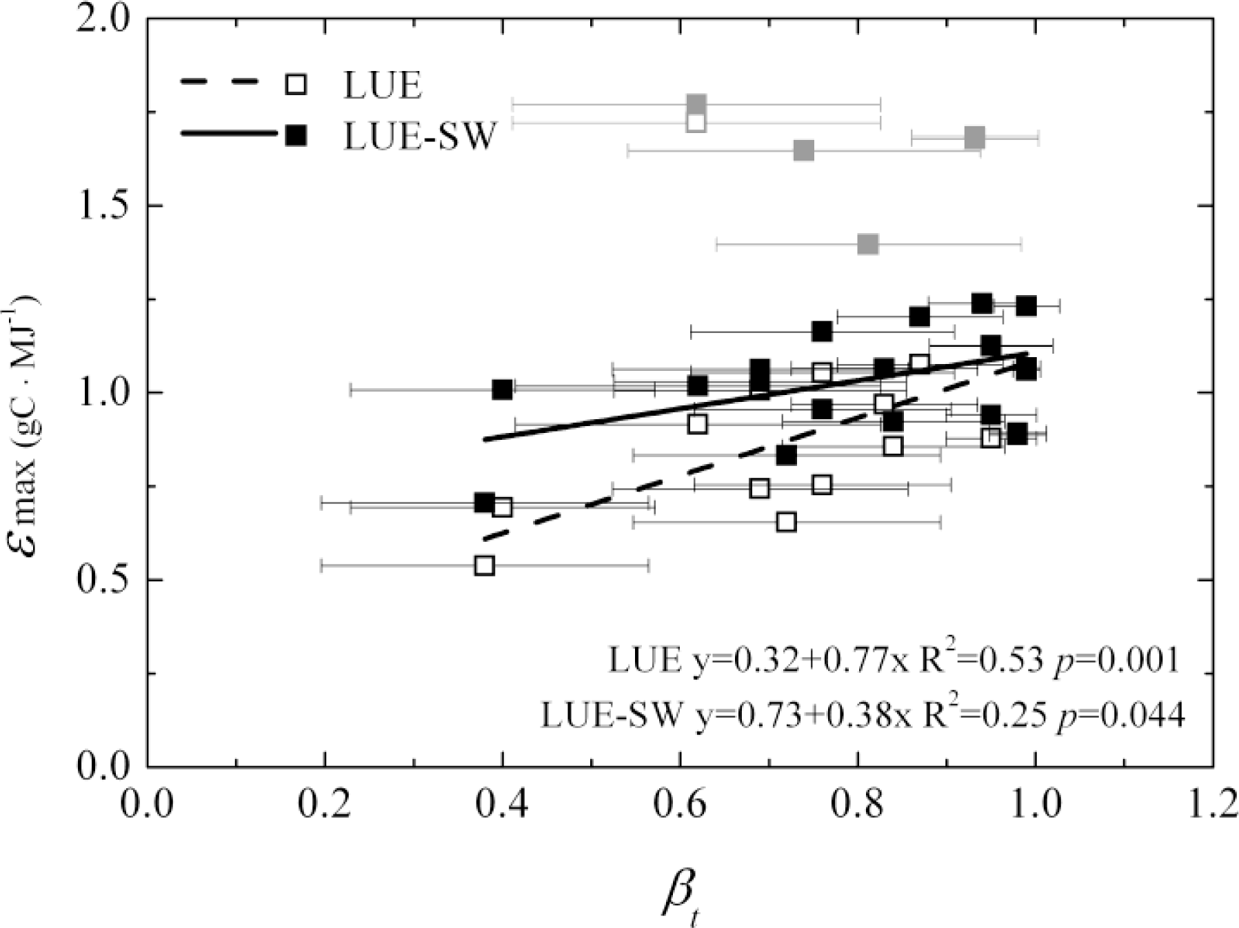
Optimizing the key parameter ɛ_max in the MODIS GPP algorithm can compensate the errors caused by ignoring soil water factor at the site level, but the ɛ_max values would have large uncertainties among sites within the same PFT and among the PFTs, especially for sites with low yearly average soil water factors. This result casts doubt on the accuracy of simulated spatial distribution of GPP yielded by the MODIS algorithm. Moreover, GPP was underestimated by the one-leaf models in summer, regardless of whether the soil water factor was considered, but could be improved by separating the canopy structure into sunlit and shaded parts. This result indicates that improving model structure is a better choice than only adjusting parameters. Photosynthetic dynamics in spring and fall for forests and shrubs and seasonal GPP change for grasslands could not be captured by both one-leaf and two-leaf models. Therefore, there is a need to improve seasonal and phenology variations of key parameters and variables in carbon assimilation calculation to reduce uncertainties in GPP simulation.

References

1. Beer, C.; Reichstein, M.; Tomelleri, E.; Ciais, P.; Jung, M.; Carvalhais, N.; Rodenbeck, C.; Arain, M.A.; Baldocchi, D.; Bonan, G.B.; et al. Terrestrial gross carbon dioxide uptake: Global distribution and covariation with climate. Science 2010, 329, 834–838. [Google Scholar]
2. Bonan, G.B.; Lawrence, P.J.; Oleson, K.W.; Levis, S.; Jung, M.; Reichstein, M.; Lawrence, D.M.; Swenson, S.C. Improving canopy processes in the Community Land Model version 4 (CLM4) using global flux fields empirically inferred from fluxnet data. J. Geophys. Res 2011. [Google Scholar] [CrossRef]
3. Jung, M.; Reichstein, M.; Margolis, H.A.; Cescatti, A.; Richardson, A.D.; Arain, M.A.; Arneth, A.; Bernhofer, C.; Bonal, D.; Chen, J.; et al. Global patterns of land-atmosphere fluxes of carbon dioxide, latent heat, and sensible heat derived from eddy covariance, satellite, and meteorological observations. J. Geophys. Res 2011. [Google Scholar] [CrossRef]
4. Chen, J.M.; Mo, G.; Pisek, J.; Liu, J.; Deng, F.; Ishizawa, M.; Chan, D. Effects of foliage clumping on the estimation of global terrestrial gross primary productivity. Glob. Biogeochem. Cy 2012. [Google Scholar] [CrossRef]
5. Zhao, M.; Heinsch, F.A.; Nemani, R.R.; Running, S.W. Improvements of the MODIS terrestrial gross and net primary production global data set. Remote Sens. Environ 2005, 95, 164–176. [Google Scholar]
6. Piao, S.; Sitch, S.; Ciais, P.; Friedlingstein, P.; Peylin, P.; Wang, X.; Ahlstrom, A.; Anav, A.; Canadell, J.G.; Cong, N.; et al. Evaluation of terrestrial carbon cycle models for their response to climate variability and to CO2 trends. Glob. Change Biol 2013, 19, 2117–2132. [Google Scholar]
7. Chen, H.; Dickinson, R.E.; Dai, Y.; Zhou, L. Sensitivity of simulated terrestrial carbon assimilation and canopy transpiration to different stomatal conductance and carbon assimilation schemes. Clim. Dynam 2010, 36, 1037–1054. [Google Scholar]
8. Kanniah, K.D.; Beringer, J.; Hutley, L.B.; Tapper, N.J.; Zhu, X. Evaluation of collections 4 and 5 of the MODIS gross primary productivity product and algorithm improvement at a tropical savanna site in northern Australia. Remote Sens. Environ 2009, 113, 1808–1822. [Google Scholar]
9. Monteith, J.L. Solar radiation and productivity in tropical ecosystems. J. Appl. Ecol 1972, 9, 747–766. [Google Scholar]
10. Farquhar, G.D.; Caemmerer, S.V.; Berry, J.A. A biochemical model of photosynthetic CO2 assimilation in leaves of C3 species. Planta 1980, 149, 78–90. [Google Scholar]
11. Beer, C.; Reichstein, M.; Ciais, P.; Farquhar, G.D.; Papale, D. Mean annual GPP of Europe derived from its water balance. Geophys. Res. Lett 2007. [Google Scholar] [CrossRef]
12. Thurner, M.; Beer, C.; Santoro, M.; Carvalhais, N.; Wutzler, T.; Schepaschenko, D.; Shvidenko, A.; Kompter, E.; Ahrens, B.; Levick, S.R.; et al. Carbon stock and density of northern boreal and temperate forests. Glob. Ecol. Biogeogr 2013. [Google Scholar] [CrossRef]
13. He, M.; Zhou, Y.; Ju, W.; Chen, J.; Zhang, L.; Wang, S.; Saigusa, N.; Hirata, R.; Murayama, S.; Liu, Y. Evaluation and improvement of MODIS gross primary productivity in typical forest ecosystems of east Asia based on eddy covariance measurements. J. Forest Res 2013, 18, 31–40. [Google Scholar]
14. Sjöström, M.; Zhao, M.; Archibald, S.; Arneth, A.; Cappelaere, B.; Falk, U.; de Grandcourt, A.; Hanan, N.; Kergoat, L.; Kutsch, W.; et al. Evaluation of MODIS gross primary productivity for Africa using eddy covariance data. Remote Sens. Environ 2013, 131, 275–286. [Google Scholar]
15. He, M.; Ju, W.; Zhou, Y.; Chen, J.; He, H.; Wang, S.; Wang, H.; Guan, D.; Yan, J.; Li, Y.; et al. Development of a two-leaf light use efficiency model for improving the calculation of terrestrial gross primary productivity. Agric. Forest Meteorol 2013, 173, 28–39. [Google Scholar]
16. Yuan, W.; Liu, S.; Zhou, G.; Zhou, G.; Tieszen, L.L.; Baldocchi, D.; Bernhofer, C.; Gholz, H.; Goldstein, A.H.; Goulden, M.L.; et al. Deriving a light use efficiency model from eddy covariance flux data for predicting daily gross primary production across biomes. Agric. Forest Meteorol 2007, 143, 189–207. [Google Scholar]
17. Xiao, X.; Zhang, Q.; Hollinger, D.; Aber, J.; Moore, B. Modeling gross primary production of an evergreen needleleaf forest using MODIS and climate data. Ecol. Appl 2005, 15, 954–969. [Google Scholar]
18. Wu, C.; Munger, J.W.; Niu, Z.; Kuang, D. Comparison of multiple models for estimating gross primary production using MODIS and eddy covariance data in harvard forest. Remote Sens. Environ 2010, 114, 2925–2939. [Google Scholar]
19. Heinsch, F.A.; Reeves, M.; Votava, P.; Kang, S.; Milesi, C.; Zhao, M.; Glassy, J.; Jolly, W.M.; Loehman, R.; Bowker, C.F.; et al. User’s Guide GPP and NPP (MOD17A2/A3) Products NASA MODIS Land Algorithm; Version 2.0; MODIS Land Team: Washington, DC, USA, 2003; p. 17. [Google Scholar]
20. Zhao, M.; Running, S.W. Drought-induced reduction in global terrestrial net primary production from 2000 through 2009. Science 2010, 329, 940–943. [Google Scholar]
21. Turner, D.P.; Ritts, W.D.; Cohen, W.B.; Gower, S.T.; Zhao, M.; Running, S.W.; Wofsy, S.C.; Urbanski, S.; Dunn, A.L.; Munger, J.W. Scaling gross primary production (GPP) over boreal and deciduous forest landscapes in support of MODIS GPP product validation. Remote Sens. Environ 2003, 88, 256–270. [Google Scholar]
22. Sims, D.; Rahman, A.; Cordova, V.; Elmasri, B.; Baldocchi, D.; Bolstad, P.; Flanagan, L.; Goldstein, A.; Hollinger, D.; Misson, L. A new model of gross primary productivity for north American ecosystems based solely on the enhanced vegetation index and land surface temperature from MODIS. Remote Sens. Environ 2008, 112, 1633–1646. [Google Scholar]
23. Wu, C.; Niu, Z.; Gao, S. Gross primary production estimation from MODIS data with vegetation index and photosynthetically active radiation in maize. J. Geophys. Res 2010. doi: 12110.11029/12009JD013023. [Google Scholar]
24. Zhang, F.; Chen, J.M.; Chen, J.; Gough, C.M.; Martin, T.A.; Dragoni, D. Evaluating spatial and temporal patterns of MODIS GPP over the conterminous U.S. Against flux measurements and a process model. Remote Sens. Environ 2012, 124, 717–729. [Google Scholar]
25. Dai, Y.; Dickinson, R.E.; Wang, Y.P. A two-big-leaf model for canopy temperature, photosynthesis and stomatal conductance. J. Clim 2004, 17, 2281–2299. [Google Scholar]
26. Sprintsin, M.; Chen, J.M.; Desai, A.; Gough, C.M. Evaluation of leaf-to-canopy upscaling methodologies against carbon flux data in north america. J. Geophys. Res 2012. [Google Scholar] [CrossRef]
27. Wang, X.; Ma, M.; Li, X.; Song, Y.; Tan, J.; Huang, G.; Zhang, Z.; Zhao, T.; Feng, J.; Ma, Z.; et al. Validation of MODIS-GPP product at 10 flux sites in northern China. Int. J. Remote Sens 2013, 34, 587–599. [Google Scholar]
28. Hashimoto, H.; Wang, W.; Milesi, C.; Xiong, J.; Ganguly, S.; Zhu, Z.; Nemani, R. Structural uncertainty in model-simulated trends of global gross primary production. Remote Sens 2013, 5, 1258–1273. [Google Scholar]
29. Mäkelä, A.; Pulkkinen, M.; Kolari, P.; Lagergren, F.; Berbigier, P.; Lindroth, A.; Loustau, D.; Nikinmaa, E.; Vesala, T.; Hari, P. Developing an empirical model of stand GPP with the LUE approach: Analysis of eddy covariance data at five contrasting conifer sites in Europe. Glob. Chang. Biol 2008, 14, 92–108. [Google Scholar]
30. Mu, Q.; Zhao, M.; Heinsch, F.A.; Liu, M.; Tian, H.; Running, S.W. Evaluating water stress controls on primary production in biogeochemical and remote sensing based models. J. Geophys. Res 2007. [Google Scholar] [CrossRef]
31. Keenan, T.F.; Davidson, E.; Moffat, A.M.; Munger, W.; Richardson, A.D. Using model-data fusion to interpret past trends, and quantify uncertainties in future projections, of terrestrial ecosystem carbon cycling. Glob. Chang. Biol 2012, 18, 2555–2569. [Google Scholar]
32. Chen, B.; Chen, J.M.; Ju, W. Remote sensing-based ecosystem–atmosphere simulation scheme (EASS)—Model formulation and test with multiple-year data. Ecol. Model 2007, 209, 277–300. [Google Scholar]
33. Chen, J.; Chen, B.; Black, T.A.; Innes, J.L.; Wang, G.; Kiely, G.; Hirano, T.; Wohlfahrt, G. Comparison of terrestrial evapotranspiration estimates using the mass-transfer and Penman-Monteith equations in land-surface models. J. Geophys. Res 2013. [Google Scholar] [CrossRef]
34. Wilson, K.B.; Goldstein, A.; Falge, E.; Aubinet, M.; Baldocchi, D.; Berbigier, P.; Bernhofer, C.; Ceulemans, R.; Dolman, H.; Field, C.; et al. Energy balance closure at fluxnet sites. Agric. Forest Meteorol 2002, 113, 223–243. [Google Scholar]
35. Stoy, P.C.; Mauder, M.; Foken, T.; Marcolla, B.; Boegh, E.; Ibrom, A.; Arain, M.A.; Arneth, A.; Aurela, M.; Bernhofer, C.; et al. A data-driven analysis of energy balance closure across fluxnet research sites: The role of landscape scale heterogeneity. Agric. Forest Meteorol 2013, (171–172), 137–152. [Google Scholar]
36. Schaefer, K.; Schwalm, C.R.; Williams, C.; Arain, M.A.; Barr, A.; Chen, J.M.; Davis, K.J.; Dimitrov, D.; Hilton, T.W.; Hollinger, D.Y.; et al. A model-data comparison of gross primary productivity: Results from the north American carbon program site synthesis. J. Geophys. Res 2012. [Google Scholar] [CrossRef]
37. Oleson, K.W.; Lawrence, D.M.; Bonan, G.B.; Flanner, M.G.; Kluzek, E.; Lawrence, P.J.; Levis, S.; Swenson, S.C.; Thornton, P.E.; Dai, A.; et al. Technical Description of Version 4.0 of the Community Land Model (CLM); National Center for Atmospheric Research: Boulder, CO, USA, 2010. [Google Scholar]
38. Chen, B.; Coops, N.C.; Andy Black, T.; Jassal, R.S.; Chen, J.M.; Johnson, M. Modeling to discern nitrogen fertilization impacts on carbon sequestration in a pacific northwest douglas-fir forest in the first-postfertilization year. Glob. Chang. Biol 2011, 17, 1442–1460. [Google Scholar]
39. Krishnan, P.; Black, T.A.; Jassal, R.S.; Chen, B.; Nesic, Z. Interannual variability of the carbon balance of three different-aged douglas-fir stands in the pacific northwest. J. Geophys. Res 2009. [Google Scholar] [CrossRef]
40. Grant, R.F.; Barr, A.G.; Black, T.A.; Margolis, H.A.; McCaughey, J.H.; Trofymow, J.A. Net ecosystem productivity of temperate and boreal forests after clearcutting a fluxnet-Canada measurement and modelling synthesis. Tellus B 2010, 62, 475–496. [Google Scholar]
41. Grünwald, T.; Bernhofer, C. A decade of carbon, water and energy flux measurements of an old spruce forest at the Anchor Station Tharandt. Tellus B 2007, 59, 387–396. [Google Scholar]
42. Blyth, E.; Gash, J.; Lloyd, A.; Pryor, M.; Weedon, G.P.; Shuttleworth, J. Evaluating the JULES land surface model energy fluxes using fluxnet data. J. Hydrometeorol 2010, 11, 509–519. [Google Scholar]
43. Hollinger, D.Y.; Aber, J.; Dail, B.; Davidson, E.A.; Goltz, S.M.; Hughes, H.; Leclerc, M.Y.; Lee, J.T.; Richardson, A.D.; Rodrigues, C.; et al. Spatial and temporal variability in forest-atmosphere CO2 exchange. Glob. Chang. Biol 2004, 10, 1689–1706. [Google Scholar]
44. Li, X.; Liu, Q.; Cai, Z.; Ma, Z. Specificleaf area and leaf area index of conifer plantations in Qianyanzhou station of subtropical China. J. Plant Ecol 2007, 31, 93–101. (In Chinese) [Google Scholar]
45. Bergeron, O.; Margolis, H.A.; Black, T.A.; Coursolle, C.; Dunn, A.L.; Barr, A.G.; Wofsy, S.C. Comparison of carbon dioxide fluxes over three boreal black spruce forests in Canada. Glob. Chang. Biol 2007, 13, 89–107. [Google Scholar]
46. Kljun, N.; Black, T.A.; Griffis, T.J.; Barr, A.G.; Gaumont-Guay, D.; Morgenstern, K.; McCaughey, J.H.; Nesic, Z. Response of net ecosystem productivity of three boreal forest stands to drought. Ecosystems 2006, 9, 1128–1144. [Google Scholar]
47. Gaumont-Guay, D.; Black, T.A.; Barr, A.G.; Griffis, T.J.; Jassal, R.S.; Krishnan, P.; Grant, N.; Nesic, Z. Eight years of forest-floor CO2 exchange in a boreal black spruce forest: spatial integration and long-term temporal trends. Agric. Forest Meteorol 2014, 184, 25–35. [Google Scholar]
48. Hill, T.C.; Williams, M.; Woodward, F.I.; Moncrieff, J.B. Constraining ecosystem processes from tower fluxes and atmospheric profile. Ecol. Appl 2011, 21, 1474–1489. [Google Scholar]
49. Tanja, S.; Berninger, F.; Sala, T.V.; Markkanen, T.I.; Hari, P.; MaKela, A.; Ilvesniemi, H.; Hanninen, H.; Nikinmaa, E.; Huttula, T.; et al. Air temperature triggers the recovery of evergreen boreal forest photosynthesis in spring. Glob. Chang. Biol 2003, 9, 1410–1426. [Google Scholar]
50. Rambal, S.; Ourcival, J.E.-M.; Joffre, R.; Mouillot, F.L.; Nouvellon, Y.; Reichstein, M.; Rocheteauz, A. Drought controls over conductance and assimilation of a mediterranean evergreen ecosystem: scaling from leaf to canopy. Glob. Chang. Biol 2003, 9, 1813–1824. [Google Scholar]
51. Garbulsky, M.F.; PeÑUelas, J.; Papale, D.; Filella, I. Remote estimation of carbon dioxide uptake by a mediterranean forest. Glob. Chang. Biol 2008, 14, 2860–2867. [Google Scholar]
52. Reichstein, M.; Ciais, P.; Papale, D.; Valentini, R.; Running, S.; Viovy, N.; Cramer, W.; Granier, A.; Ogee, J.; Allard, V.; et al. Reduction of ecosystem productivity and respiration during the european summer 2003 climate anomaly: A joint flux tower, remote sensing and modelling analysis. Glob. Chang. Biol 2007, 13, 634–651. [Google Scholar]
53. Valentini, R.; Angelis, P.D.; Matteuci, G.; Monaco, R.; Dore, S.; Mucnozza, G.E.S. Seasonal net carbon dioxide exchange of a beech forest with the atmosphere. Glob. Chang. Biol 1996, 2, 199–207. [Google Scholar]
54. Gu, L.; Meyers, T.; Pallardy, S.G.; Hanson, P.J.; Yang, B.; Heuer, M.; Hosman, K.P.; Riggs, J.S.; Sluss, D.; Wullschleger, S.D. Direct and indirect effects of atmospheric conditions and soil moisture on surface energy partitioning revealed by a prolonged drought at a temperate forest site. J. Geophys. Res 2006. [Google Scholar] [CrossRef]
55. Barr, A.G.; Black, T.A.; Hogg, E.H.; Griffis, T.J.; Morgenstern, K.; Kljun, N.; Theede, A.; Nesic, Z. Climatic controls on the carbon and water balances of a boreal aspen forest, 1994–2003. Glob. Chang. Biol 2007, 13, 561–576. [Google Scholar]
56. Krishnan, P.; Black, T.A.; Grant, N.J.; Barr, A.G.; Hogg, E.H.; Jassal, R.S.; Morgenstern, K. Impact of changing soil moisture distribution on net ecosystem productivity of a boreal aspen forest during and following drought. Agric. Forest Meteorol 2006, 139, 208–223. [Google Scholar]
57. Pilegaard, K.; Ambus, P.; Mikkelsen, T.N.; Beier, C.; Ro-Poulsen, H. Field measurements of atmosphere-biosphere interactions in a danish beech forest. Boreal Environ. Res 2003, 8, 315–333. [Google Scholar]
58. Lafleur, P.M.; Roulet, N.T.; Bubier, J.L.; Frolking, S.; Moore, T.R. Interannual variability in the peatland-atmosphere carbon dioxide exchange at an ombrotrophic bog. Glob. Biogeochem. Cy 2003. [Google Scholar] [CrossRef]
59. Roulet, N.T.; Lafleur, P.M.; Richard, P.J.H.; Moore, T.R.; Humphreys, E.R.; Bubier, J. Contemporary carbon balance and late holocene carbon accumulation in a northern peatland. Glob. Chang. Biol 2007, 13, 397–411. [Google Scholar]
60. Goulden, M.L.; Winston, G.C.; McMillan, A.M.S.; Litvak, M.E.; Read, E.L.; Rocha, A.V.; Rob Elliot, J. An eddy covariance mesonet to measure the effect of forest age on land-atmosphere exchange. Glob. Chang. Biol 2006, 12, 2146–2162. [Google Scholar]
61. McMillan, A.M.S.; Winston, G.C.; Goulden, M.L. Age-dependent response of boreal forest to temperature and rainfall variability. Glob. Chang. Biol 2008, 14, 1904–1916. [Google Scholar]
62. Wohlfahrt, G.; Hammerle, A.; Haslwanter, A.; Bahn, M.; Tappeiner, U.; Cernusca, A. Seasonal and inter-annual variability of the net ecosystem CO2 exchange of a temperate mountain grassland: Effects of weather and management. J. Geophys. Res 2008. doi: 08110.01029/02007JD009286. [Google Scholar]
63. Montaldo, N.; Albertson, J.D.; Mancini, M. Dynamic calibration with an ensemble Kalman filter based data assimilation approach for root-zone moisture predictions. J. Hydrometeorol 2007, 8, 910–921. [Google Scholar]
64. Peichl, M.; Leahy, P.; Kiely, G. Six-year stable annual uptake of carbon dioxide in intensively managed humid temperate grassland. Ecosystems 2010, 14, 112–126. [Google Scholar]
65. Zhao, M.; Running, S.W.; Nemani, R.R. Sensitivity of moderate resolution imaging spectroradiometer (MODIS) terrestrial primary production to the accuracy of meteorological reanalyses. J. Geophys. Res 2006. doi: 01010.01029/02004JG000004. [Google Scholar]
66. Chen, B.; Coops, N.C.; Fu, D.; Margolis, H.A.; Amiro, B.D.; Barr, A.G.; Black, T.A.; Arain, M.A.; Bourque, C.P.A.; Flanagan, L.B.; et al. Assessing eddy-covariance flux tower location bias across the fluxnet-canada research network based on remote sensing and footprint modelling. Agric. Forest Meteorol 2011, 151, 87–100. [Google Scholar]
67. Chasmer, L.; Barr, A.; Hopkinson, C.; McCaughey, H.; Treitz, P.; Black, A.; Shashkov, A. Scaling and assessment of GPP from MODIS using a combination of airborne lidar and eddy covariance measurements over jack pine forests. Remote Sens. Environ 2009, 113, 82–93. [Google Scholar]
68. Xiao, J.; Zhuang, Q.; Law, B.E.; Chen, J.; Baldocchi, D.D.; Cook, D.R.; Oren, R.; Richardson, A.D.; Wharton, S.; Ma, S. A continuous measure of gross primary production for the conterminous united states derived from MODIS and Ameriflux data. Remote Sens. Environ 2010, 114, 576–591. [Google Scholar]
69. Running, S.W.; Nemani, R.R.; Heinsch, F.A.; Zhao, Maosheng; Reeves, M.; Hashimoto, H. A continuous satellite-derived measure of global terrestrial primary production. BioScience 2004, 54, 547–560. [Google Scholar]
70. Turner, D.P.; Ritts, W.D.; Cohen, W.B.; Gower, S.T.; Running, S.W.; Zhao, M.; Costa, M.H.; Kirschbaum, A.A.; Ham, J.M.; Saleska, S.R.; et al. Evaluation of MODIS NPP and GPP products across multiple biomes. Remote Sens. Environ 2006, 102, 282–292. [Google Scholar]
71. Propastin, P.; Ibrom, A.; Knohl, A.; Erasmi, S. Effects of canopy photosynthesis saturation on the estimation of gross primary productivity from MODIS data in a tropical forest. Remote Sens. Environ 2012, 121, 252–260. [Google Scholar]
72. Hu, Z.; Li, S.; Yu, G.; Sun, X.; Zhang, L.; Han, S.; Li, Y. Modeling evapotranspiration by combing a two-source model, a leaf stomatal model, and a light-use efficiency model. J. Hydrol 2013, 501, 186–192. [Google Scholar]
73. Chen, J.M.; Liu, J.; Cihlar, J.; Goulden, M.L. Daily canopy photosynthesis model through temporal and spatial scaling for remote sensing applications. Ecol. Model 1999, 124, 99–119. [Google Scholar]
74. Falge, E.; Baldocchi, D.; Olson, R.; Anthoni, P.; Aubinet, M.; Bernhofer, C.; Burba, G.; Ceulemans, R.; Clement, R.; Dolman, H.; et al. Gap filling strategies for defensible annual sums of net ecosystem exchange. Agric. Forest Meteorol 2001, 107, 43–69. [Google Scholar]
75. Moffat, A.M.; Papale, D.; Reichstein, M.; Hollinger, D.Y.; Richardson, A.D.; Barr, A.G.; Beckstein, C.; Braswell, B.H.; Churkina, G.; Desai, A.R.; et al. Comprehensive comparison of gap-filling techniques for eddy covariance net carbon fluxes. Agric. Forest Meteorol 2007, 147, 209–232. [Google Scholar]
76. Chen, J.M.; Menges, C.H.; Leblanc, S.G. Global mapping of foliage clumping index using multi-angular satellite data. Remote Sens. Environ 2005, 97, 447–457. [Google Scholar]
77. Deng, F.; Chen, J.M.; Plummer, S.; Mingzhen, C.; Pisek, J. Algorithm for global leaf area index retrieval using satellite imagery. IEEE Tran. Geosci. Remote Sens 2006, 44, 2219–2229. [Google Scholar]
78. Qian, T.; Dai, A.; Trenberth, K.E.; Oleson, K.W. Simulation of global land surface conditions from 1948 to 2004. Part I: Forcing data and evaluations. J. Hydrometeorol 2006, 7, 953–975. [Google Scholar]
79. Lawrence, D.M.; Oleson, K.W.; Flanner, M.G.; Thornton, P.E.; Swenson, S.C.; Lawrence, P.J.; Zeng, X.; Yang, Z.L.; Levis, S.; Sakaguchi, K.; et al. Parameterization improvements and functional and structural advances in version 4 of the community land model. J. Adv. Model. Earth Syst 2011. doi: 03010.01029/02011MS000045. [Google Scholar]
80. Mo, X.; Chen, J.M.; Ju, W.; Black, T.A. Optimization of ecosystem model parameters through assimilating eddy covariance flux data with an ensemble kalman filter. Ecol. Model 2008, 217, 157–173. [Google Scholar]
81. Groenendijk, M.; Dolman, A.J.; van der Molen, M.K.; Leuning, R.; Arneth, A.; Delpierre, N.; Gash, J.H.C.; Lindroth, A.; Richardson, A.D.; Verbeeck, H.; et al. Assessing parameter variability in a photosynthesis model within and between plant functional types using global fluxnet eddy covariance data. Agric. Forest Meteorol 2011, 151, 22–38. [Google Scholar]
82. Willmott, C.J. Some comments on the evaluation of model performance. Bull. Am. Meterol. Soc 1982, 63, 1309–1313. [Google Scholar]
83. Willmott, C.J.; Matsuura, K. Advantages of the mean absolute error (MAE) over the root mean square error (RMSE) in assessing average model performance. Clim. Res 2005, 30, 79–82. [Google Scholar]
84. Willmott, C.J.; Ackleson, S.G.; Davis, R.E.; Feddema, J.J.; Klink, K.M.; Legates, D.R.; O’Donnell, J.; Rowe, C.M. Statistics for the evaluation and comparison of models. J. Geophys. Res 1985, 90, 8995–9005. [Google Scholar]
85. Taylor, K.E. Summarizing multiple aspects of model performance in a single diagram. J. Geophys. Res 2001, 106, 7183–7192. [Google Scholar]
86. Schwalm, C.R.; Williams, C.A.; Schaefer, K.; Anderson, R.; Arain, M.A.; Baker, I.; Barr, A.; Black, T.A.; Chen, G.; Chen, J.M.; et al. A model-data intercomparison of CO2 exchange across north America: Results from the north American carbon program site synthesis. J. Geophys. Res 2010. [Google Scholar] [CrossRef] [Green Version]
87. John, R.; Chen, J.; Noormets, A.; Xiao, X.; Xu, J.; Lu, N.; Chen, S. Modelling gross primary production in semi-arid inner Mongolia using MODIS imagery and eddy covariance data. Int. J. Remote. Sens 2013, 34, 2829–2857. [Google Scholar]
88. Coops, N.; Black, T.; Jassal, R.; Trofymow, J.; Morgenstern, K. Comparison of MODIS, eddy covariance determined and physiologically modelled gross primary production (GPP) in a douglas-fir forest stand. Remote Sens. Environ 2007, 107, 385–401. [Google Scholar]
89. Schubert, P.; Lagergren, F.; Aurela, M.; Christensen, T.; Grelle, A.; Heliasz, M.; Klemedtsson, L.; Lindroth, A.; Pilegaard, K.; Vesala, T.; et al. Modeling GPP in the nordic forest landscape with MODIS time series data—Comparison with the MODIS GPP product. Remote Sens. Environ 2012, 126, 136–147. [Google Scholar]
90. Heinsch, F.A.; Zhao, M.; Running, S.W.; Kimball, J.S.; Nemani, R.R.; Davis, K.J.; Bolstad, P.V.; Cook, B.D.; Desai, A.R.; Ricciuto, D.M.; et al. Evaluation of remote sensing based terrestrial productivity from MODIS using regional tower eddy flux network observations. IEEE Tran. Geosci. Remote Sens 2006, 44, 1908–1923. [Google Scholar]
91. Cracknell, A.P.; Kanniah, K.D.; Tan, K.P.; Wang, L. Evaluation of MODIS gross primary productivity and land cover products for the humid tropics using oil palm trees in Peninsular Malaysia and Google Earth imagery. Int. J. Remote Sens 2013, 34, 7400–7423. [Google Scholar]
92. Garbulsky, M.F.; Peñuelas, J.; Papale, D.; Ardö, J.; Goulden, M.L.; Kiely, G.; Richardson, A.D.; Rotenberg, E.; Veenendaal, E.M.; Filella, I. Patterns and controls of the variability of radiation use efficiency and primary productivity across terrestrial ecosystems. Glob. Ecol. Biogeogr 2010, 19, 253–267. [Google Scholar]
93. Yang, F.; Ichii, K.; White, M.A.; Hashimoto, H.; Michaelis, A.R.; Votava, P.; Zhu, A.X.; Huete, A.; Running, S.W.; Nemani, R.R. Developing a continental-scale measure of gross primary production by combining MODIS and Ameriflux data through support vector machine approach. Remote Sens. Environ 2007, 110, 109–122. [Google Scholar]
94. Chen, J.M.; Black, T.A. Measuring leaf-area index of plant canopies with branch architecture. Agric. Forest Meteorol 1991, 57, 1–12. [Google Scholar]
95. Macfarlane, C.; Hoffman, M.; Eamus, D.; Kerp, N.; Higginson, S.; McMurtrie, R.; Adams, M. Estimation of leaf area index in eucalypt forest using digital photography. Agric. Forest Meteorol 2007, 143, 176–188. [Google Scholar]
96. Nightingale, J.M.; Coops, N.C.; Waring, R.H.; Hargrove, W.W. Comparison of MODIS gross primary production estimates for forests across the U.S.A. With those generated by a simple process model, 3-PGS. Remote Sens. Environ 2007, 109, 500–509. [Google Scholar]
97. Pury, D.G.G.D.; Farquhar, G.D. Simple scaling of photosynthesis from leaves to canopies without the errors of big-leaf model. Plant Cell Environ 1997, 20, 537–557. [Google Scholar]
98. Wang, Y.P.; Leuning, R. A two-leaf model for canopy conductance, photosynthesis and partitioning of available energy I: Model description and comparison with a multi-layered model. Agric. Forest Meteorol 1998, 91, 89–111. [Google Scholar]
99. Muraoka, H.; Saigusa, N.; Nasahara, K.N.; Noda, H.; Yoshino, J.; Saitoh, T.M.; Nagai, S.; Murayama, S.; Koizumi, H. Effects of seasonal and interannual variations in leaf photosynthesis and canopy leaf area index on gross primary production of a cool-temperate deciduous broadleaf forest in Takayama, Japan. J. Plant Res 2010, 123, 563–576. [Google Scholar]
100. Groenendijk, M.; Dolman, A.J.; Ammann, C.; Arneth, A.; Cescatti, A.; Dragoni, D.; Gash, J.H.C.; Gianelle, D.; Gioli, B.; Kiely, G.; et al. Seasonal variation of photosynthetic model parameters and leaf area index from global fluxnet eddy covariance data. J. Geophys. Res 2011. [Google Scholar] [CrossRef]
101. Zhu, G.F.; Li, X.; Su, Y.H.; Lu, L.; Huang, C.L. Seasonal fluctuations and temperature dependence in photosynthetic parameters and stomatal conductance at the leaf scale of populus euphratica Oliv. Tree Physiol 2011, 31, 178–195. [Google Scholar]
102. Ichii, K.; Hashimoto, H.; White, M.A.; Potter, C.; Hutyra, L.R.; Huete, A.R.; Myneni, R.B.; Nemani, R.R. Constraining rooting depths in tropical rainforests using satellite data and ecosystem modeling for accurate simulation of gross primary production seasonality. Glob. Chang. Biol 2007, 13, 67–77. [Google Scholar]
Appendix
Photosynthesis in the Dynamic Land Model
The Dynamic Land Model adopts a two-leaf Farquhar model to simulate carbon assimilation. The total canopy photosynthesis (A) in the model is calculated for sunlit and shaded parts by adopting sunlit and shaded leaf area indices (LAIsun and LAIsha) separately, following [73]:
A = A sun × LAI sun + A sha × LAI sha
The net CO2 assimilation rate at leaf level is expressed as follows [37,73]:
A i ^ = min ( w c i ^ , w j i ^ , w e i ^ ) R d i ^
1. Ball, J.T.; Woodrow, I.E.; Berry, J.A. A Model Predicting Stomatal Conductance and Its Contribution to th Control of Photosynthesis under Different Envrionmental Conditions. In Progress in Photosynthesis Research; Biggins, J., Ed.; Martinus Nijhoff: Dordrecht, The Nertherlands, 1987; pp. 221–224. [Google Scholar]
2. Tang, S.; Chen, J.M.; Zhu, Q.; Li, X.; Chen, M.; Sun, R.; Zhou, Y.; Deng, F.; Xie, D. LAI inversion algorithm based on directional reflectance kernels. J. Environ. Manag 2007, 85, 638–648. [Google Scholar]
Figure 1. Performances of the GPP models for the 21 selected tower sites (Table 1). The statistics in the Taylor diagram were derived from the simulated and observed GPP of the representative year for each site: (a) half-hourly values and (b) 8-day average values. An ideal model has a standard deviation ratio (σnorm) of 1.0 and a correlation coefficient of 1.0 (REF, the reference point).
Remotesensing 06 03321f1
Figure 2. Comparisons of the observed GPP and the MOD17A2: the GPP simulated by the LUE-SW and by the Farquhar model for different plant functional types: (a,b) needleleaf evergreen forests in temperate and boreal zones; (c) needleleaf deciduous forests in boreal zone; (d) broadleaf evergreen forests in temperate zone; (e,f) broadleaf deciduous forests in temperate and boreal zones; (g,h) broadleaf deciduous shrubs in temperate and boreal zones; and (i) grasslands.
Remotesensing 06 03321f2
Figure 3. Boxplots of Taylor skill (S) for daily GPP by models and seasons across (a) evergreen forests, (b) deciduous forests and shrubs, and (c) grasslands. Panels show the interquartile range (box), mean (square), median (solid line), range (whiskers), and outliers (cross). The models and seasons are sorted by the median Taylor skill.
Remotesensing 06 03321f3
Figure 4. Boxplots of bias and root-mean-square error (RMSE) for seasonally averaged diurnal composites simulated by the LUE-SW and the Farquhar model: (a) evergreen forests; (b) deciduous forests and shrubs; and (c) grasslands.
Remotesensing 06 03321f4
Figure 5. The annually averaged soil water factor (βt) versus the optimized maximum light use efficiency (ɛmax) used in the LUE and LUE-SW, excluding four sites with ɛmax greater than 1.3 gC·MJ−1 (gray symbols). The bar represents ±0.5 standard deviation of βt.
Remotesensing 06 03321f5