An Algorithm for Boundary Adjustment toward Multi-Scale Adaptive Segmentation of Remotely Sensed Imagery


Abstract
: A critical step in object-oriented geospatial analysis (OBIA) is image segmentation. Segments determined from a lower-spatial resolution image can be used as the context to analyse a corresponding image at a higher-spatial resolution. Due to inherent differences in perceptions of a scene at different spatial resolutions and co-registration, segment boundaries from the low spatial resolution image need to be adjusted before being applied to the high-spatial resolution image. This is a non-trivial task due to considerations such as noise, image complexity, and determining appropriate boundaries, etc. An innovative method was developed in the study to solve this. Adjustments were executed for each boundary pixel based on the minimization of an energy function characterizing local homogeneity. It executed adjustments based on a structure which rewarded movement towards edges, and superior changes towards homogeneity. The developed method was tested on a set of Quickbird, ASTER and a lower resolution, resampled, Quickbird image, over a study area in Ontario, Canada. Results showed that the adjusted-segment boundaries obtained from the lower resolution imagery aligned well with the features in the Quickbird imagery.1. Introduction
When analysing high spatial resolution (less than 5 m) remotely sensed imagery, an important consideration is that pixel-based analysis may not be adequate [1,2]. This is due to the fact that single pixels often represent only a small part of an object of interest (e.g., buildings, and tree crowns). An alternative which has been shown to outperform the pixel-based approach, to image analysis, is the object-oriented approach [2–4]. A key step in object-oriented image analysis is to segment an image into relatively homogeneous regions, often called image objects. The spectral, spatial, and textural features of these objects are then used for image analysis (such as classification) [1,3,5]. The accuracy and quality of object-oriented analysis rely heavily on the proper segmentation of the image. This has driven the development of various segmentation techniques for remote sensing applications [1,2,4–8].
Existing segmentation methods can be generally grouped into two categories: edge-based and region-based [9]. With edge-based approaches, edges are usually generated first by an edge-detection algorithm and then adjusted to continuous boundaries that outline the resulting segments through post-processing. These types of methods are sensitive to noise, and tend to over-segment an image. Region-based methods are built on using the similarity among pixels to form homogeneous regions in an image. Region-rowing is the commonly used technique in region-based methods. It starts with individual pixels as initial segments and subsequent merging of neighboring segments turns them into larger ones according to a pre-determined homogeneity criterion. In this way, closed regions are guaranteed to be created. In addition, with region-growing methods, multiple features can be easily incorporated and the segments generated from edge-based methods can be used as initial segments as well. As a result, among the existing image segmentation methods, region-growing techniques are being widely used for remote sensing applications [2,9,10].
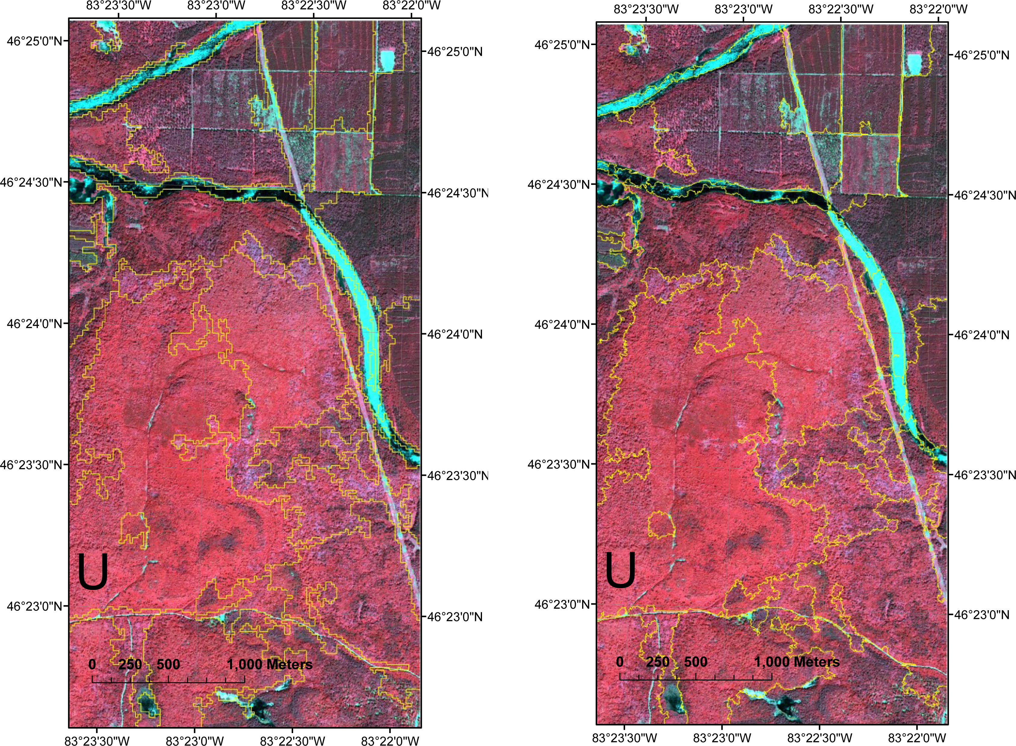
One of the issues with region-growing methods is that they require a set of input parameters to determine the segmentation process. These parameters need to be appropriately determined in order to generate image objects that best represent the features of interest. However, one set of parameters may not be sufficient for the entire area covered by a large remotely sensed image; since it is very likely that a remote sensing image contains objects with different sizes and characteristics. As a result, a single set of parameters often leads to under-segmentation of some parts of the image and over-segmentation of others. A demonstration of this argument is provided in Figure 1. For the segments in Figure 1, a region growing method using on one set of input parameters was applied to a Quickbird image (with a spatial resolution of 2.4 m by 2.4 m) over a forest scene. It is clear that some forest stands were over-segmented, while others were under-segmented.
To optimally segment an image over a large area, we have proposed an adaptive segmentation method for high-spatial resolution imagery [8]. The fundamental idea is to allow the homogeneity criterion to vary from region to region across the whole image, based on the information acquired from a low-spatial resolution representation of the same area. The low-spatial resolution representation can be generated from the original high-spatial resolution imagery or from observations by different sensors. By analyzing a low resolution representation of a study area, coarser features of that area can be more easily identified, which can then be used to determine parameters for use in further analysis of those same areas on the corresponding high-resolution imagery. In this way, over or under segmentation of the high-resolution image can be avoided or minimized. Furthermore, other imagery products, which may not be available in a high-resolution form, such as surface temperature, could in principle, be incorporated for further analysis. However, it was observed that if a segment map determined from a low-resolution image was projected onto its corresponding high-resolution image, the segment boundaries did not align well with the features on the high-resolution image. This misalignment was more severe when data from different sensors were used. The objective of this study was to develop a methodology capable of refining segment boundaries toward multi-scale and adaptive segmentation of high-spatial resolution imagery.
A good physical analogy to our approach to the issue of boundary adjustment is the phenomenon of sand particles settling on a topographical feature. Suppose that a handful of sand is dropped on the top of randomly structured terrain. Under the influence of gravity, these particles would move to areas where the local potential energy is minimal. Based on these same principles, active contouring models were developed to outline objects in computational vision research [6,11–15]. Active contours, also known as snakes, are “energy-minimizing” curves that evolve from their initial positions to fit image features, such as edges and lines, under the influence of image determined forces and external constraints. Active contour methods are classically defined as a curve which is attracted to image features such as edges, lines, or corners [15]. This attraction is quantified by an energy function, which has low values in places on the image which contain those desired features. The energy function also incorporates a term that depends on the shape of the curve and can be used to bias the curve to take on smooth shapes, and a term that depends on user interaction, so that the curve can be interactively pulled toward a desired location [15].
Different energy functions have also been reported in the literature. Some are based on image gradients (the edge-based active contouring models), while others on statistics of the image objects and the background (the region-based active contouring models). The region-based active contouring models do not depend on image gradients and thus are less susceptible to noise and work well for the objects with weak boundaries. The active contour methods for boundary adjustment or boundary detection have been used successfully in the field of medical imaging to detect contrasting regions, such as different tissue types [11,16,17], and in some remote sensing applications as well [10,13,18]. Some drawbacks of utilizing active contour methods include their susceptibility to noise [15,19,20], difficulty with complex images [11,15,20,21], and difficulty in implementing the method when multiple boundaries are present or when boundaries cross [15,21,22]. In addition, the traditional active contour methods utilize a single set of operating parameters which can limit its ability to recognize multi-scale features in an image [18,19].
For our specific situation, we wish to adjust boundaries in a large complex image with multiple boundaries, while trying to maintain the local nature of those boundaries. To achieve this, we adopt the concept of energy-minimization to refining segment boundaries through a new energy function which considers image gradients and regional statistics and also designed an implementation strategy for the adjustment. Our proposed energy function is similar to the traditional active contour energy functions in that the boundary is attracted towards desired features, and is minimized at the desired image locations but is unique in that it does not rely on the curvature of the boundary, incorporates homogeneity, and is explicitly local.
2. Data Used and Low-Spatial Resolution Segments
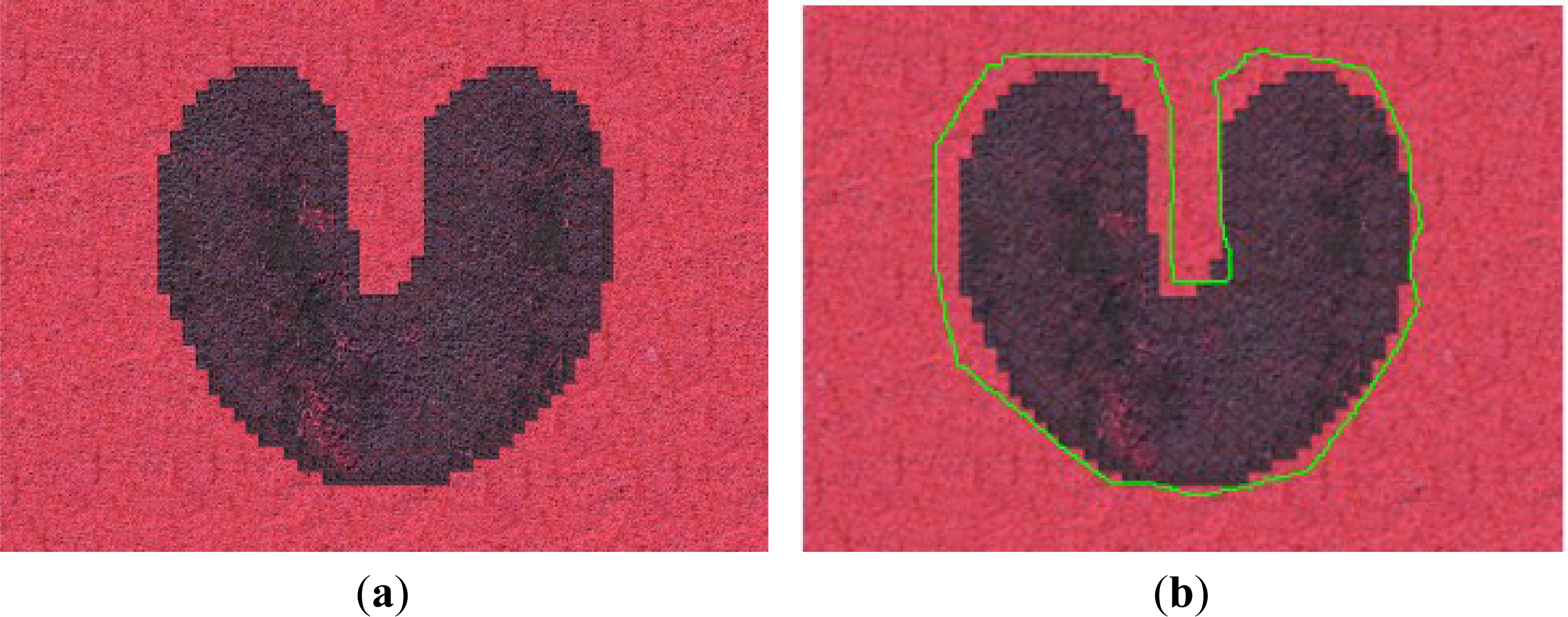
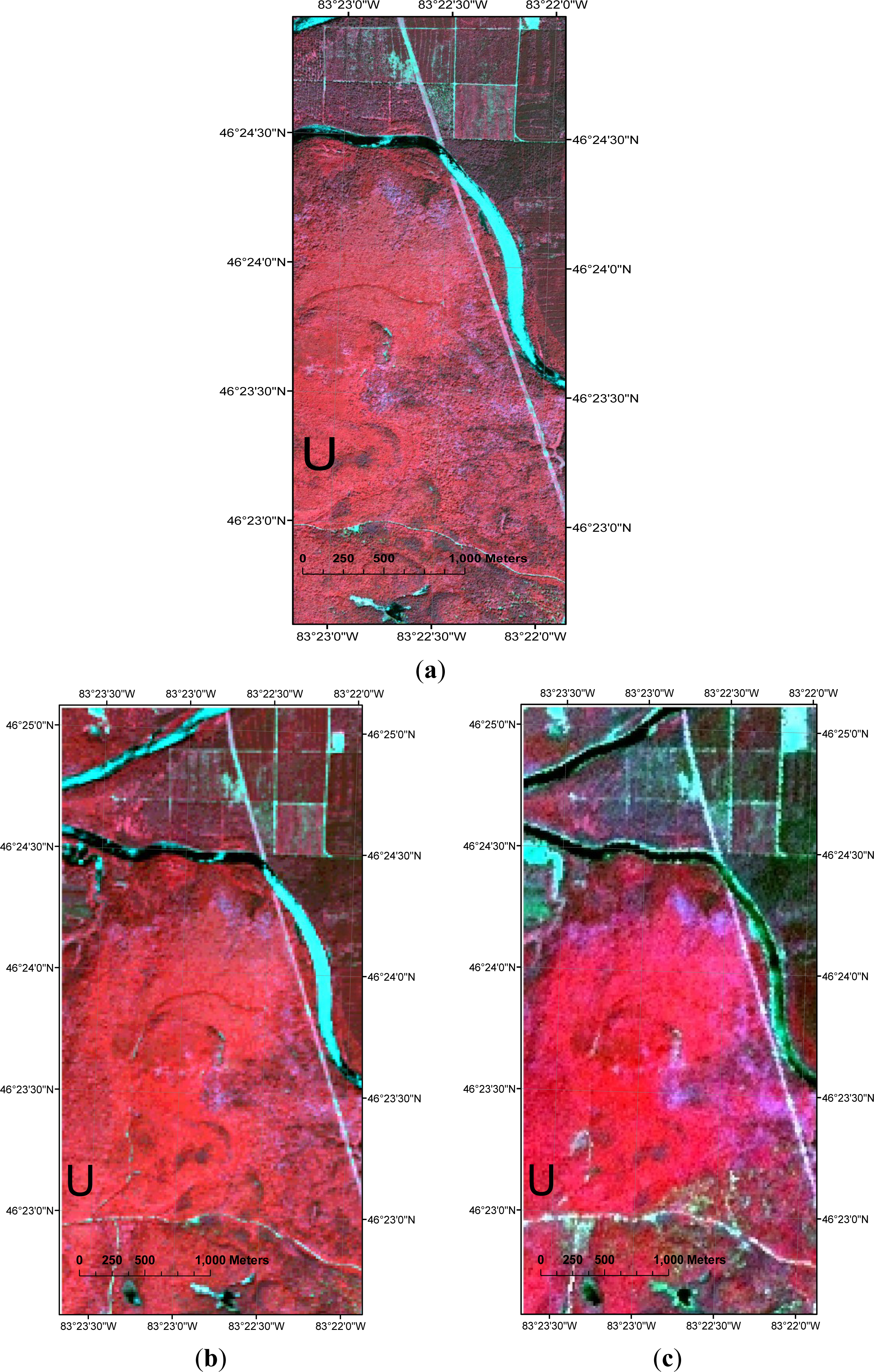
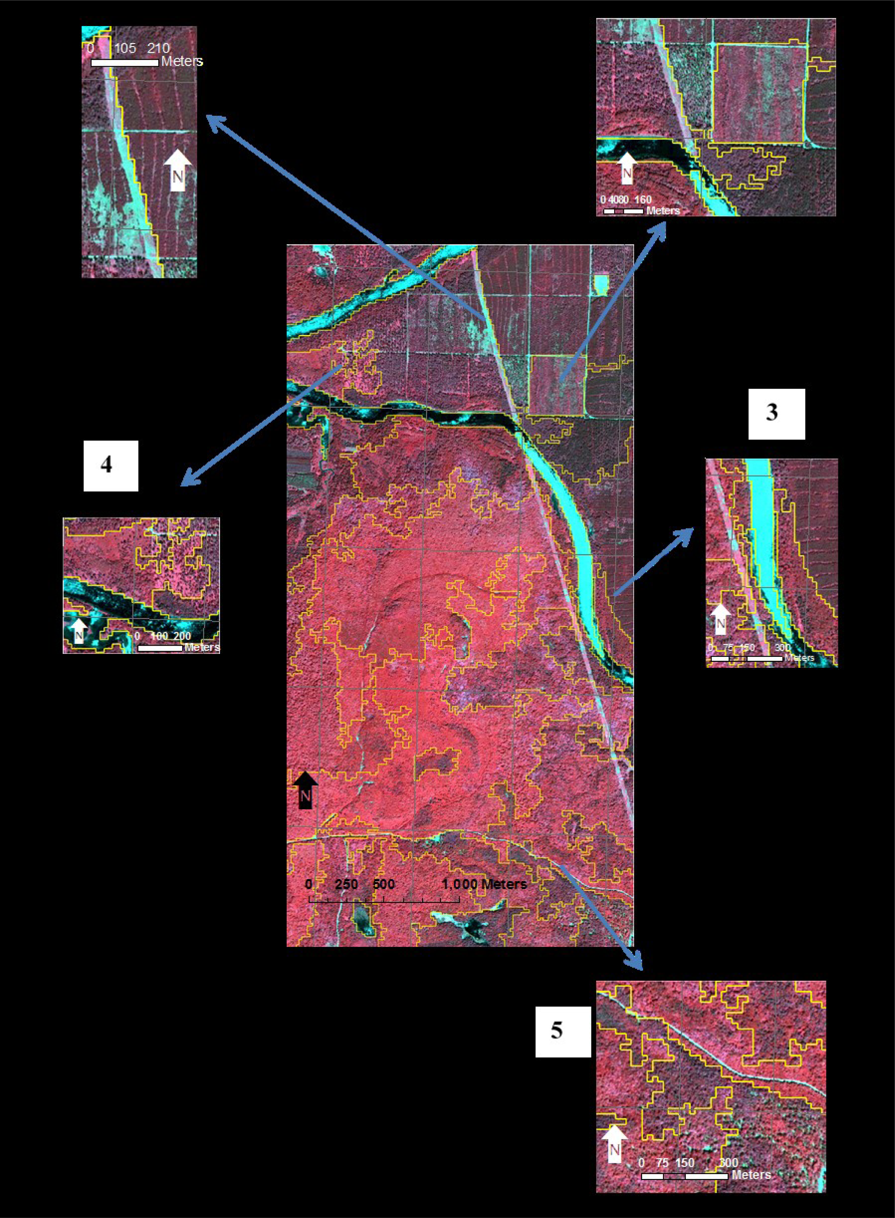
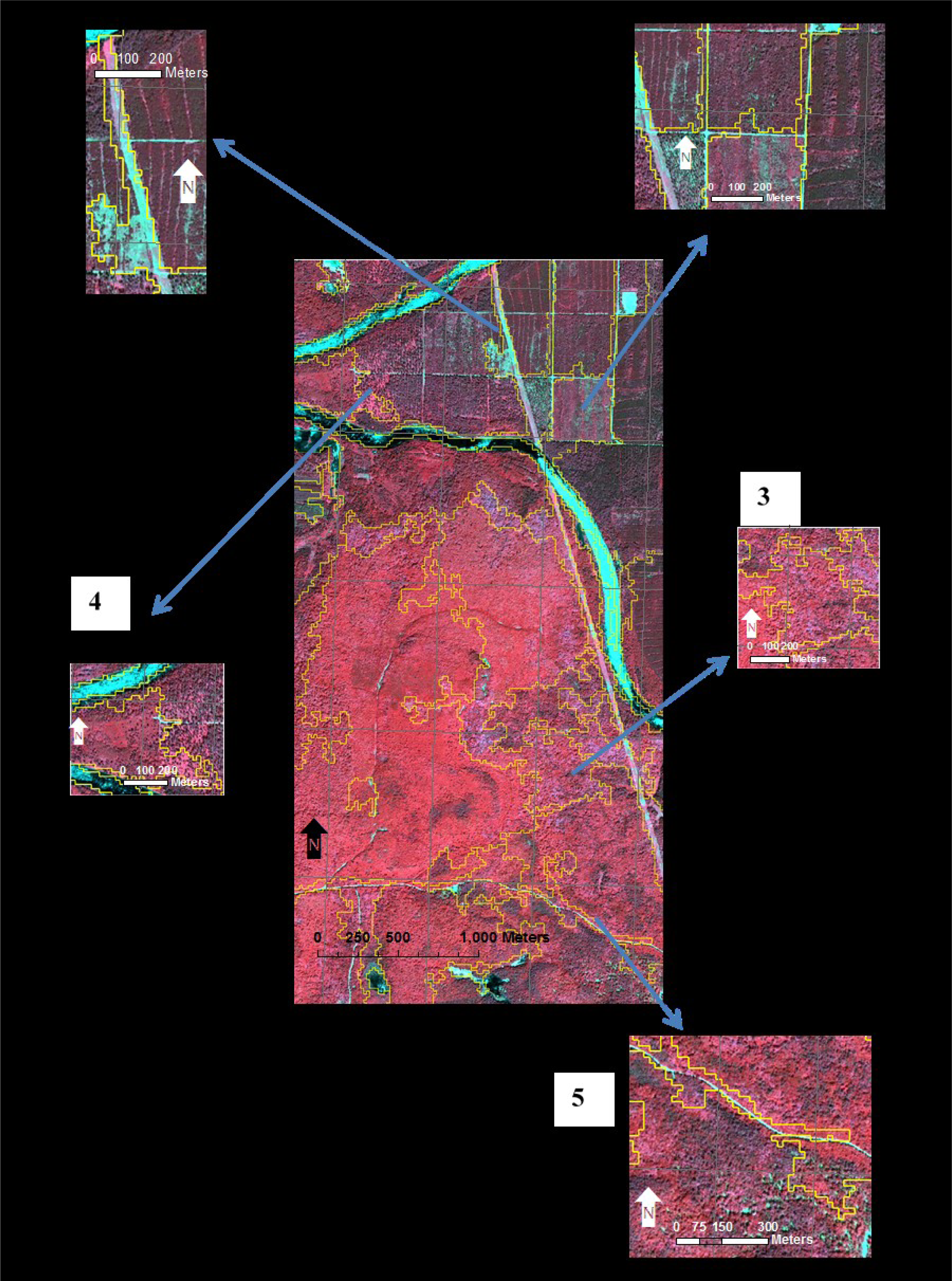
The developed methodology was tested in two phases. In the first phase, testing was conducted on a simple “U-Shaped object”, which is commonly used to test the performance of active contour style methods, with an accompanying boundary which required adjustment, shown in Figure 2. The purpose of this testing was to gain a basic understanding on the performance of the proposed methodology when applied to a simple and widely used image. The geometry of the U-Shaped object was taken from the Image Analysis and Communications Lab at Johns Hopkins University [23], while the accompanying boundary, to be adjusted, was determined by the authors of this paper, inspired by similar shapes which are used in the popular literature. It was noted that there is no single standard or standards for testing, so a shape to suit the needs of this project was created. It should be noted that the images used during this testing phase were “filled in” with information from two different landscapes to create these images. The rationale behind this was to create an object which would mimic the behaviour of structures in a remotely sensed image. In the second phase of testing, tests were conducted on a high-spatial resolution Quickbird [7] image (2.4 m by 2.4 m) over a study area in Ontario, Canada (Figure 3a). Two types of low spatial resolution images were used to provide contextual information to segment the Quickbird image: a resampled Quickbird image (resampled to 15 m by 15 m) and an ASTER (Advanced Spaceborne Thermal Emission and Reflector Radiometer [24]) image at a spatial resolution of 15 m by 15 m. The resampled Quickbird image was created by resampling the high resolution Quickbird image using a bicubic interpolation method, where the outputted pixel was a weighted average of the nearest 4-by-4 neighborhood. The low spatial resolution imagery is shown in Figure 3b,c. Comparing these images, it is noted that features, such as small groups of trees, are discernible on the Quickbird image, but not on the ASTER or resampled Quickbird image. This “washing out” of details on the lower resolution images provides a more generalized view of the larger features of a scene. If a lower resolution forest image was to be segmented, these segments would correspond to forest-stands on the corresponding Quickbird image. When these segments are projected and adjusted onto the Quickbird image, the pixels which these segments encompass can be further analyzed to determine homogeneity parameters for accurate segmentation of the Quickbird image. To segment the low-resolution images, a region-growing program based on the method outlined by Baatz and Schape [25] was used. As an example to illustrate how segments from a low-resolution image correspond to a more generalize view, of the same scene, on a high-resolution image, and how these projected segments do not match well to the features on the corresponding high-resolution image, the segments obtained from the resampled Quickbird image and ASTER image are projected onto the corresponding Quickbird image in Figures 4 and 5. As expected, the segments determined from the ASTER and the resampled Quickbird images, called the projected segments hereafter, encompassed larger features on the Quickbird image, and also do not match well to the features on the Quickbird image.
3. Methodology
3.1. The Energy Function for Boundary Adjustment
The energy function given in Equation (1) was designed in such a way that the following two goals were achieved: the adjusted boundaries were to be aligned well with the image features, such as edges, and additionally, the within-segment homogeneity and between-segment heterogeneity was maximized. This is the objective of any segmentation or adjustment method, which is why it is reflected here. Equation (1) achieves these goals by maximizing within-segment homogeneity and between-segment heterogeneity by determining configurations which result in lower variance and rewarding configurations where edges are better represented by weighing those configurations through further reductions in the energy function.
In Equation (1) Ei,j is the energy at the pixel (i,j) to which the initial boundary could possibly move; N is the number of segments; Mk is the number of pixels in the segment k; B is the number of bands in the image; xk,l,m is the digital number (intensity) of the pixel l in segment k for band m; μk,m is the mean value of the digital numbers for all pixels in segment l, for band m; yij is the value of pixel (i,j) in the image gradient, for a particular adjustment scenario (described further in Section 3.2.2), and ymax is the maximum value in the image gradient for the entire image; and w is a weighting factor. In principle, w can take any positive value. Based on our experiments, when the value of w was up to 3–4, regional statistics had a limited effect on the energy function. In this study, to balance the contribution of image features and regional statistics to the calculated energy, w was fixed to 1. The effect of w on the boundary adjustments will be further analysed in the discussion and conclusions section. Initial segment boundaries were adjusted iteratively to new locations until a configuration was reached where E was at a local minimum within the pre-determined local neighbourhood.
3.2. Boundary Adjustment
Given a high-spatial resolution image and initial segments obtained from a low-spatial resolution representation of the same scene, our method adjusted the segment boundaries by minimizing the energy function in Equation (1) according to the following four phases. In the first phase, called “Edge Mapping”, the gradient (edge) image was created. In the second phase, called “Adjustment Calculation”, for each initial boundary location, all possible adjustments were determined and ranked according to the energy function in Equation (1) and the best adjustment scenario, in terms of the energy minimization, was recommended. In the third phase, called “Adjustment Ranking and Execution” the recommended adjustments in Phase 2 were ranked and executed, locally, in order of energy reduction. In the fourth and final phase called “Termination”, oscillating adjustments and the termination criterion were checked. If the termination criterion was not met, Phases 2–4 were repeated. In the following sections, we will describe these phases.
3.2.1. Phase 1: Edge Mapping
To generate a gradient component of the high spatial resolution image of interest, we implemented a canny edge detection algorithm [26] and applied it to the intensity component (grey-scale) of the test image for each band m. With the implemented canny method, a Gaussian filter was first used to smooth the intensity image. The magnitude and the orientation of the gradient were then calculated using the Sobel templates. Finally, non-maxima suppression was used to remove any pixel that was not considered to be an edge. It should be noted, however, that the resulting image was not binary; no threshold value was used. The resulting gradient images consisted of a range of values depending on the strength of that particular edge pixel. These images were then combined and averaged together to create a final gradient map, which was used to calculate the energy based on Equation (1) in Phase 2.
3.2.2. Phase 2: Adjustment Calculation
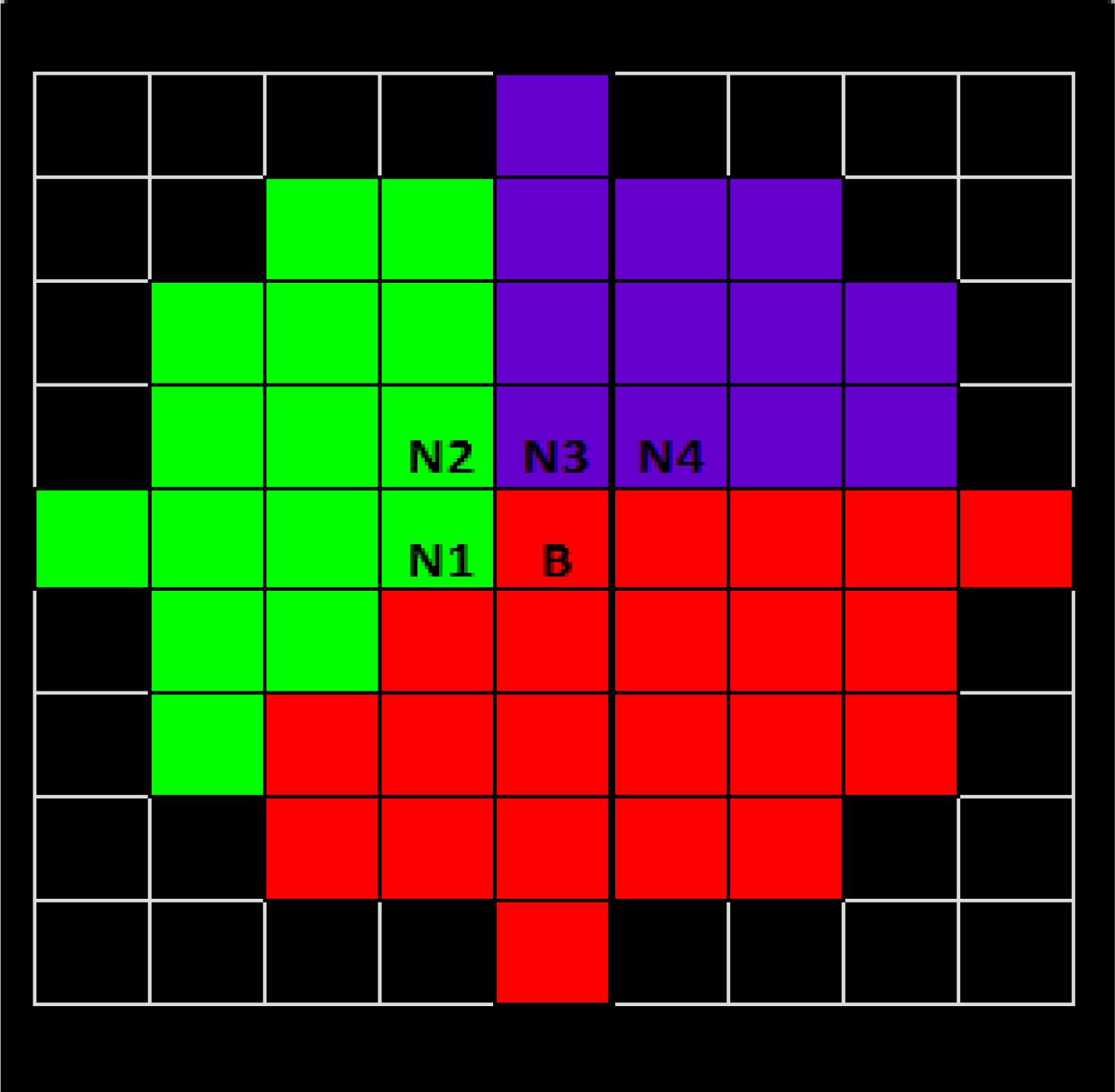
The objective of this phase was to determine the possible movements of each boundary pixel. To do this, a circular buffer was projected around each candidate pixel. The candidate pixel belonged to the border of a segment called the base segment. The buffer encompassing the candidate pixel may often contain portions of the base segment and other segments. As an example in Figure 6 there are three different segments within the buffer around the candidate pixel B. For the base segment, there were six scenarios where its boundary could move from the candidate pixel B.
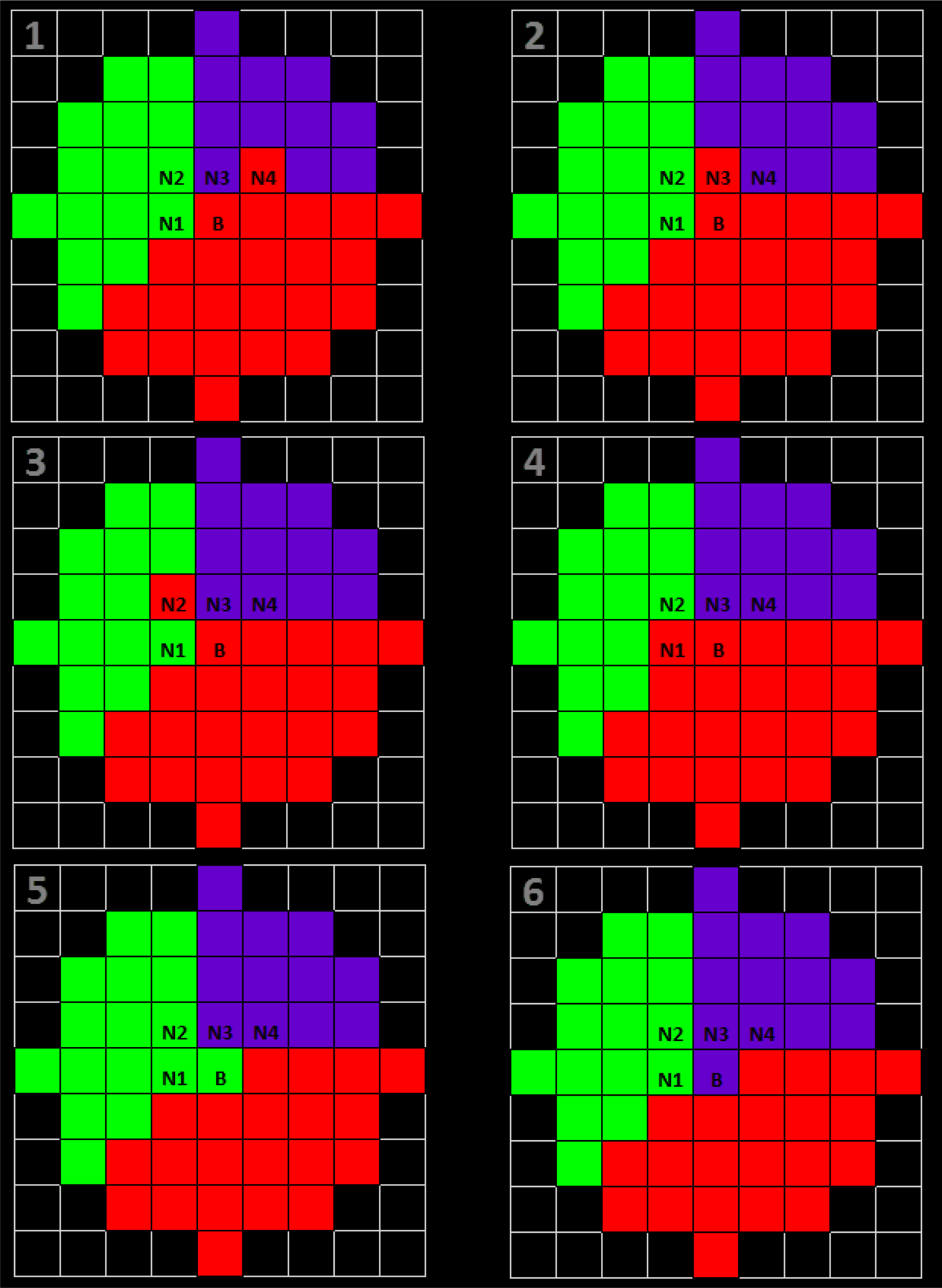
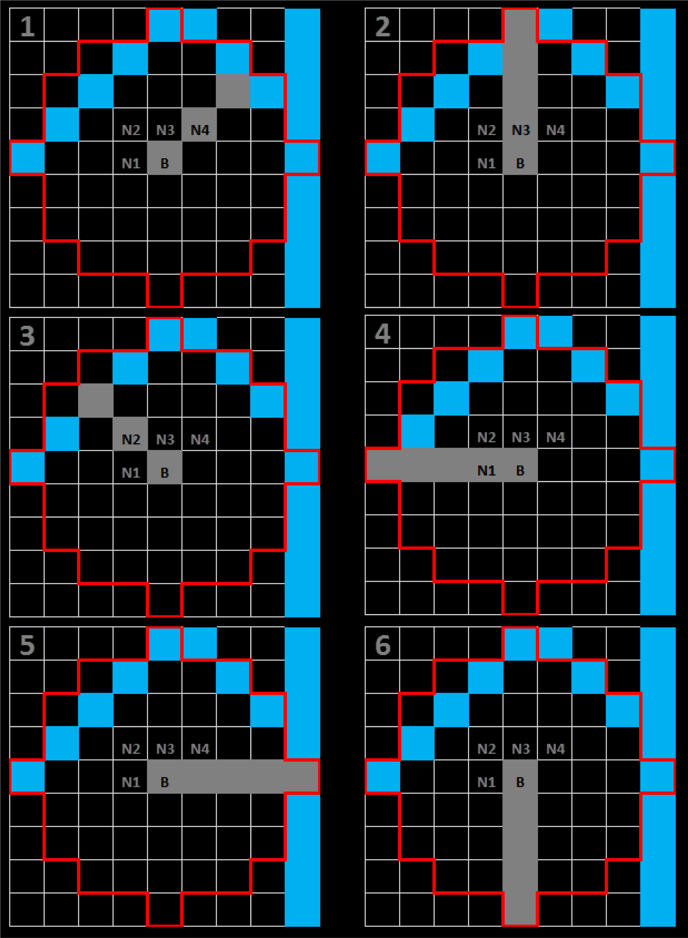
As shown in Figure 7, the base segment could spread to a candidate pixel from one of the neighbours which could belong to other segments (Cases 1, 2, 3 and 4) or it could be shrunk by losing the candidate pixel to either of the other two segments (Cases 5 and 6). The energy function defined in Equation (1) was calculated for each of these six possible adjustment cases and the original setting (Figure 7) with pixel (i, j) being at N4, N3, N2, N1, B, and B, respectively.
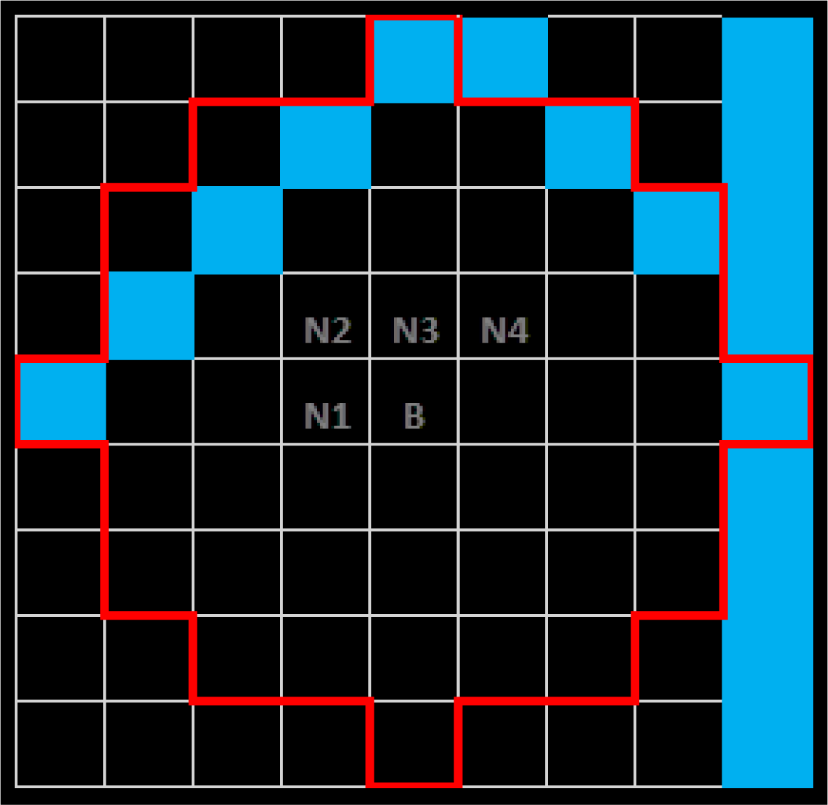
To illustrate how to calculate the edge terms in Equation (1), Figure 8 represents the locations of the edge pixels in this buffer. The blue squares represent edge pixels, and the thin red lines represent the boundaries of the buffer. These boundaries are identical to the boundaries of the buffer shown in Figures 6 and 7. For each of the possible adjustment scenarios in Figure 7, a corresponding edge searching scheme was performed to determine the maximum edge magnitude, for that particular adjustment. As shown in Figure 9, for each potential adjustment scenario, pixels were checked along the direction of the adjustment (to the end of the buffer, illustrated by the gray pixels), and the maximum edge magnitude (yij) in that direction was selected for that particular adjustment. The adjustment scenario which provided the lowest energy was chosen as the recommended adjustment of the base segment at the candidate pixel. If none of the possible adjustments resulted in a lower energy, when compared to its present configuration, no adjustment was recommended. It should be stressed that no actual adjustments were performed in this phase. This process was repeated for all boundary pixels.
3.2.3. Phase 3: Adjustment Ranking and Execution
In this phase, the potential adjustments obtained in Phase 2 were ranked. This was carried out by first projecting a grid onto the high spatial resolution image overlaid with the initial segment boundaries. An illustration of the grids is shown in Figure 10. The recommended adjustments were ranked within each grid based on their minimization of the energy function from their previous configurations. The adjustment resulting in the maximum energy reduction, within that grid, was executed first followed by other adjustments based on their ranking of energy reduction. By doing so, adjustments were only affected by local features, and were carried out in a manner which rewarded the significance of the adjustment. Performing adjustments utilizing a grid was also advantageous because it produced groupings which are ideal for parallel computations. It is worth mentioning that oscillating adjustments were observed for some boundary pixels. An oscillating adjustment occurred when a boundary pixel was adjusted in one iteration, but was adjusted back to its previous positions on the next iteration; and this behaviour was repeated for subsequent iterations. This pixel oscillation was found to prevent the termination criteria from being met. To compensate for this, all adjustments were tracked and if a pixel was identified to be oscillating, further adjustments were not allowed for that pixel.
3.2.4. Phase 4: Termination
The termination criterion was checked in this phase. The termination criterion was defined as the point when the number of adjustments, per-iteration, reached below a user specified level or zero. Also, termination of the algorithm was carried out if the maximum number of iterations, specified by the user, was reached. If the termination criterion was not met, Phases 2–4 were performed again.
3.3. Evaluation of Adjustments
3.3.1. Quantitative Evaluation of Adjustments
In order to quantify the performance of the proposed methodology, two strategies were used. The first was a simple comparison of changes in homogeneity of the segments, before and after adjustment. An increase in homogeneity as measured via a reduction in the standard deviation, after adjustment would indicate that the proposed method is working as designed. The second strategy used to quantify the performance of the proposed methodology was a popular technique called F-measure, described by Estrada and Jepson [27] was used. In order to determine the F-measure of a segmentation result, the precision and recall of that result needs to be calculated. Mathematically, precision and recall are defined in Equations (2) and (3), respectively. Given a segmentation map generated through a segmentation algorithm (called from here on in the reference segment map) Sreference, and a target segmentation map, Starget, created through human interpretation, precision is defined as the proportion of boundary pixels in Sreference for which we can find a matching boundary pixel in Starget.
In order to determine how pixels from either the target or source map match to one another, a matching algorithm also described by Estrada and Jepson [27] was used. For each boundary pixel P = (Xp,Yp) to be matched, a circular window of a radius, r, centered at (Xp,Yp), any boundary pixels, from the other map, within this window are potential matches for P. A boundary pixel Q within the search window is a suitable match for P if the following conditions are satisfied:
- (1)
There are no other boundary pixels in Sreference between P and Q (no intervening contours constraint).
- (2)
The reference pixel that is closets to Q and the source pixel P being matched to Q must be on the same side of the target boundary Q (same side constraint).
Once precision and recall are calculated, F-measure, which is a harmonic average of the two, can be calculated by:
3.3.2. Qualitative Evaluation of Adjustments
Adjustments were also evaluated in terms of a three-level quality classification scheme determined by user input. Through this classification scheme, adjusted results were either classified as being of high, average or lower quality based on the opinions of independent evaluators. During the evaluation process, an evaluator would be presented with 10 sets of images, consisting of an original image and its adjusted result. The evaluator would then rank each adjusted result. This qualitative evaluation provides an alternative to the quantitative approach, which is based on human perceptions and what people would naturally consider quality.
4. Results
Using the algorithm described above, we adjusted the segment boundaries shown in Figures 2b, 4, and 5. A 5 by 5 Gaussian filter was used to smooth the images as part of an edge detection method (Phase 1) and the results are shown in Figures 11 and 12. A buffer with a radius of 10 pixels was used in Phase 2 to determine all of the possible adjustment scenarios for each of the initial boundary locations. A grid size of 20 by 20 pixels was used in Phase 3 to rank the potential adjustments and the termination criterion was set when adjustments reached below three adjustments per iteration, with the maximum number of iterations limited to 200. The selection of these parameters will be discussed later. The final adjusted-segments are shown in Figures 13 and 15. For Figure 13, it would appear that the test boundaries have been successfully matched to the features of the U-Shaped object. For Figures 14 and 15, compared with the original projected boundaries, the adjusted boundaries are smoother and align well with image features. To clearly show the difference between them, several close-up images are shown in Figures 16 and 17. For these close-up areas the initial projected segments can clearly be seen to not match the boundaries of the features in the image. However, after adjustment, those same segments show improvements in both their location and neatness, when compared against those same image features. These adjusted boundaries are very close to easily identified edges and encompass easily identifiable homogeneous areas. In addition, as expected, after the adjustment, segments were found to be more homogeneous, demonstrated by the decrease in the average standard deviation values, determined from the red, green and near-infrared bands from the adjusted-segmented Quickbird image. When the average standard deviation is calculated and compared, based on all segments, before and after adjustment shown in Table 1A,B,C, a decrease in the standard deviation is observed, indicating improved homogeneity for all test images. When examining results from the Ontario test area, these changes were more pronounced with segments determined from the resampled Quickbird image. Adjustments performed on segments determined from the resampled Quickbird image, for the majority of tests, outperformed segments determined from the ASTER image, both in terms of visual inspection and in measured changes towards increased homogeneity.
The second quantitative analysis method, in the form of F-measure, was applied to the adjusted segment maps shown in Figures 13, 16, and 17, using a window of radiuses between 0–5 pixels, which encompasses standard window distances for images of these sizes [27–29]. Those results are summarized in Table 2. When examining Table 2, it is noted that as the window size to match pixels increases so does the F-measure values. Furthermore, it was noted that all adjustments resulted in improved F-measure values, and were performing either at, or above, a threshold of 0.58–0.66 which corresponds to F-measure values generated by the best results from widely used image segmentation and adjustment algorithms [27–29], and in some cases, performing at the level between 0.79–0.84 which is generated from human determined segmentation or adjustment maps which are compared to one another. These results indicate that the proposed method is functioning as designed and is producing adjustments which match closely to those which would be created by other methodologies or human perceptions.
As a final form of evaluation, adjusted segmentation results were classified through a three-level quality classification scheme determined by user input. Through this classification scheme, adjusted results were either classified as being of high, average or lower quality. When examining quality classification results from Figures 16 and 17, for the resampled Quickbird image (Figure 16), areas 2 and 5 were deemed to be of lower quality, areas 3 and 4 were of average quality, and area 1 of high quality. From the ASTER image results (Figure 17), areas 2 and 3 were lower quality, areas 4 and 5 were of average quality, and area 1 of high quality. These results tied in with better overall homogeneity changes, and better overall F-measure values imply that the adjustment method may perform better on segments determined from a resampled Quickbird image, compared to segments determined from an ASTER image, of the same area.
5. Discussion and Conclusions
When examining the results of the proposed adjustment methodology, we first considered the U-Shaped test image. Upon visual inspection it can be clearly seen that the test boundary has been significantly adjusted, and the adjusted boundary matches well to the U-Shaped objects features. From the first quantitative measure of improved homogeneity, as measured by a decrease in standard deviation, averaged from all segments, and after adjustment, it is implied that the adjustment methodology was working as designed. Further quantitative analysis in the form F-measure also supports this with high F-measure values. These visual and quantitative results indicate that the proposed adjustment methodology is functioning as designed. For boundary adjustment or segmentation methods whose performance is measured through F-measure values, it is generally agreed upon that segmentation or adjustment results which produce F-measure values between 0.79 and 0.84 as well as above are comparable to those generated when human generated maps are compared to one another [28,29]. According to these F-measure results, testing of the U-Shaped object indicates that our proposed methodology is generating results which could be comparable to other methods and those generated by human perceptions.
When examining results from the ASTER or resampled Quickbird image, we considered the size and complexity of each test image. Each test image is fairly large (1934 by 967 pixels), each containing over 55 individual segments comprising over 15,000 boundary pixels. Additionally, the image is complex, containing many different types of terrain, which adds value to our testing. Related to this, due to the size and complexity of the test images, it was deemed unreasonable to create a manually determined segment map for all of the adjusted boundaries for comparison purposes. An example of a manually determined segment map is shown in Figure 18.
Ideally, we would manually adjust all of the segment boundaries to generate reference segments, to act as references for quantitative evaluation. Instead, individual test areas for further examination were chosen, and independent evaluators from our group and from a conference were allowed to examine our results. These evaluators helped to create reference maps for the test areas highlighted in Figures 16 and 17. To create these reference maps, the evaluators were presented with a segmentation map, before adjustment, and were then instructed to draw out where they believe those segments should be, on the image. This was all done with the ENVI 5.0 software suite. The resulting segment map constituted the reference map used to determine the F-measure score. These evaluators also aided in ranking those adjustments based on the quality criteria described in Section 3.3.2. By the initial quantitative measure, improved homogeneity as measured through decreases in standard deviation values of the segments, after adjustment, supports our assertion that our method was successfully adjusting results. When analysis using F-measure values was conducted, it was noted that even with a window of 2 pixels, adjusted segments, from the selected test areas, produced F-measure values which were improvements from their original scores and were close to or at the levels of those produced by other methodologies and, in the case of test area 1, for both the ASTER and resampled Quickbird image, values which are comparable to those generated strictly by human perceptions. As a point of note, when comparing results qualitative analysis values to their corresponding F-measure values, it was noted that results which were classified as being of low quality still yielded F-measure values which were considered “good” or “acceptable” from the literature. Again, these results indicate that the proposed methodology is working as designed and is performing as well as, if not better than, other methodologies. Finally, it was noted that through all quality classification approaches, the adjustment method performed better on segments determined from the resampled Quickbird image, compared to segments determined from the ASTER image, of the same area.
One algorithmic consideration for the proposed method regards the choice of buffer radius. For initial testing and evaluation, the radius was chosen by considering the resolution of the image, the image size and trial and error. However, factors such as signal to noise ratio, homogeneity parameters, and an ultimate rationale behind choosing a buffer size were not used. In future work, a rational method should be established which determines the buffer size by taking into consideration image size, image resolution, signal to noise ratio, and homogeneity parameters. Another aspect which should be explored is the progressive adjustment of the buffer size. In preliminary testing of the concept, it was found that some results were improved by progressively increasing the buffer radius until it reached a predetermined length. Further exploration and development of this should be conducted and a more formal approach to applying the concept of a progressive buffer size should be developed. In this vein, another consideration was the choice of grid size. In this study, the grid size was chosen by considering the buffer size, and the size of the image. However, like buffer size a rational method, which takes into account those same factors, should be used in its determination. In line with that, it was acknowledged that if too large a grid size was selected, it would defeat the purpose of the grid. The same can be concluded about selecting a gird that was too small; the ranking scheme would then become irrelevant.
An additional algorithmic consideration concerns the adjustments of pixels which lie on the boundaries of the adjustment grid. Pixels which lie on the boarder of a grid square could be adjusted several times when in principle they should be adjusted only once. An acceptable solution to address this issue has not yet been presented and it is not known how this issue affects quality.
With regards to the incorporation of edge information, determining the weight of edge information, and noise considerations from the edge map requires investigation. For the purposes of this study, the weighting of the edge information was set to 1 in the energy function (Equation (1)), although a limited number of tests were also conducted in order to explore the effects of various edge weights. Tests where the weight was set to 0, illustrated the importance of incorporating edge information. Figure 19 shows the difference in adjustments when edge information is incorporated and when it is not. Using edge information was almost always beneficial to adjustments. Other tests showed that as the edge weight was increased to 2 it had a limited effect on adjustments until it reached a transition point around 3–4 where the edge information dominated the energy function and produced poorer results.
Regardless of the edge weight, when edge information was incorporated, it was observed that noisy edge maps could affect results by promoting noise driven adjustments as opposed to ones driven by actual edges. How the signal to noise ratio relates to the quality of results is not known and requires further investigation. More advanced, multi-scale or alternative approaches to producing edge maps should be investigated in further developments to address these concerns.
The elimination of the oscillating behaviour in pixel adjustments presents another algorithmic consideration. The point in which the algorithm determines when to be sensitive to the oscillating behaviour was determined through recording the number of adjustments per iteration and then checking if those adjustments were displaying asymptotic behaviour. If it was found that the adjustments had become asymptotic as the program was allowed to become sensitive to recording and eliminating the oscillating behaviour. In future versions, a more advanced method to identify this behaviour should be explored, to allow the method to become more independent of user input, and more reliable.
In summary, the presented boundary adjustment method was successful in adjusting the boundaries of a segmentation map that was determined from a low resolution resampled Quickbird image or ASTER image, projected onto its corresponding Quickbird image. It was found that the resulting adjusted-segments had morphed into a configuration where the undesirable boundaries had been adjusted and the overall homogeneity of the segments in that image had been improved. The adjusted-segment map matched closely to the features from the Quickbird image. This method is innovative in two aspects. The first innovative aspect was its utilization of a local buffer to determine single pixel adjustments based on minimizing an energy function, within a buffer. The second was the manner in which those adjustments were carried out, through local ranking, based on the greatest changes towards homogeneity, and the execution of those adjustments through the use of a grid which aided in grouping, ranking, and localizing those adjustments. The energy function is new as well; it integrated the energy functions used in the edge-based and region-based active contouring models. The work presented here can be used as a strong basis to develop/implement multi-scale and adaptive remote sensing segmentation techniques.
Acknowledgments
The authors are grateful for financial support provided by the Natural Sciences and Engineering Research Council (NSERC) of Canada. The ASTER data product was obtained through the online Data Pool at the NASA Land Processes Distributed Active Archive Center (LP DAAC), USGS/Earth Resources Observation and Science (EROS) Center, Sioux Falls, South Dakota.
Author Contributions
Aaron Judah had the original idea for the study and, with all co-authors carried out the design. Aaron Judah, and Baoxin Hu, were responsible for recruitment and follow-up of study participants. Aaron Judah, and Baoxin Hu was responsible for data cleaning and Aaron Judah carried out the analyses. Aaron Judah, Baoxin Hu, and Jain-guo Wang drafted the manuscript, which was revised by all authors. All authors read and approved the final manuscript.
Conflicts of Interest
The authors declare no conflict of interest.
References
- Benz, U.C.; Hofmann, P.; Willhauck, G.; Lingenfelder, I.; Heynen, M. Multi-resolution, object-oriented fuzzy analysis of remote sensing data for GIS-ready information. ISPRS J. Photogramm. Remote Sens 2004, 58, 239–258. [Google Scholar]
- Blaschke, T.; Strobl, J. What’s wrong with pixels? Some recent developments interfacing remote sensing and GIS. GeoBIT/GIS 2001, 6, 12–17. [Google Scholar]
- Wu, Q.; An, J.; Lin, B. A texture segmentation algorithm based on PCA and global minimization active contour model for aerial insulator images. IEEE J. Sel. Top. Appl. Earth Obs. Remote Sens 2012, 5, 1509–1518. [Google Scholar]
- Burnett, C; Blaschke, T. A multi-scale segmentation/object relationship modelling methodology for landscape analysis. Ecol. Model 2003, 168, 233–249. [Google Scholar]
- Blaschke, T.; Burnett, C.; Pekkarinen, A. New Contextual Approaches Using Image Segmentation for Object-Based Classification. In Remote Sensing Image Analysis: Including the Spatial Domain; De Meer, F., de Jong, S., Eds.; Kluver Academic Publishers: Dordrecht, The Netherland, 2004; pp. 211–236. [Google Scholar]
- Chan, T.; Sandberg, B; Vese, L. Active contours without edges for vector-valued images. J. Vis. Commun. Image Represent 2001, 11, 130–141. [Google Scholar]
- Core Imagery Products Guide. Available online: http://www.digitalglobe.com/sites/default/files/DigitalGlobe_Core_Imagery_Products_Guide_0.pdf (accessed on 17 April 2014).
- Hu, B.; Li, J.; Jing, J.; Judah, A. Improving the efficiency and accuracy of individual tree crown delineation from high-density LiDAR data. Int. J. Appl. Earth Obs. Geoinf 2014, 26, 145–155. [Google Scholar]
- Dey, V.; Zhang, Y.; Zhoug, M. A. Review on Image Segmentation Techniques with Remote Sensing Perspective. Proceedings of ISPRS TC VII Symposium—100 Years, Vienna, Austria, 5–7 July 2010; Wagner, W., Székely, B., Eds.; ISPRS: Vienna, Austria, 2010. [Google Scholar]
- Xu, C.; Prince, J.L. Gradient Vector Flow: A New External Force for Snakes. Proceedings of the 1997 IEEE Computer Society Conference on Computer Vision and Pattern Recognition, San Juan, Puerto Rico, 17–19 Jun 1997; pp. 66–71.
- Chan, T.; Vese, L.A. Active Contour and Segmentation Models Using Geometric PDE’s for Medical Imaging. In Geometric Methods in Bio-medical Image Processing; Springer: Berlin, Germany, 2002; pp. 63–75. [Google Scholar]
- Cremers, D.; Rousson, M.; Deriche, R. A review of statistical approaches to level set segmentation: Integrating color, texture, motion and shape. Int. J. Comput. Vis 2007, 72, 195–215. [Google Scholar]
- Chang, H-H.; Daniel, V.; Chu, W. Active shape modeling with electric flows, visualization and computer graphics. IEEE Trans. Vis. Comput. Gr 2010, 16, 854–869. [Google Scholar]
- Kass, M.; Witkin, A.; Terzopoulos, D. Snakes: Active contour models. Int. J. Comput. Vis 1988, 1, 321–331. [Google Scholar]
- Mishra, A.K.; Fieguth, P.W.; Clausi, D.A. Decoupled active contour (DAC) for boundary detection. IEEE Trans. Pattern Anal. Mach. Intell 2011, 33, 310–324. [Google Scholar]
- Zhang, K.H.; Song, H.H.; Zhang, L. Active contours driven by local image fitting energy. Pattern Recognit 2010, 43, 1199–1206. [Google Scholar]
- Zhang, Y.; Matuszewski, B.J.; Shark, L.-K; Moore, C.J. Medical Image Segmentation Using New Hybrid Level-Set Method. Proceedings of the Fifth International Conference BioMedical Visualization, 2008 (MEDIVIS ’08), London, UK, 9–11 July, 2008; pp. 71–76.
- Thomas, N.; Hendrix, C.; Congalton, R.G. A comparison of urban mapping methods using high-resolution digital imagery. Photogramm. Eng. Remote Sens 2003, 69, 963–972. [Google Scholar]
- Hu, B.; Judah, A. Multi-scale and adaptive segmentation of high-spatial resolution imagery. Remote Sens. Environ 2013. submitted.. [Google Scholar]
- Yu, Q.; Gong, P.; Chinton, N.; Biging, G.; Kelly, M.; Schirokauer, D. Object based detailed vegetation classification with airborne high spatial resolution remote sensing imagery. Photogramm. Eng. Remote Sens 2006, 72, 799–811. [Google Scholar]
- Nakhmani, A.; Tannenbaum, A. Self-crossing detection and location for parametric active contours. IEEE Trans. Image Process 2012, 21, 3150–3156. [Google Scholar]
- Tilton, J; Lawrence, W. Interactive Analysis of Hierarchical Image Segmentation. Proceedings of the IEEE 2000 International Geoscience and Remote Sensing Symposium, 2000 (IGARSS 2000), Honolulu, HI, USA, 24–28 July 2000.
- Yuan, J.; Li, P.; Wen, Y.; Xu, Y. Level set segmentation of intensity inhomogeneous images based on local linear approximation of difference image. Image Process. IET 2012, 6, 473–482. [Google Scholar]
- ASTER User Handbook, Version 2. Available online: http://www.pancroma.com/downloads/aster_user_guide_v2.pdf (accessed on 17 April 2014).
- Baatz, M.; Schäp, M. Multiresolution Segmentation an Optimization Approach for High Quality Multi-Scale Image Segmentation. In Angewandte Geographische Informations-Verarbeitung XII; Strobl, J., Blaschke, T., Griesebner, G., Eds.; Wichmann Verlag: Karlsruhe, Germany, 2000; pp. 12–23. [Google Scholar]
- Canny, J. A computational approach to edge detection. IEEE Trans. Pattern Anal. Mach. Intell 1986, 8, 679–698. [Google Scholar]
- Estrada, F.J.; Jepson, A.D. Benchmarking image segmentation algorithms. Int. J. Comput. Vis 2009, 85, 167–181. [Google Scholar]
- Arbelaez, P.; Maire, M.; Fowlkes, C.; Malik, J. Contour detection and hierarchical image segmentation. IEEE Trans. Pattern Anal. Mach. Intell 2011, 33, 898–916. [Google Scholar]
- Martin, D.R.; Fowlkes, C.C.; Malik, J. Learning to detect natural image boundaries using local brightness, color and texture cues. IEEE Trans. Pattern Anal. Mach. Intell 2004, 26, 530–549. [Google Scholar]


| (A)
| |||
| Test Boundaries for U-Shaped Object | Average Standard Deviation | ||
| Red | Green | Near-Infrared | |
| Before adjustment | 5.683 | 3.044 | 3.561 |
| After adjustment | 3.983 | 2.914 | 3.390 |
| (B)
| |||
| Initial Segments Determined from Resampled Quickbird | Average Standard Deviation | ||
| Green | Red | Near-Infrared | |
| Before adjustment | 3.326 | 2.255 | 19.544 |
| After adjustment | 2.873 | 1.833 | 16.722 |
| (C)
| |||
| Initial Segments Determined from ASTER | Average Standard Deviation | ||
| Green | Red | Near-Infrared | |
| Before adjustment | 5.412 | 4.592 | 22.367 |
| After adjustment | 4.453 | 3.645 | 17.746 |
| (A) | ||||||
|---|---|---|---|---|---|---|
| F-Measure Determined from Test Areas before Adjustment | Window Size (pixels) | |||||
| R = 0 | R = 1 | R = 2 | R = 3 | R = 4 | R = 5 | |
| ASTER Area 1 | 0.095 | 0.166 | 0.208 | 0.243 | 0.324 | 0.399 |
| ASTER Area 2 | 0.083 | 0.107 | 0.124 | 0.164 | 0.219 | 0.269 |
| ASTER Area 3 | 0.116 | 0.142 | 0.182 | 0.194 | 0.223 | 0.242 |
| ASTER Area 4 | 0.081 | 0.129 | 0.203 | 0.235 | 0.252 | 0.260 |
| ASTER Area 5 | 0.077 | 0.082 | 0.115 | 0.170 | 0.226 | 0.279 |
| Resampled Area 1 | 0.104 | 0.154 | 0.199 | 0.240 | 0.320 | 0.394 |
| Resampled Area 2 | 0.097 | 0.121 | 0.164 | 0.209 | 0.278 | 0.342 |
| Resampled Area 3 | 0.128 | 0.139 | 0.200 | 0.210 | 0.222 | 0.236 |
| Resampled Area 4 | 0.131 | 0.144 | 0.232 | 0.250 | 0.266 | 0.277 |
| Resampled Area 5 | 0.012 | 0.061 | 0.112 | 0.168 | 0.224 | 0.278 |
| (B) | ||||||
|---|---|---|---|---|---|---|
| F-Measure Determined from Test Areas after Adjustment | Window Size (pixels) | |||||
| R = 0 | R = 1 | R = 2 | R = 3 | R = 4 | R = 5 | |
| ASTER Area 1 | 0.543 | 0.719 | 0.859 | 0.882 | 0.895 | 0.895 |
| ASTER Area 2 | 0.352 | 0.452 | 0.509 | 0.571 | 0.595 | 0.604 |
| ASTER Area 3 | 0.332 | 0.496 | 0.520 | 0.553 | 0.637 | 0.656 |
| ASTER Area 4 | 0.405 | 0.517 | 0.581 | 0.672 | 0.721 | 0.742 |
| ASTER Area 5 | 0.355 | 0.491 | 0.547 | 0.578 | 0.604 | 0.625 |
| Resampled Area 1 | 0.564 | 0.739 | 0.854 | 0.862 | 0.876 | 0.883 |
| Resampled Area 2 | 0.421 | 0.579 | 0.672 | 0.707 | 0.743 | 0.768 |
| Resampled Area 3 | 0.388 | 0.410 | 0.573 | 0.599 | 0.636 | 0.674 |
| Resampled Area 4 | 0.547 | 0.612 | 0.664 | 0.715 | 0.761 | 0.792 |
| Resampled Area 5 | 0.374 | 0.467 | 0.549 | 0.567 | 0.594 | 0.620 |
© 2014 by the authors; licensee MDPI, Basel, Switzerland This article is an open access article distributed under the terms and conditions of the Creative Commons Attribution license (http://creativecommons.org/licenses/by/3.0/).
Share and Cite
Judah, A.; Hu, B.; Wang, J. An Algorithm for Boundary Adjustment toward Multi-Scale Adaptive Segmentation of Remotely Sensed Imagery. Remote Sens. 2014, 6, 3583-3610. https://doi.org/10.3390/rs6053583
Judah A, Hu B, Wang J. An Algorithm for Boundary Adjustment toward Multi-Scale Adaptive Segmentation of Remotely Sensed Imagery. Remote Sensing. 2014; 6(5):3583-3610. https://doi.org/10.3390/rs6053583
Chicago/Turabian StyleJudah, Aaron, Baoxin Hu, and Jianguo Wang. 2014. "An Algorithm for Boundary Adjustment toward Multi-Scale Adaptive Segmentation of Remotely Sensed Imagery" Remote Sensing 6, no. 5: 3583-3610. https://doi.org/10.3390/rs6053583
APA StyleJudah, A., Hu, B., & Wang, J. (2014). An Algorithm for Boundary Adjustment toward Multi-Scale Adaptive Segmentation of Remotely Sensed Imagery. Remote Sensing, 6(5), 3583-3610. https://doi.org/10.3390/rs6053583