Global Ecosystem Response Types Derived from the Standardized Precipitation Evapotranspiration Index and FPAR3g Series

Abstract
: Observing trends in global ecosystem dynamics is an important first step, but attributing these trends to climate variability represents a further step in understanding Earth system changes. In the present study, we classified global Ecosystem Response Types (ERTs) based on common spatio-temporal patterns in time-series of Standardized Precipitation Evapotranspiration Index (SPEI) and FPAR3g anomalies (1982–2011) by using an extended Principal Component Analysis. The ERTs represent region specific spatio-temporal patterns of ecosystems responding to drought or ecosystems with decreasing severity in drought events as well as ecosystems where drought was not a dominant factor in a 30-year period. Highest explanatory values in the SPEI12-FPAR3g anomalies and strongest SPEI12-FPAR3g correlations were seen in the ERTs of Australia and South America whereas lowest explanatory value and lowest correlations were observed in Asia and North America. These ERTs complement traditional pixel based methods by enabling the combined assessment of the location, timing, duration, frequency and severity of climatic and vegetation anomalies with the joint assessment of wetting and drying climatic conditions. The ERTs produced here thus have potential in supporting global change studies by mapping reference conditions of long term ecosystem changes.1. Introduction
There is a growing concern about the impacts of global climate change on human and ecological systems [1]. Climate is one of the main determinants of ecosystem composition and functioning [2] which in turn provides a multitude of ecological functions and services that human societies depend upon [3]. Changes have been already documented in patterns of global precipitation, in redistributions of precipitation amounts and in the intensification of the hydrologic cycle leading to increasing heavy rain events or increasing duration of droughts [4,5]. Future projections indicate that observed trends in changing temperature and precipitation patterns will continue, resulting in more frequent and more severe extreme events [5,6].
Complex global systems are able to respond to changing pressures to a certain level [7] whereas reaching the limit of ecosystems adaptive capacity may trigger irreversible processes [8,9]. These changes have already had, and will continue to have, dramatic effects on the productivity, biodiversity and biogeochemistry of terrestrial ecosystems [10]. With warming climate, the geographical border of climatic envelops will shift leading to redistribution of terrestrial ecosystems as floral and faunal components follow the shifting climate. This might lead to extinction of species which in turn might accelerate changes in key ecosystem processes important to the functioning, productivity and sustainability of global ecosystems [11–16]. There are indications that safe boundary limits of many fundamental Earth system processes are being approached [7,9] but we know little about the tipping points in our socio-ecological systems and how fast they might be approaching [17].
Detection of regional [18–22] and global vegetation dynamics [23–26] using remote sensing time-series and linking these to climate [27–32] have already improved the understanding of ecosystem dynamics. However, there are still gaps in information on how ecosystems respond to global climate fluctuations. Methodological challenges in quantifying climate change impacts on ecosystems are still a major issue and there is a need to regularly report observations and results in a way that could lead to rapid recognition, understanding and repeatable monitoring of global environmental problems.
Drought is one of the main climatic drivers of the reduction in Aboveground Net Primary Production [33] and although ecosystems differ in their sensitivity to drought, key ecosystem processes may be hampered in all. Pixel-wise correlation/regression analysis of drought-vegetation cover relationship has been exhaustively studied in the literature. However, this kind of analysis may in some cases result in spurious positive correlation if, e.g., negative anomalies in the SPEI12 and vegetation signal coincide with the non-vegetated period due to, e.g., snow cover (often occurring in the Northern Hemisphere). Furthermore, such an analysis might not indicate drought affected areas if the positive correlations are driven by positive anomalies or if both series express a positive trend thus decreasing drought intensity. Most importantly, a pixel-wise analysis gives information only on the location and strength of the relationship between the vegetation-climate signals but does not inform on the timing, duration, frequency and severity of drought neither on the increase or decrease of this severity. Without such information it is not possible to assess the effect of climatic variations on ecosystems.
In the present study, we classify global ecosystems by analyzing spatio-temporal co-variability of 30-year (1982–2011) vegetation change patterns and climatic fluctuations. Time series of the Standardized Precipitation and Evapotranspiration Index (SPEI) and of the Fraction of Photosynthetically Active Radiation (FPAR3g) were applied in characterizing spatio-temporal co-variability of global ecosystem changes. Ecosystems where the vegetation cover responds in a similar way to climatic fluctuations were grouped into the same Ecosystem Response Types (ERTs). SPEI and FPAR3g temporal profiles were derived for each ERT enhancing the understanding of the timing, duration, frequency and severity of the climatic anomaly and corresponding vegetation response. The derived Ecosystem Response Types were further analyzed in terms of their FPAR3g and SPEI anomalies and dynamics by gradient analysis whereas one- and two-way Anovas were used to test the explanatory power of the ERTs, climate zones, land management classes and their combinations in terms of FPAR3g and SPEI correlations.
2. Data
The gridded global drought dataset Standardized Precipitation-Evapotranspiration Index (SPEI dataset v2.0) was used to address climatic anomalies [34]. Besides the input from precipitation, SPEI also accounts for the possible effects of temperature variability and temperature extremes by implying data on evapotranspiration. Monthly SPEI data covering the time scale of 12 months (SPEI12) from 1982–2011 at a spatial resolution of 0.5° lat/long was used. A timescale of 12 months (or larger) is commonly used to monitor long-lasting dry episodes and therefore consequently is more sensible to detect hydrological drought as compared to smaller shorter timescales that instead target the detection of meteorological and/or agricultural droughts [35].
A long-term global dataset of Fraction of Photosynthetically Active Radiation absorbed by vegetation (FPAR) for monitoring global vegetation dynamics (FPAR3g) [36] was applied to address vegeatation anomalies. FPAR3g is generated as a bimonthly product in a 1/12 degree spatial resolution spanning from July 1981 to December 2011 based on the trained neural network algorithm. The improvements in the recent GIMMS3g NDVI product (superseding the previous GIMMSg) ensuring a spatio-temporal consistent FPAR3g product is primarily related to the use of Bayesian methods with high quality well-calibrated SeaWiFS NDVI data for deriving model AVHRR NDVI calibration parameters [37] (in this issue). The quality of FPAR3g data set have been evaluated through the combined use of field measurements, existing satellite based FPAR3g products and existing Earth System Models permitting the calculation of an overall accuracy assessment of the product [36].
To aid the interpretation of results in how ecosystems reflect global climatic changes, the Köppen climate classification [38] was used. Land use and management on the global scale was addressed by using the Land Use Systems (LUS) maps of the world produced by the United Nations Food and Agricultural Organization [39]. The LUS classification includes several layers as the Global Land Cover dataset (GLC 2000), maps indicating cropping patterns (e.g., dominant crop types), livestock data, major ecosystem types, biophysical resources base layers (e.g., temperature regime, length of growing period, dominant soil units and terrain information) and socio-economic attributes. All classes of the Köppen and the FAO LUS classification were included in the analysis, as the main interest of the study was to compare their explanatory value with the ERTs at the most detailed thematic level.
3. Methods
3.1. Data Pre-Processing
Monthly FPAR3g data was calculated by computing the maximum value of each bi-monthy observation. Since the SPEI12 dataset represents monthly anomalies, these were also calculated for the FPAR3g dataset as:
3.2. Spatio-Temporal Assessment of Combined FPAR3g and SPEI12 Anomalies
Extended Principal Component Analysis (EPCA) was applied to reveal the spatio-temporal co-variability between vegetation vigor and drought anomalies. EPCA is described briefly as follows: Given two matrices N and S, the elements of NT,m are the two-monthly FPAR3g anomalies at T different times and m different spatial cells. The elements of matrix ST,n are the two-monthly SPEI anomalies with the same time domain (T) and at n locations. The difference of the dimension of the spatial locations of the two matrices is due to the different spatial resolution of the FPAR3g and SPEI datasets which do not have to match for an EPCA analysis, where only the matching dimension of the time domain is a prerequisite. The NST,m+n matrix is formed by concatenating matrix N and S forming T time domain at m + n spatial locations. The covariance matrix CT*T is formed from NT,m and ST,n so that:
Then, the eigenvalue decomposition on the covariance matrix C is carried out yielding:
The eigenvectors are calculated as the columns of matrix U a follows:
Each eigenvector includes a spatial pattern of the FPAR3g time-series (NU) in elements 1 m and a spatial pattern of the SPEI time-series (SU) in elements m + 1, …, n. The temporal profiles are computed by projecting matrices N and S onto their own eigenvectors. Thus, the Temporal Profiles of the FPAR3g (NTP) are computed as:
Pixels at different latitudes are assigned different weights in the variance/covariance evaluation process to account for areal distortion. The weight is determined using a cosine rule as follows:
Since the sum of the squares of the singular values in matrix λ is equal to the total squared covariance between all the elements of the SPEI12 and the FPAR3g, each singular value indicates the relative importance of the corresponding spatial modes and subsequent singular values explain the variation after the previous singular value has been accounted for. Using all dimensions (equal the number of input bands) would introduce unnecessary noise in the analysis as the first few dimensions summarize most of the co-variation in the datasets. The singular values therefore were plotted similarly to a scree-plot which, when read left-to-right across the abscissa can show a clear separation in fraction of total covariance. Only the first 15 combined PCA dimensions were selected (30% of the total covariance explained) for the further analysis as after this dimension the fraction of total covariance substantially decreased. The combined spatial patterns of the co-varying SPEI and FPAR3g patterns for these 15 dimensions were calculated by correlating the temporal profiles of the SPEI (STP) with the FPAR3g time series over each pixel and writing the correlation coefficients as a 15-band image.
3.3. Classification of Ecosystem Response Types
The inter-annual variation of vegetation canopy reflectance is subject to factors that are not related to ecosystem structure or function but to residual effects of satellite drift, calibration uncertainties, sensor differences or atmospheric effects [40]. These effects introduce variability in the satellite data that are artifacts and are not due to real changes in the surface reflectance or derived vegetation metric. Therefore, spatial autocorrelation was calculated for each of the first 15 dimensions of the combined spatial patterns using the Getis-Ord Gi* statistics. The resulting z-scores indicate where features with either high or low values cluster spatially. We selected the eight neighbors rule within a moving window that ensures that the resulting Gi* values are normally distributed and considered the centre of the moving window as well, which is more appropriate for use in remote sensing [41]. For a detailed description see [21].
The spatial autocorrelation values were submitted to an ISODATA cluster analysis. To maintain variability due to region-specific climatic, ecosystem, land cover and land use conditions, the cluster analysis was run for each continent separately. First the classification was run with five iterations and subsequently we increased the number of iterations from five up to 100. The number of clusters was defined as between five and 50 for each run, which enabled the consideration of large spatial heterogeneity. To assess the number of clusters with best separability, the spatial autocorrelation values were averaged within the resulting Isodata clusters of each run and the averaged values were submitted to a discriminant analyses. Results of the clusters separated by the discriminant functions were cross-validated using “jack-knife” classification where all cases but one is successively classified to develop a discriminant function and the process is repeated with each case left out in turn. The final number of clusters was selected based on the best class separability of the cross-validated grouped cases. These clusters are subsequently called Ecosystem Response Types (ERTs).
3.4. Characterization of the ERTs in Relation to FPAR3g and SPEI12 Dynamics
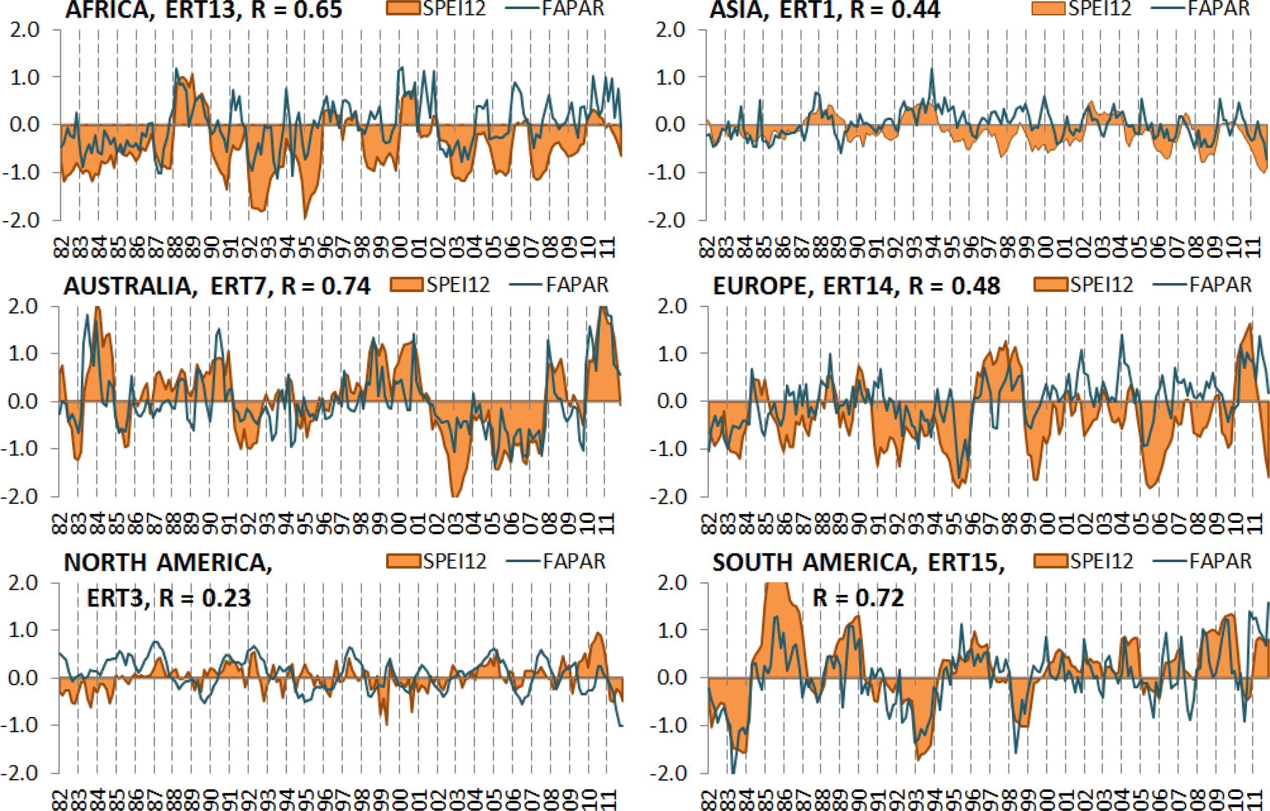
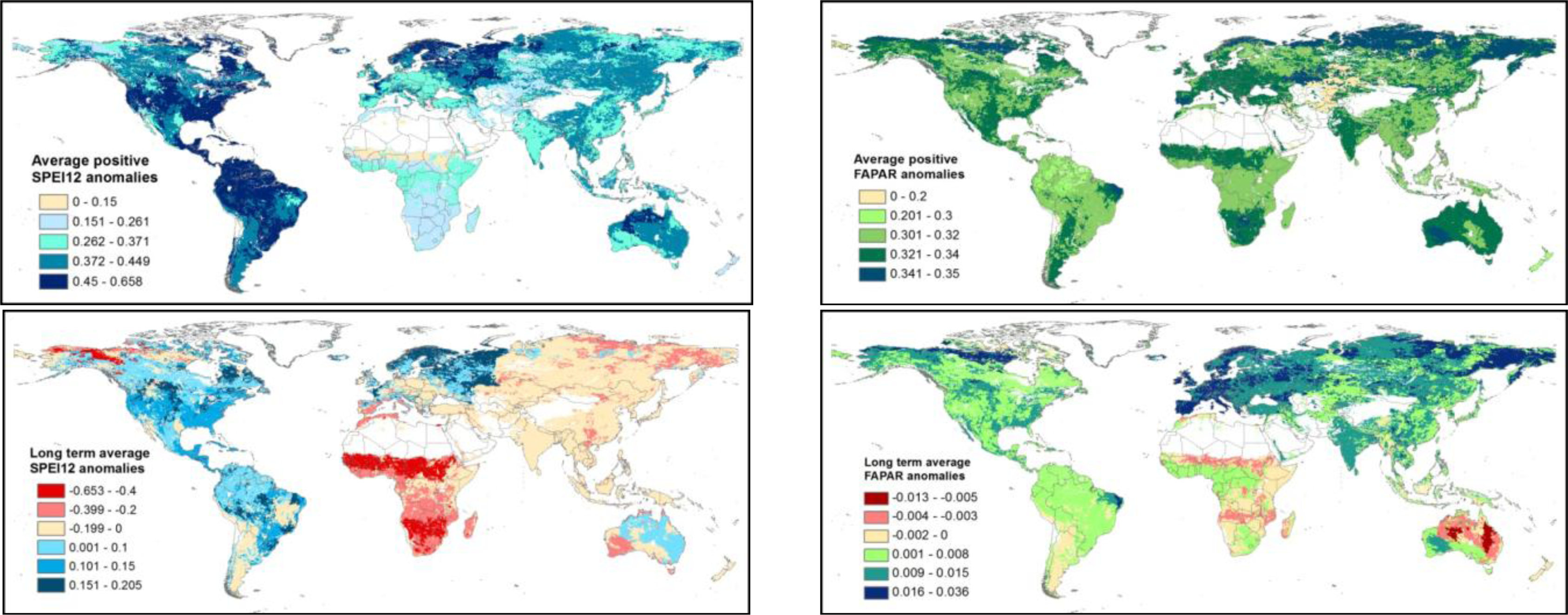
For both the SPEI12 (S) and the FPAR3g (F) time-series, we derived the average positive (SGT0 and FGT0), the average negative (SLT0 and FLT0), the long term average (SLTA and FLTA) and the long term non-parametric slope (Thiel-Sen statistics) values (TrdS and TrdF). Significance of the linear slope was not tested because the FPAR3g and SPEI12 anomaly series are mostly stochastic series following a unit root process (random walks) and thus these series cannot be modelled as a function of time. Although autoregressive models are able to parameterize stochastic trends in the present study, we were not interested in the significance of the trend but merely in the long term positive and negative dynamics. Therefore, only the slope values were analyzed to indicate changes. Furthermore, for each ERT the average SPIE12 time-profiles were derived (1982–2011) and these were correlated with the FPAR3g anomalies for each pixel within the given ERT (R).
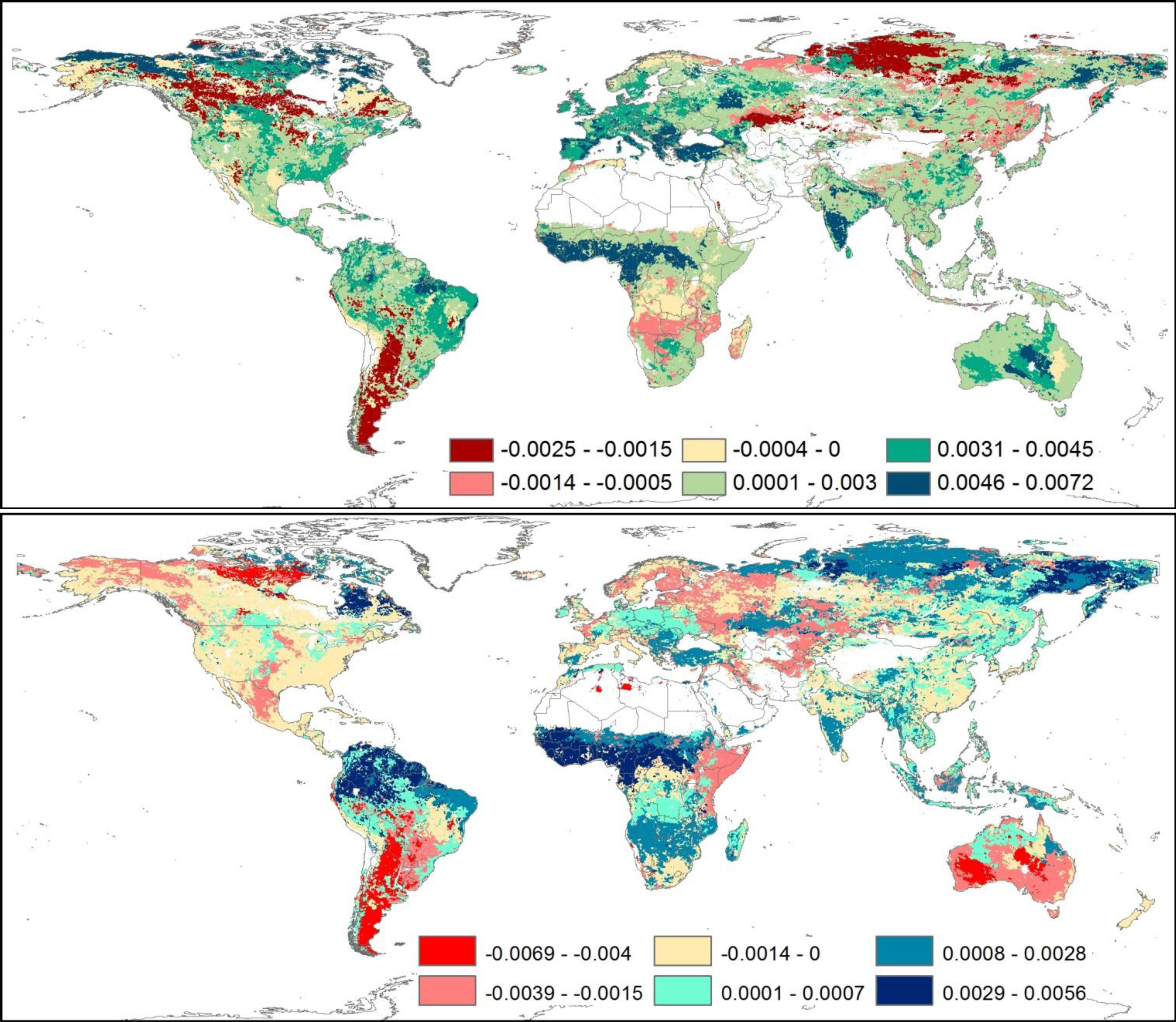
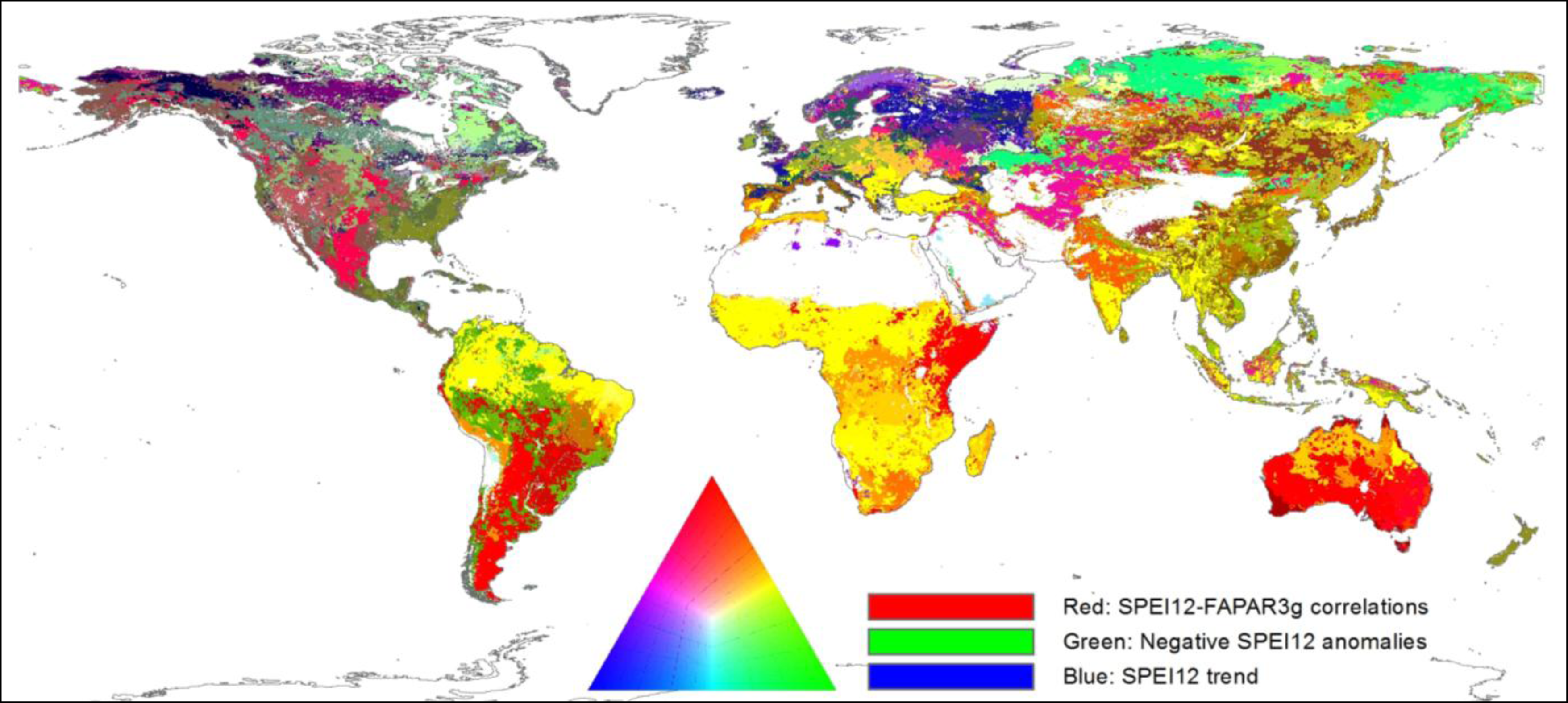
A red-green-blue color composite of R (red channel), TrdS (green channel) and SLT0 (blue channel) was prepared to identify global ERTs with similar climate-vegetation cover dynamics. The long term SPEI12 and FPAR3g temporal profiles for each ERT are provided in the Supplementary Materials section, which enhance the understanding of the timing, duration, frequency and severity of the climatic anomalies in the ERTs as well as correlating vegetation cover dynamics.
If the ERTs correctly describe drought and vegetation change types of ecosystems, their SPEI12 and FPAR3g anomalies and trends should be significantly different. To test this assumption, one-way univariate Anovas were run for each continent separately with the SPEI12 and FPAR3g variables as dependents and the ERTs as predictors. Model significance and the adjusted R2 measure were used to test the amount of variance in the SPEI12 and FPAR3g variables that the ERTs explained.
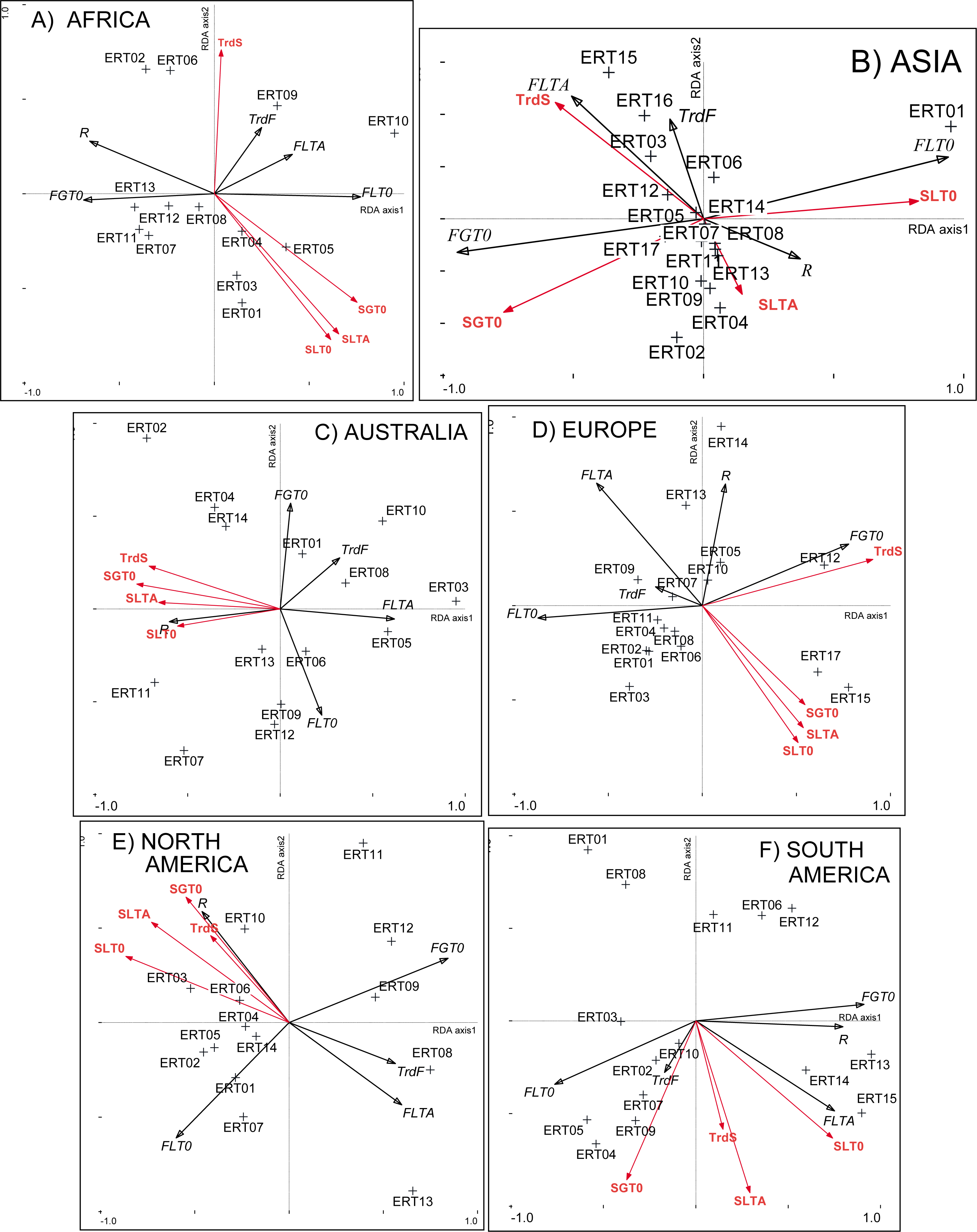
A gradient analysis was run using a Redundancy Analysis (RDA) as in [42] to assess how much of the variance in the FPAR3g dataset can be explained by the SPEI12 data. The input for this analysis was a data table for each continent separately with the ERTs as rows and FPAR3g and SPEI12 variables averaged within the ERTs as columns. Results were presented as tri-plots with the ERTs, the FPAR3g variables and the SPEI12 predictors. Based on the position of the ERTs and the FPAR3g variables the indicator value of the metrics for a given ERT can be inferred. Projecting the ERTs perpendicularly onto one of the arrows of the FPAR3g or SPEI12 variables shows the value of the variable in that ERT. The SPEI12 and FPAR3g variables were presented by arrows. Arrows pointing in the same direction in the tri-plot indicate positive correlation of the variables whereas arrows being nearly perpendicular indicate no correlation between the variables.
3.5. Combined Effects of the ERTs, Climate Zones and Land Management in Relation to FPAR and SPEI12 Correlations
To further help the characterization of the ERTs, for each continent, one-way univariate Anovas were run with the FPAR3g-SPEI12 correlation values (R) as the dependent variables and the ERTs, land management classes and Köppen climate zones as explanatory factors. Two-way Anovas were used to test the combined effects of (1) ERTs and climate zones and (2) ERTs and land management classes in discriminating group means of the correlation values. We tested the significance of the models and the adjusted R2 measure was used to test the amount of variance in the climate-vegetation anomaly correlations explained by the ERTs, climate zones and their combinations.
4. Results
4.1. Classification of Ecosystem Response Types
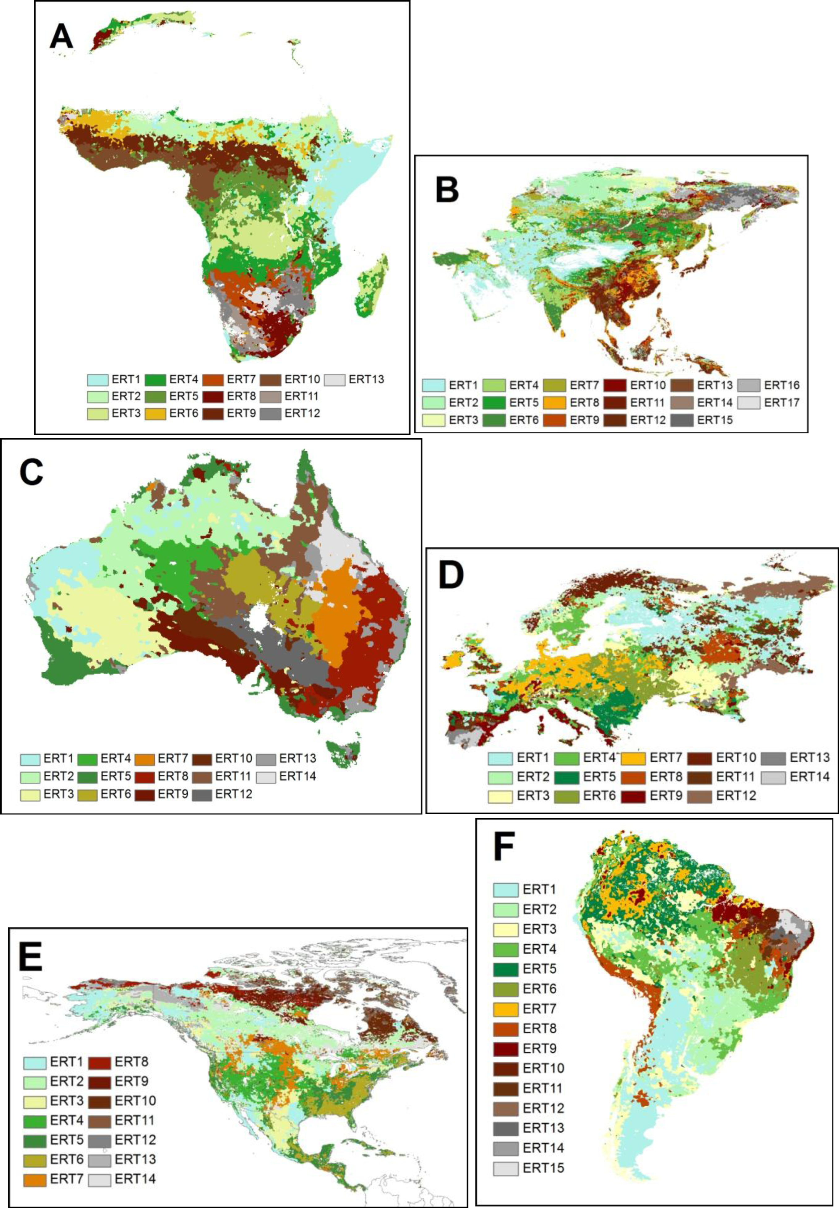
Figure 1 shows the classified Ecosystem Response Types (ERTs) per continent. All SPEI12 and FPAR3g correlations, anomalies and trends of the ERTs were significantly different (p < 0.001) for all continents indicating the unique information contents of all ERTs. Overall highest explanatory values of the ERTs were seen in Australia, Europe and South America (Table 1, adjusted R2) whereas least amount of variance in the SPEI12 and FPAR3g variables was explained by the ERTs in Asia. Globally, the variances in the SPEI12-FPAR3g correlations and in the FPAR3g trends were explained the best by the ERTs whereas weakest explanatory power was seen for long term average FPAR3g anomalies and for SPEI12 trends.
Figure 2 presents the red-green-blue color composite of the SPEI12-FPAR3g correlation (R, red channel), the trend in the SPEI12 anomalies (TrdS, green channel) and the strength of the negative SPEI12 anomalies (SLT0, blue channel). Red and orange toned ERTs represent areas with positive correlation between the SPEI12 and FPAR3g anomalies with anomalies being mostly negative and where trends in the SPEI12 are also negative. Thus, these areas were affected by several drought events between 1982 and 2011 with a strong negative effect on the vegetation, and the severity of the drought events also increased over these 30 years. These ERTs are found mostly in the Southern Hemisphere, notably over the southern part of Latin America (mostly over Argentina), the Horn of Africa and the southern part of Australia.
For ERTs shown in yellow and orange tones, the correlation between SPEI12 and FPAR3g anomalies is also due to droughts (positive correlation between mostly negative anomalies) but in these ERTs the severity of the drought events decreased over the last 30 years (positive SPEI12 trends). These ERTs are mostly found in Asia (India, China and Indochina Peninsula), the Mediterranean and south-east areas of Europe, most parts of Africa, northern Australia and northern parts of Latin America.
For ERTs depicted in bluish and purple tones, the negative SPEI12 anomalies were weak or positive and the correlation between the SPEI12 and the FPAR3g anomalies was negative. However, over these areas the SPEI12 expressed a negative trend in the anomalies, thus an increase in the severity of drought events. These ERTs are mostly found in the Northern Hemisphere over Canada, Alaska, Atlantic and northern Europe. ERTs shown in cyan tones (e.g., in Northern Asia) are indicating negative correlation between the SPEI12 and FPAR3g anomalies, moderate to strong negative SPEI12 anomalies but a positive trend in the SPEI12 anomalies. Thus, in these ERTs, negative SPEI12 anomalies did not affect vegetation development as also seen in the generally positive FPAR3g trends.
4.2. Long Term SPEI12 and FPAR3g Dynamics of the ERTs
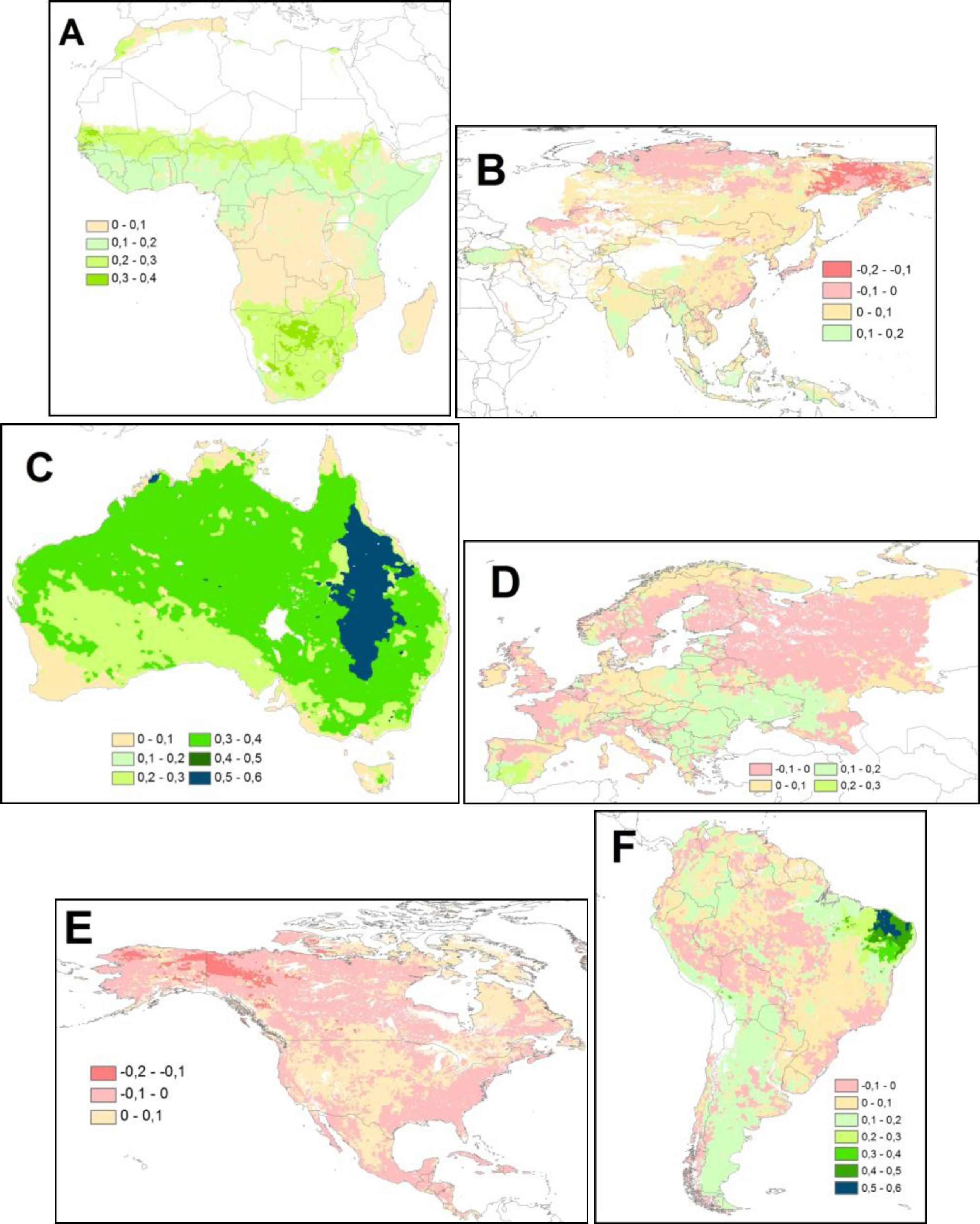
In Africa, strongest correlations (R) between SPEI12 and FPAR3g anomalies were observed in Mozambique (ERT12 and ERT13), over the Sahel (ERT2 and ECT6), and over northern and southern Namibia (ERT7 and ERT11, Figures 3A and 4A). In the Sahel, ERTs (ERT2 and ERT6) and in ERT13 (Mozambique) the SPEI12 anomalies (Figure 5) were negative and the average negative anomalies were very strong indicating that during the 30 years, several drought events affected these areas (see Figure 6 for an example over ERT13). Despite these drought events, trends (Figure 7) in SPEI12 and FPAR3g over the Sahel were positive whereas in ERTs 7 and 11 (Namibia) and in ERT12 (Mozambique) both SPEI12 and FPAR3g showed negative trends. Weakest correlation between the SPEI12 and FPAR3g anomalies was seen in the tropical and sub-tropical regions (ERT3, ERT4, and ERT5). Whereas ERT3 and ERT5 showed increasing vegetation cover, in the sub-tropical region of ERT4 decreasing productivity was observed. Despite positive long term average and moderate negative SPEI12 anomalies (Figure 5) the Horn of Africa (ERT1) showed one of the strongest negative SPEI12 trends (Figure 7) on the continent indicating increasing severity of droughts.
In Asia, strongest SPEI12-FPAR3g correlations were observed in ERT1 over Iraq, east of the Caspian Sea and south Russia, in ERT6 in India and Turkey and in ERT12 mostly over south China, Burma and Thailand (Figures 3B and 4B). In these ERTs, the long term average anomalies (Figure 5) were negative but the negative anomalies were not strong indicating that during the 30 years, drought did not affected these areas (See Figure 6 for an example in ERT1). In ERT1, both the SPEI12 and the FPAR3g anomalies expressed slight negative trends whereas in ERT6 and in ERT12 both SPEI12 and FPAR3g trends were positive (Figure 7). Weakest correlations were seen in the ERTs over the Siberian regions (ERT02 and ERT03) and north-east Russia over Siberia and the Cherskiy Range (ERTs 15 and 16). In ERT15 and ERT16, the SPEI12 anomalies were weak (Figure 5) but showed an increasing trend and also the vegetation vigor showed one of the strongest positive trends, whereas over the Siberian regions mostly decreasing FPAR3g trends were seen (Figure 7).
In Australia, the SPEI12-FPAR3g correlations of the ERTs were positive across the whole continent (Figures 3C and 4C). Strongest correlation was observed in ERT7 (Great Artesian Basin, Figure 3), ERT11 (north-west of the Great Artesian Basin), ERT14 (Queensland), ERT12 in the south central part, and in ERT1 (Hamersley Range and North West Basin). Only ERT5 over the south-west and north shores (Arnhem Land and the Cape York Peninsula), ERT9 over the south shores along the Great Australian Bight and ERT3 over the north-western part of the continent showed weaker correlations. In these ERTs, the long term average SPIE12 anomalies were negative and the negative SPEI12 anomalies were strong (Figure 5) with a strong negative trend but the FPAR3g did not express pronounced trends (Figure 7). ERT7 (Great Artesian Basin) and ERT1 (Hamersley Range and North West Basin) showed the strongest negative trend in the FPAR3g (Figure 7) and the correlation to the SPEI12 anomalies were very strong thus here the productivity loss can be attributed to climatic fluctuations.
In Europe, ERTs 14 and 13 in the southern part of the Iberian peninsula and ERT5 over south-eastern Europe showed the strongest correlation between SPEI12 and FPAR3g and moderate correlations were seen in ERT9 covering the coastal Mediterranean areas (Figures 3D and 4D). In these ECTs, the long term average SPEI12 anomalies were negative and the negative anomalies were very strong (Figure 5) indicating that several drought events affected these areas over the 30 years (see Figure 6 for ERT14). However, despite the drought events, positive trends were observed in the SPEI12 correlating with positive FPAR3g trends (Figure 7). In fact, ERT9 exhibited the strongest positive FPAR3g trend on the continent. Weakest correlations were seen in the ERTs over northern and Atlantic Europe (ERT01 and ERT03) and in forests and sparsely vegetated areas of ERT4 and in forests and wetlands of ERT11. In these areas, droughts did not severely affect vegetation development in the 30-year period as a positive trend was observed in the FPAR3g (Figure 7).
In North America, ERT3 (mostly the Sierra Madre) and ERT4 (north of the Sierra Madre) showed the strongest correlation between SPEI12 and FPAR3g (Figures 3E and 4E) but these correlations were the weakest in global comparison. In these ERTs, the long term average SPEI12 anomalies were positive (Figure 5) indicating that these areas were not subject to pronounced effects of droughts but the SPEI12 trends were negative point to drying conditions. The vegetation dynamics fluctuated with weak positive and negative anomalies and moderately positive FPAR3g trends (Figure 7). Weakest correlations were seen in the ERT13 (north-west Canada bordering Alaska) with strong negative trends in the SPEI12 but strong positive trends in the FPAR3g (Figure 7). Also, ERT14, distributed over the continent, showed strong negative correlation between SPEI12 and FPAR3g anomalies but here the SPEI12 trends were negative and the positive trend in vegetation cover was moderate (Figure 7).
In South America, strongest positive correlation between SPEI12 and FPAR3g was observed in ERTs 12, 13, 14 and 15 over the western coastal areas in Brazil (Figures 3F and 4F). In these ERTs the SPEI12 anomalies expressed weak negative and positive fluctuations and positive trends and the anomalies and trend in the vegetation cover were generally positive as well (Figures 5 and 7). In ERT1 (Argentinean Pampas) on the other hand, the strong correlation between SPEI12 and FPAR3g was accompanied by negative long term average and very strong negative anomalies together with a decreasing trend in the SPEI12. Thus, the strong decrease in the vegetation activity in these areas is likely to be attributed to drought events. Strongest negative correlation between the SPEI12 and FPAR3g anomalies was observed over the tropical areas (ERT3 and ERT4) where neither the FPAR3g nor the SPEI12 expressed strong trends or fluctuations.
4.3. Combined Effects of the ERTs, Climate Zones and Land Management in Explaining FPAR3g and SPEI12 Correlations
In Africa, the variance in SPEI12-FPAR3g correlation explained by the ERTs, Köppen zones and land management classes was generally moderate. Most variance was explained by the ERTs (adjusted R2 of 0.388, Table 2), the effect of climate zones was lower (adjusted R2 of 0.134) and that of management was very low (adjusted R2 of 0.070). Highest explanatory value was seen when the ECTs were analyzed together with their respective management classes (adjusted R2 of 0.460), which was only marginally higher than the explanatory value of ECTs and climate zones (adjusted R2 of 0.457).
In Asia, all Anova models explained a very low amount of variance in the SPEI12-FPAR3g correlation. Most variance was explained by the ERTs (adjusted R2 of 0.153) whereas the effect of climate zones and management classes were very low (adjusted R2 of 0.078 and 0.056, respectively). Highest explanatory value was seen when the ERTs were analyzed together with the climate zones (adjusted R2 of 0.209), which was only marginally higher than the explanatory value of the ERTs and their respective management classes (adjusted R2 of 0.192).
In Australia, most variance was explained by the ERTs (adjusted R2 = 0.541), the climate zones explained less variance (adjusted R2 = 0.319) whereas the effect of management classes was low (adjusted R2 = 0.128). Highest explanatory value was observed when the ERTs were analyzed together with the climate zones (adjusted R2 of 0.624), which was considerably higher than the explanatory value of ERTs and their respective management levels (adjusted R2 of 0.572).
In Europe, most variance in SPEI12-FPAR3g correlation was explained by the ERTs (adjusted R2 = 0.403), the climate zones explained much less variance (adjusted R2 = 0.147) whereas the effect of management classes were moderately higher (adjusted R2 = 0.171. Analyzing the ERTs together with the climate zones or with the land management classes increased the explanatory power of the single model with the ERTs only, but the two extra predictors of climate and land management had the same importance (adjusted R2 of 0.507 and 0.503, respectively).
In North America, the Anova models explained the very low amount of variance. North America was the only continent where the climate zones explained more variance than the ERTs (adjusted R2 = 0.159 vs. adjusted R2 = 0.146) whereas the effect of land management was very low (adjusted R2 = 0.082). Highest explanatory value was seen when the ERTs were analyzed together with the climate zones (adjusted R2 of 0.318), which was considerably higher than the explanatory value of ERTs and their respective management levels (adjusted R2 of 0.245).
The two-way Anova models of South America explained the highest amount of variance in the SPEI12-FPAR3g correlations of all continents. Most variance was explained by the ERTs (adjusted R2 = 0.553), the climate zones explained much less variance (adjusted R2 = 0.181) whereas the effect of management classes was moderate (adjusted R2 = 0.106). Highest explanatory value was seen when the ERTs were analyzed together with the climate zones (adjusted R2 of 0.654), which was moderately higher than the explanatory value of ERTs and their respective management levels (adjusted R2 of 0.609).
5. Discussion
5.1. Ecosystems with Positive SPEI12-FPAR3g Correlations
Ecosystem Response Types (ERTs) presenting the strongest correlation between SPEI12 and FPAR3g anomalies were mainly found in semi-arid areas and in areas where water is a major climate constrain [43], e.g., in Australia (Great Artesian Basin, Queensland, south-central part, Hamersley Range and North West Basin and north-west of the Great Artesian Basin), South America (North-Eastern Brazil and Argentina) and in Africa (part of the Sahel and Southern Africa). However, a positive correlation between SPEI12 and FPAR3g does not necessarily indicate increasing severity of drought as despite intense droughts and heat waves [44], some of these regions were also reported as areas of increased vegetation activity due to relaxation of climatic constraints to plant growth [24,26,28,45].
In the Sahel region, for instance, the most severe droughts occurred in the 80s but greening trends were observed in the last decades. Our study showed that these greening trends are associated with positive trends in the SPEI12 in line with [46] showing increases in daily rainfall intensity over these areas. The same authors projected an overall wetter Sahel with more variable precipitation on all time scales; thus, in the future, if these trends follow the observed pattern, these areas might be less at risk of losing productivity due to droughts. North-east of Brazil showed globally one of the strongest correlations between FPAR3g and SPEI12 and also here trends in both SPEI12 and FPAR3g anomalies were positive. In 2013, however, after the observation period of this study, north-eastern Brazil suffered its worst drought in the last 50 years.
In Argentina, the positive FPAR3g-SPEI12 correlations were coupled with negative long term average and very strong negative SPEI12 anomalies together with strongly matching spatial patterns of negative SPEI12 and negative FPAR3g trends. Although [47] attributed the decreased productivity in Argentina to agricultural expansion, our results suggest that droughts may also have contributed to productivity decline. In Australia, the correlation between vegetation responses to SPEI12 anomalies was very strong for most of the continent but trends in FPAR3g were mostly positive (probably due to the extreme wet years in 2010 and 2011, Bureau of Meteorology. Nevertheless, also here drought has returned by 2013; in western Queensland, rainfall has been 48% below average. This indicates the necessity of regular monitoring of ecosystems’ response to drought and extreme climate events but also the need for methodological research for assessing the gradual and abrupt changes in ecosystem responses [48].
5.2. Ecosystems with Negative SPEI12-FPAR3g Correlation and Increasing Vegetation Activity
Weak or negative SPEI12-FPAR3g correlation but positive trends in FPAR3g anomalies were observed in North America (Boreal forest region of Canada and Alaska), Asia (Siberia and the Cherskiy Range) and Europe (continental areas, the Don-Plain west of the Volga, Northern Scandinavia), areas where precipitation is no longer the primary constraint of vegetation growth and therefore a strong correlation cannot be expected. The positive trends in vegetation activity are in line with [40] reporting greening in the Northern Hemisphere but the same authors showed correlation to increasing temperature and precipitation which is not confirmed by the present study. A decade later [49] reported that trends have stalled or even inversed. These results indicate again the necessity or regular monitoring of changes in anomalies and trends but might also indicate that (1) the same climatic indicator might not be equally useful in different ecosystems; (2) drought indicators may not be appropriate in Northern, mostly temperature limited ecosystems; or (3) terrestrial biomes response to different SPEI time-scales [50].
5.3. Ecosystems with Negative SPEI12-FPAR3g Correlation and Decreasing Vegetation Activity
Negative SPEI12-FPAR3g correlation together with decreased vegetation productivity was mostly observed in North America, North-West Russia, Asia and in the tropical ecosystems. In North-West Russia, the negative SPEI12 anomalies were moderate with increasing SPEI12 trends thus the decrease in vegetation activity should be associated to other factors than climatic fluctuations. In North America, mostly the Boreal forest of Canada exhibited decreased vegetation productivity. Here, the SPEI12 trend map reveals a negative SPEI12 trend and thus this area seems to be affected by a decrease in precipitation and thus an increase in vapour pressure deficit. These results are in line with [48] where long periods of browning were observed in boreal forest of Canada and Siberia, in which drought and vapour pressure deficit were reported as possible drivers [51]. Other authors also reported productivity decline of North American forests attributed to late summer droughts [52,53]. In Asia, the Siberian forests and the widespread ERT7 with natural vegetation showed no reaction to drought fluctuations but strong negative FPAR3g trends. Contrary to the North American Boreal regions, here increased trends were seen in the SPEI12 anomalies whereas the strength of the anomalies remained weak. Therefore, here the loss in vegetation productivity cannot be attributed to extreme weather conditions and, as such, the origin lies most probably in other influencing factors such as, e.g., intensive human use.
Negative correlation of the FPAR3g to the SPEI12 in the Amazon contributes to the scientific discussion on controversial results. The International Panel on Climate Change [5] reported 40% of the Amazon region is highly vulnerable to drought but [54] found greening up in the Amazon after the 2005 drought. These results were found irreproducible when looking at the same data by [55]. Using ground data, the study of [56] showed that after the 2005 drought affected forest lost biomass and impacts were greatest where the dry season was intense. Our results are similar to e.g. [55] showing no correlation between drought severity and greenness changes in the Amazon region, but we raise caution, similarly to [57], that uncertainties around different scientific results might also arise due to the limit of the spatial resolution or sensor characteristics of remote sensing data in assessing local effects of droughts.
5.4. ERTs, Climate Zones and Land Management Differences of SPEI12-FPAR3g Correlations
The implemented ISODATA algorithm herein leaves space for improvement because depending on the analysis domain, the resulting clusters will change. As the various spatial scales will result in different cluster sizes, the ERTs can be only considered valid representations of ecosystems’ responses to SPEI12 fluctuation on the here presented continental scale. Our attempts to attribute correlations of SPEI12 and FPAR3g to land management did not significantly improve understanding of the observed spatio-temporal patterns of co-varying drought and vegetation anomalies. Only in Europe had land management higher explanatory value in SPEI12-FPAR3g correlation than climate zones. This indicates that in very intensively managed European ecosystems, land use and management intensity strongly influence the impacts of drought on the ecosystem. These outcomes are important for food security studies and further research should look more into the effect of land use in resilience to drought. On the other hand, the generally low explanatory value of land management classes in areas other than Europe might also indicate the necessity to improve information on land use and its intensity.
When the ERTs were analyzed together with the climate zones, the explanatory power of the Anova models increased and was higher than the combined effect of the ERTs and land management. Only in Africa did the combination of land use and ERTs explain slightly more variation in drought-vegetation correlation than the combination of ERTs and climate. This might indicate the need to update recent climate zoning of ecosystems introducing higher thematic details. On the other hand, the reason for the similar explanatory value of climate zones and land use might also lie in their complex and interactive patterns [58,59]. Furthermore, large interregional differences were reported especially in the Sahel in the greening and browning trends [60], indicating small scale heterogeneity in vegetation dynamics that current climate classification might have difficulties in tackling. This is in line with another study [61] indicating that, in the Sahel, vegetation is more influenced by natural processes than by humans.
The lowest amount of variance in the correlation of SPEI12 and FPAR3g anomalies was explained in North America and Asia regarding both the ERTs and the land use classes. North America was the only continent were the climate zones accounted for more variance than the ERTs, and although this was low, the explained variance has increased considerably when accounting for their combined effect. This is consistent with other results in this study indicating mostly weak correlations between the FPAR3g and SPEI12 in North America. In Asia, on the other hand, the explanatory power of the ERTs has not improved considerably when accounting for the effects of climate zones or land management. This indicates that in Asia the climate-vegetation anomaly correlation developed in a more complex way in the last 30 years than in other continents, and for the correct characterization, other factors such as land use change should most probably be also considered.
6. Concluding Remarks
Understanding the interactions between climate, vegetation and human systems is a key issue for researchers studying climate impacts on the terrestrial ecosystems as well as for managers in charge of land uses allocations. While observing trends in global vegetation developments are undoubtedly important in global change studies, attributing these trends to climate variations in a spatially explicit way represents a further step in understanding global Earth system changes. In this study, we showed that the typology of responses in global ecosystems can be identified by analyzing the spatio-temporal co-variability between time-series of SPEI12 and FPAR3g anomalies. Mapping Ecosystem Response Types (ERTs) with the here presented methodology enabled the combined assessment of the location, timing, duration, frequency and severity of climatic anomalies with the joint assessment of wetting and drying climatic conditions. Although the analysis domain affects classification results, we showed that these Ecosystems Change Types correspond to region specific spatio-temporal patterns of co-variation between SPEI12 and FPAR3g anomalies reflecting ecosystem response to fluctuations in climatic anomalies. Although attributing correlations of SPEI12 and FPAR3g to land management did not significantly improve understanding of the observed spatio-temporal patterns of climate-vegetation cover anomalies, the methodology has the potential to further support global change studies.
Acknowledgments
The authors thank C.J. Tucker and J. Pinzon of NASA GSFC and Ranga Myneni (Department of Earth & Environment, Boston University) for producing and sharing the AVHRR GIMMS3g NDVI and FPAR3g dataset. The authors wish to express their gratitude to Josh Hooker, currently working at the EC Joint Research Centre, for helping with the matrix algebra of the combined PCA analysis. This research was partly funded by the Danish Council for Independent Research (DFF) Sapere Aude programme; project entitled “Earth Observation based Vegetation productivity and Land Degradation Trends in Global Drylands”.
Author Contributions
Eva Ivits developed the methodology, performed the analysis and wrote the main body of the text. Stephanie Horion, Rasmus Fensholt and Michael Cherlet participated in formulating the research question, placing the analysis in the global context and formulating the discussion. All authors read and improved the manuscript and discussed the results
Conflicts of Interest
The authors declare no conflict of interest.
References
- M, L.; Canziani, O.F.; Palutikof, J.P.; van der Linden, P.J.; Hanson, C.E. Climate Change 2007: Impacts, Adaptation and Vulnerability; Cambridge University Press: Cambridge, UK, 2007. [Google Scholar]
- Woodward, F.I.; Lomas, M.R.; Kelly, C.K. Global climate and the distribution of plant biomes. Philos. Trans. Roy. Soc. B: Biol. Sci 2004, 359, 1465–1476. [Google Scholar]
- Millennium Ecosystem Assessment. In Ecosystems and Human Well-being: Synthesis; Island Press: Washington, DC, USA, 2005.
- Huntington, T.G. Evidence for intensification of the global water cycle: Review and synthesis. J. Hydrol 2006, 319, 83–95. [Google Scholar]
- Solomon, S.D.; Manning, Q.M.; Chen, Z.; Marquis, M.; Avery, K.B.; Tignor, M.; Miller, H.L. Climate Change 2007: The Physical Science Basis; Cambridge University Press: Cambridge, UK, 2007. [Google Scholar]
- Tebaldi, C.; Hayhoe, K.; Arblaster, J.; Meehl, G. Going to the extremes: An intercomparison of model-simulated historical and future changes in extreme events. Clim. Chang 2006, 79, 185–211. [Google Scholar]
- Rockström, J.; Steffen, W.; Noone, K.; Persson, Å.; Chapin, F.S., III; Lambin, E.F.; Lenton, T.M.; Scheffer, M.; Folke, C.; Schellnhuber, H.J.; et al. A safe operating space for humanity. Nature 2009, 461, 472–475. [Google Scholar]
- Holling, C.S. Understanding the complexity of economic, ecological, and social systems. Ecosystems 2001, 4, 390–405. [Google Scholar]
- Lenton, T.M.; Held, H.; Kriegler, E.; Hall, J.W.; Lucht, W.; Rahmstorf, S.; Schellnhuber, H.J. Tipping elements in the Earth’s climate system. Proc. Natl. Acad. Sci 2008, 105, 1786–1793. [Google Scholar]
- Rustad, L.E. The response of terrestrial ecosystems to global climate change: Towards an integrated approach. Sci. Total Environ 2008, 404, 222–235. [Google Scholar]
- Loreau, M.; Naeem, S.; Inchausti, P. Biodiversity and Ecosystem Functioning: Synthesis and Perspectives; Oxford University Press Inc: New York, NY, USA, 2002. [Google Scholar]
- Hooper, D.U.; Chapin, F.S., III; Ewel, J.J.; HECTor, A.; Inchausti, P.; Lavorel, S.; Lawton, J.H.; Lodge, D.M.; Loreau, M.; Naeem, S.; et al. Effects of biodiversity on ecosystem functioning: A consensus of current knowledge. Ecol. Monogr 2005, 75, 3–35. [Google Scholar]
- Tilman, D. Ecological consequences of biodiversity: A search for general principles. Ecology 1999, 80, 1455–1474. [Google Scholar]
- Wardle, D.A.; Bardgett, R.D.; Callaway, R.M.; van der Putten, W.H. Terrestrial ecosystem responses to species gains and losses. Science 2011, 332, 1273–1277. [Google Scholar]
- Balvanera, P.; Pfisterer, A.B.; Buchmann, N.; He, J.S.; Nakashizuka, T.; Raffaelli, D.; Schmid, B. Quantifying the evidence for biodiversity effects on ecosystem functioning and services. Ecol. Lett 2006, 9, 1146–1156. [Google Scholar]
- Cardinale, B.J.; Matulich, K.L.; Hooper, D.U.; Byrnes, J.E.; Duffy, E.; Gamfeldt, L.; Balvanera, P.; O’Connor, M.I.; Gonzalez, A. The functional role of producer diversity in ecosystems. Am. J. Bot 2011, 98, 572–592. [Google Scholar]
- Tallis, H.; Mooney, H.; Andelman, S.; Balvanera, P.; Cramer, W.; Karp, D.; Polasky, S.; Reyers, B.; Ricketts, T.; Running, S.; et al. A global system for monitoring ecosystem service change. BioScience 2012, 62, 977–986. [Google Scholar]
- Van Leeuwen, W.J.; Hartfield, K.; Miranda, M.; Meza, F.J. Trends and ENSO/AAO driven variability in NDVI derived productivity and phenology alongside the Andes Mountains. Remote Sens 2013, 5, 1177–1203. [Google Scholar]
- Jiang, N.; Zhu, W.; Zheng, Z.; Chen, G.; Fan, D. A comparative analysis between GIMSS NDVIg and NDVI3g for monitoring vegetation activity change in the Northern Hemisphere during 1982–2008. Remote Sens 2013, 5, 4031–4044. [Google Scholar]
- Vrieling, A.; de Leeuw, J.; Said, M.Y. Length of growing period over Africa: Variability and trends from 30 years of NDVI time series. Remote Sens 2013, 5, 982–1000. [Google Scholar]
- Ivits, E.; Cherlet, M.; Tóth, G.; Sommer, S.; Mehl, W.; Vogt, J.; Micale, F. Combining satellite derived phenology with climate data for climate change impact assessment. Glob. Planet. Chang 2012. [Google Scholar] [CrossRef]
- Anyamba, A.; Tucker, C.J. Analysis of Sahelian vegetation dynamics using NOAA-AVHRR NDVI data from 1981–2003. J. Arid Environ 2005, 63, 596–614. [Google Scholar]
- Forkel, M.; Carvalhais, N.; Verbesselt, J.; Mahecha, M.D.; Neigh, C.S.; Reichstein, M. Trend change detectionin NDVI time series: Effects of inter-annual variability and methodology. Remote Sens 2013, 5, 2113–2144. [Google Scholar]
- Mao, J.; Shi, X.; Thornton, P.E.; Hoffman, F.M.; Zhu, Z.; Myneni, R.B. Global latitudinal-asymmetric vegetation growth trends and their driving mechanisms: 1982–2009. Remote Sens 2013, 5, 1484–1497. [Google Scholar]
- Zhao, X.; Liang, S.; Liu, S.; Yuan, W.; Xiao, Z.; Liu, Q.; Cheng, J.; Zhang, X.; Tang, H.; Zhang, X.; et al. The Global Land Surface Satellite (GLASS) remote sensing data processing system and products. Remote Sens 2013, 5, 2436–2450. [Google Scholar]
- Nemani, R.R.; Keeling, C.D.; Hashimoto, H.; Jolly, W.M.; Piper, S.C.; Tucker, C.J.; Myneni, R.B.; Running, S.W. Climate-driven increases in global terrestrial net primary production from 1982 to 1999. Science 2003, 300, 1560–1563. [Google Scholar]
- Campo-Bescós, M.A.; Muñoz-Carpena, R.; Southworth, J.; Zhu, L.; Waylen, P.R.; Bunting, E. Combined spatizal and temporal effects of environmental controls on long-term monthly NDVI in the Southern Africa Savanna. Remote Sens 2013, 5, 6513–6538. [Google Scholar]
- Fensholt, R.; Langanke, T.; Rasmussen, K.; Reenberg, A.; Prince, S.D.; Tucker, C.; Scholes, R.J.; Le, Q.B.; Bondeau, A.; Eastman, R.; et al. Greenness in semi-arid areas across the globe 1981–2007—An earth observing satellite based analysis of trends and drivers. Remote Sens. Environ 2012, 121, 144–158. [Google Scholar]
- Fensholt, R.; Rasmussen, K. Analysis of trends in the Sahelian “rain-use efficiency” using GIMMS NDVI, RFE and GPCP rainfall data. Remote Sens. Environ 2011, 115, 438–451. [Google Scholar]
- Kariyeva, J.; van Leeuwen, W.J.D. Environmental drivers of NDVI-based vegetation phenology in Central Asia. Remote Sens 2011, 3, 203–246. [Google Scholar]
- Van Leeuwen, W.J.D. Monitoring the effects of forest restoration treatments on post-fire vegetation recovery with MODIS multitemporal data. Sensors 2008, 8, 2017–2042. [Google Scholar]
- Herrmann, S.M.; Anyamba, A.; Tucker, C.J. Recent trends in vegetation dynamics in the African Sahel and their relationship to climate. Glob. Environ. Chang 2005, 15, 394–404. [Google Scholar]
- Knapp, A.K.; Smith, M.D. Variation among biomes in temporal dynamics of aboveground primary production. Science 2001, 291, 481–484. [Google Scholar]
- Vicente-Serrano, S.M.; Beguería, S.; López-Moreno, J.I. A multi-scalar drought index sensitive to global warming: The standardized precipitation evapotranspiration index. J. Clim 2010, 23, 1696–1718. [Google Scholar]
- Bordi, I.; Sutera, A. Fifty years of precipitation: Some spatially remote teleconnections. Water Resour. Manag 2001, 15, 247–280. [Google Scholar]
- Zhu, Z.; Bi, J.; Pan, Y.; Ganguly, S.; Anav, A.; Xu, L.; Samanta, A.; Piao, S.; Nemani, R.R.; Myneni, R.B. Global data sets of vegetation Leaf Area Index (LAI)3g and Fraction of Photosynthetically Active Radiation (FPAR)3g derived from Global Inventory Modeling and Mapping Studies (GIMMS) Normalized Difference Vegetation Index (NDVI3g) for the period 1981 to 2011. Remote Sens 2013, 5, 927–948. [Google Scholar]
- Pinzon, J.E.; Tucker, C.J. Revisiting error, precision and uncertainty in NDVI AVHRR data: Development of a consistent NDVI3g time series. Remote Sens 2014. under review.. [Google Scholar]
- Kottek, M.; Grieser, J.; Beck, C.; Rudolf, B.; Rubel, F. World map of the Köppen-Geiger climate classification updated. Meteorol. Z 2006, 15, 259–263. [Google Scholar]
- Nachtergaele, F.; Petri, M. Land Degradation Assessment in Drylands: Mapping Land Use Systems at Global and Regional Scales for Land Degradation Assessment Analysis; Food Agriculture Organization United Nation: Rome, Italy, 2011. [Google Scholar]
- Zhou, L.; Tucker, C.J.; Kaufmann, R.K.; Slayback, D.A.; Shabanov, N.V.; Myneni, R.B. Variations in northern vegetation activity inferred from satellite data of vegetation index during 1981 to 1999. J. Geophys. Res 2001, 106, 20269–20283. [Google Scholar]
- Wulder, M.; Boots, B. Local spatial autocorrelation characteristics of remotely sensed imagery assessed with the Getis statistic. Int. J. Remote Sens 1998, 19, 2223–2231. [Google Scholar]
- Ivits, E.; Cherlet, M.; Horion, S.; Fensholt, R. Global biogeographical pattern of ecosystem functional types derived from earth observation data. Remote Sens 2013, 5, 3305–3330. [Google Scholar]
- Churkina, G.; Running, S.W. Contrasting climatic controls on the estimated productivity of global terrestrial biomes. Ecosystems 1998, 1, 206–215. [Google Scholar]
- Heffernan, O. The dry facts. Nature 2013, 501, S2–S3. [Google Scholar]
- Zhao, M.; Running, S.W. Drought-induced reduction in global terrestrial net primary production from 2000 through 2009. Science 2010, 329, 940–943. [Google Scholar]
- Giannini, A.; Salack, S.; Lodoun, T.; Ali, A.; Gaye, A.T.; Ndiaye, O. A unifying view of climate change in the Sahel linking intra-seasonal, interannual and longer time scales. Environ. Res. Lett 2013, 8, 1–8. [Google Scholar]
- Viglizzo, E.F.; Frank, F.C.; Carreno, L.V.; Jobbágy, E.G.; Pereyra, H.; Clatt, J.; Pincén, D.; Ricard, M.F. Ecological and environmental footprint of 50 years of agricultural expansion in Argentina. Glob. Chang. Biol 2011, 17, 959–973. [Google Scholar]
- DeJong, R.; Verbesselt, J.; Schaepman, M.E.; de Bruin, S. Trend changes in global greening and browning: Contribution of short-term trends to longer-term change. Glob. Chang. Biol 2012, 18, 642–655. [Google Scholar]
- Wang, X.; Piao, S.; Ciais, P.; Li, J.; Friedlingstein, P.; Koven, C.; Chen, A. Spring temperature change and its implication in the change of vegetation growth in North America from 1982 to 2006. Proc. Natl. Acad. Sci 2011, 108, 1240–1245. [Google Scholar]
- Vicente-Serrano, S.M.; Gouveia, C.; Camarerod, J.J.; Begueríae, S.; Trigo, R.; López-Moreno, J.I.; Azorín-Molina, C.; Pasho, E.; Lorenzo-Lacruz, J.; Revuelto, J.; et al. Response of vegetation to drought time-scales across global land biomes. Proc. Natl. Acad. Sci 2013, 110, 52–57. [Google Scholar]
- Bunn, A.G.; Goetz, S.J.; Kimball, J.S.; Zhang, K. Northern high-latitude ecosystems respond to climate change. Eos Trans. American Geophys.Union 2007, 88, 333–340. [Google Scholar]
- Zhang, K.; Kimball, J.S.; Mu, Q.; Jones, L.A.; Goetz, S.J.; Running, S.W. Satellite based analysis of northern ET trends and associated changes in the regional water balance from 1983 to 2005. J. Hydrol 2009, 379, 92–110. [Google Scholar]
- Goetz, S.J.; Epstein, H.E.; Bhatt, U.S.; Jia, G.J.; Kaplan, J.O.; Lischke, H.; Yu, Q.; Bunn, A.; Lloyd, A.H.; Alcaraz-Segura, D.; et al. Recent Changes in Arctic Vegetation: Satellite Observations and Simulation Model Predictions. In Eurasian Arctic Land Cover and Land Use in a Changing Climate; Gutman, G., Reissell, A., Eds.; Springer: Amsterdam, The Netherlands, 2011; pp. 9–36. [Google Scholar]
- Saleska, S.R.; Didan, K.; Huete, A.R.; da Rocha, H.R. Amazon Forests green-up during 2005 drought. Science 2005, 318. [Google Scholar] [CrossRef]
- Samanta, A.; Ganguly, S.; Hashimoto, H.; Devadiga, S.; Vermote, E.; Knyazikhin, Y.; Nemani, R.R.; Myneni, R.B. Amazon forests did not green-up during the 2005 drought. Geophys. Res. Lett 2010, 37. [Google Scholar] [CrossRef]
- Phillips, O.L.; Aragão, L.E.O.C.; Lewis, S.L.; Fisher, J.B.; Lloyd, J.; López-González, G.; Malhi, Y.; Monteagudo, A.; Peacock, J.; Quesada, C.A.; et al. Drought sensitivity of the Amazon Rainforest. Science 2009, 323, 1344–1347. [Google Scholar]
- Asner, G.P.; Alencar, A. drought impacts on the Amazon forest: The remote sensing perspective. New Phytol 2010, 187, 569–578. [Google Scholar]
- Bégué, A.; Vintrou, E; Ruelland, D; Claden, M; Dessay, N. Can a 25-year trend in Soudano-Sahelian vegetation dynamics be interpreted in terms of land use change? A remote sensing approach. Glob. Environ. Chang 2011, 21, 413–420. [Google Scholar]
- Hein, L.; De Ridder, N.; Hiernaux, P.; Leemans, R.; de Wit, A.; Schaepman, M.E. Desertification in the Sahel: Towards better accounting for ecosystem dynamics in the interpretation of remote sensing images. J. Arid Environ 2011, 75, 1164–1172. [Google Scholar]
- De Jong, R.; Schaepman, M.E.; Furrer, R.; de Bruin, S.; Verburg, P.H. Spatial relationship between climatologies and changes in global vegetation activity. Glob. Chang. Biol 2013, 19, 1953–1964. [Google Scholar]
- Fensholt, R.; Rasmussen, K.; Kaspersen, P.; Huber, S.; Horion, S.; Swinnen, E. Assessing land degradation/recovery in the African Sahel from long-term earth observation based primary productivity and precipitation relationships. Remote Sens 2013, 5, 664–686. [Google Scholar]


| FPAR3g/SPEI12 Data | Africa | Asia | Australia | Europe | North America | South America |
|---|---|---|---|---|---|---|
| R | 0.388 | 0.153 | 0.541 | 0.403 | 0.146 | 0.553 |
| FGT0 | 0.168 | 0.394 | 0.327 | 0.449 | 0.396 | 0.309 |
| FLT0 | 0.154 | 0.384 | 0.373 | 0.415 | 0.387 | 0.246 |
| FLTA | 0.054 | <0.001 | 0.229 | 0.096 | 0.054 | 0.087 |
| SGT0 | 0.235 | 0.186 | 0.297 | 0.053 | 0.353 | 0.164 |
| SLT0 | 0.337 | 0.184 | 0.317 | 0.435 | 0.102 | 0.076 |
| SLTA | 0.315 | 0.035 | 0.293 | 0.321 | 0.129 | 0.111 |
| TrdF | 0.463 | 0.349 | 0.252 | 0.372 | 0.345 | 0.530 |
| TrdS | 0.204 | 0.066 | 0.299 | 0.100 | 0.157 | 0.284 |
| ECTs | Climate | Land | ECTs*Climate | ECTs*Land | |
|---|---|---|---|---|---|
| Africa | 0.388 | 0.134 | 0.070 | 0.457 | 0.460 |
| Asia | 0.153 | 0.078 | 0.056 | 0.209 | 0.192 |
| Australia | 0.541 | 0.319 | 0.128 | 0.624 | 0.572 |
| Europe | 0.403 | 0.147 | 0.171 | 0.507 | 0.503 |
| North America | 0.146 | 0.159 | 0.082 | 0.318 | 0.245 |
| South America | 0.553 | 0.181 | 0.106 | 0.654 | 0.609 |
ERTs = Ecosystem Change Types; Climate = Köppen climate zones; Land = FAO Land Use System classes.
© 2014 by the authors; licensee MDPI, Basel, Switzerland This article is an open access article distributed under the terms and conditions of the Creative Commons Attribution license (http://creativecommons.org/licenses/by/3.0/).
Share and Cite
Ivits, E.; Horion, S.; Fensholt, R.; Cherlet, M. Global Ecosystem Response Types Derived from the Standardized Precipitation Evapotranspiration Index and FPAR3g Series. Remote Sens. 2014, 6, 4266-4288. https://doi.org/10.3390/rs6054266
Ivits E, Horion S, Fensholt R, Cherlet M. Global Ecosystem Response Types Derived from the Standardized Precipitation Evapotranspiration Index and FPAR3g Series. Remote Sensing. 2014; 6(5):4266-4288. https://doi.org/10.3390/rs6054266
Chicago/Turabian StyleIvits, Eva, Stephanie Horion, Rasmus Fensholt, and Michael Cherlet. 2014. "Global Ecosystem Response Types Derived from the Standardized Precipitation Evapotranspiration Index and FPAR3g Series" Remote Sensing 6, no. 5: 4266-4288. https://doi.org/10.3390/rs6054266
APA StyleIvits, E., Horion, S., Fensholt, R., & Cherlet, M. (2014). Global Ecosystem Response Types Derived from the Standardized Precipitation Evapotranspiration Index and FPAR3g Series. Remote Sensing, 6(5), 4266-4288. https://doi.org/10.3390/rs6054266