
New Asia Dust Storm Detection Method Based on the Thermal Infrared Spectral Signature


Abstract
:
1. Introduction
2. Data
2.1. AIRS
2.2. MODIS
2.3. CALIOP
3. DSSI Dust Detection Method
3.1. Physical Basis


| Parameters | Dust | Ice Cloud | Water Cloud |
|---|---|---|---|
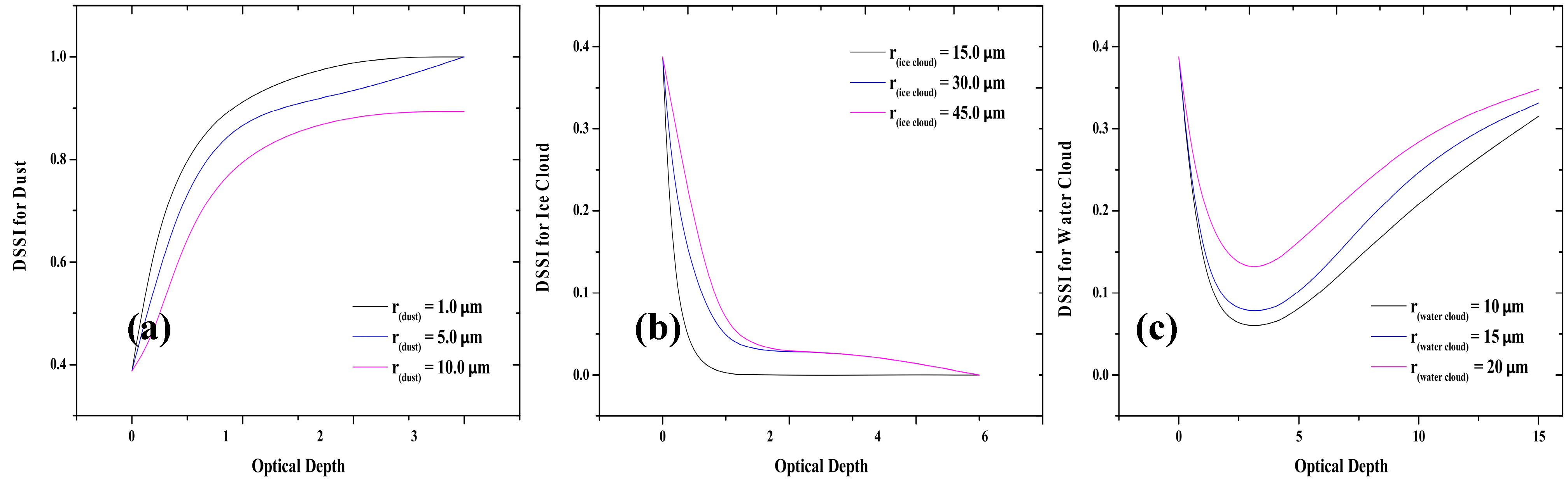
| Optical Depth | 1.0 | 3.0 | 10.0 |
| Layer Height | 3.0 km | 10.0 km | 1.0 km |
| Particle Effective Radius | 5.0 μm | 15.0 μm | 10.0 μm |
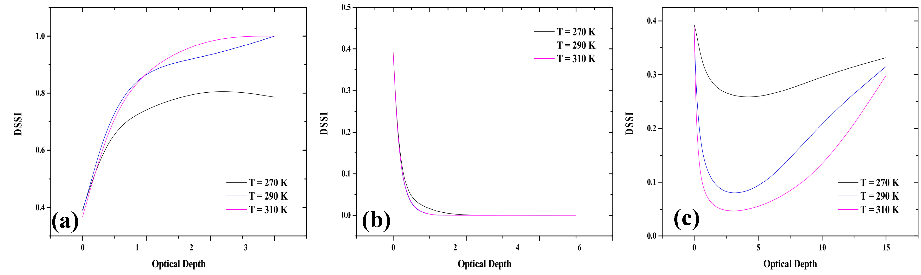
| Surface Temperature | 290.0 K | ||
| Surface Emissivity | 1.0 | ||
| Atmospheric Profile | Middle latitude winter atmospheric profile | ||
| Observation Geometry | Nadir-viewed | ||
3.2. Channel Selection

| AIRS Chanel (id) | Wavenumber (cm−1) | Wavelength (μm) | Transmittance (Middle Latitude Winter) |
|---|---|---|---|
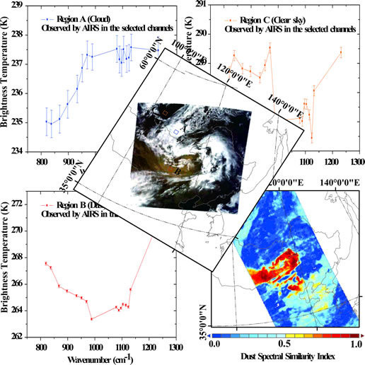
| 526 | 820.07 | 12.19 | 0.92 |
| 572 | 837.93 | 11.93 | 0.94 |
| 663 | 868.40 | 11.52 | 0.95 |
| 752 | 897.90 | 11.14 | 0.95 |
| 830 | 933.04 | 10.72 | 0.95 |
| 879 | 951.66 | 10.51 | 0.94 |
| 925 | 969.84 | 10.31 | 0.93 |
| 973 | 988.67 | 10.11 | 0.92 |
| 1152 | 1079.38 | 9.26 | 0.90 |
| 1171 | 1088.88 | 9.18 | 0.92 |
| 1186 | 1096.49 | 9.12 | 0.94 |
| 1201 | 1104.20 | 9.06 | 0.93 |
| 1222 | 1115.17 | 8.97 | 0.92 |
| 1239 | 1124.20 | 8.90 | 0.93 |
| 1254 | 1132.28 | 8.83 | 0.91 |
| 1292 | 1231.85 | 8.12 | 0.85 |
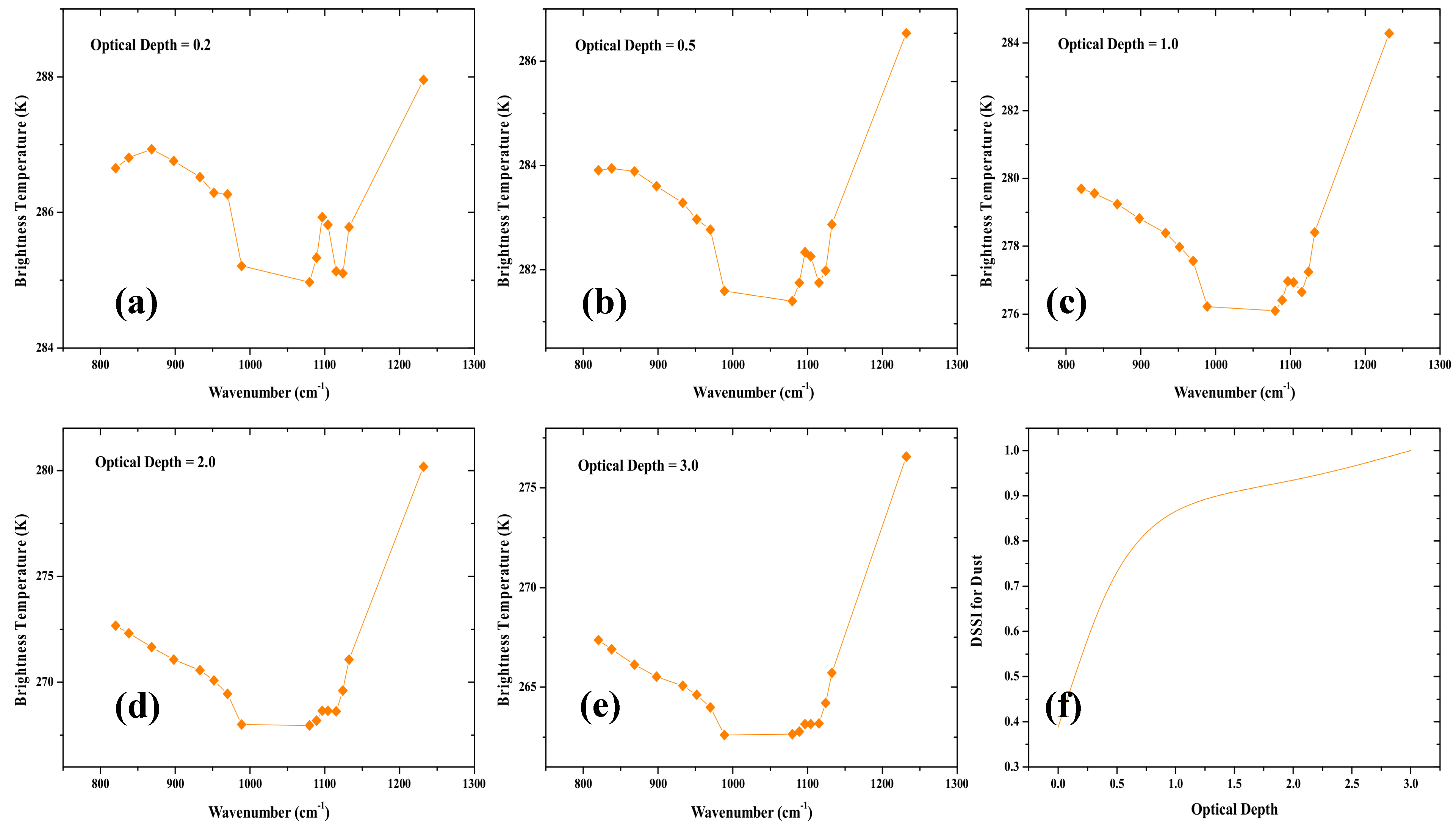
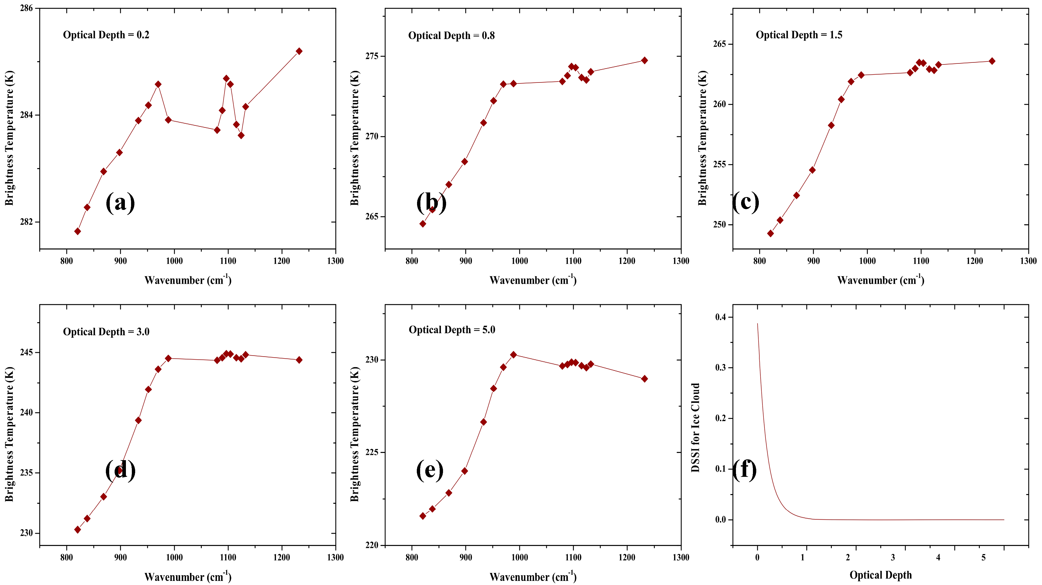
3.3. The Description of Dust Spectral Similarity Index (DSSI)
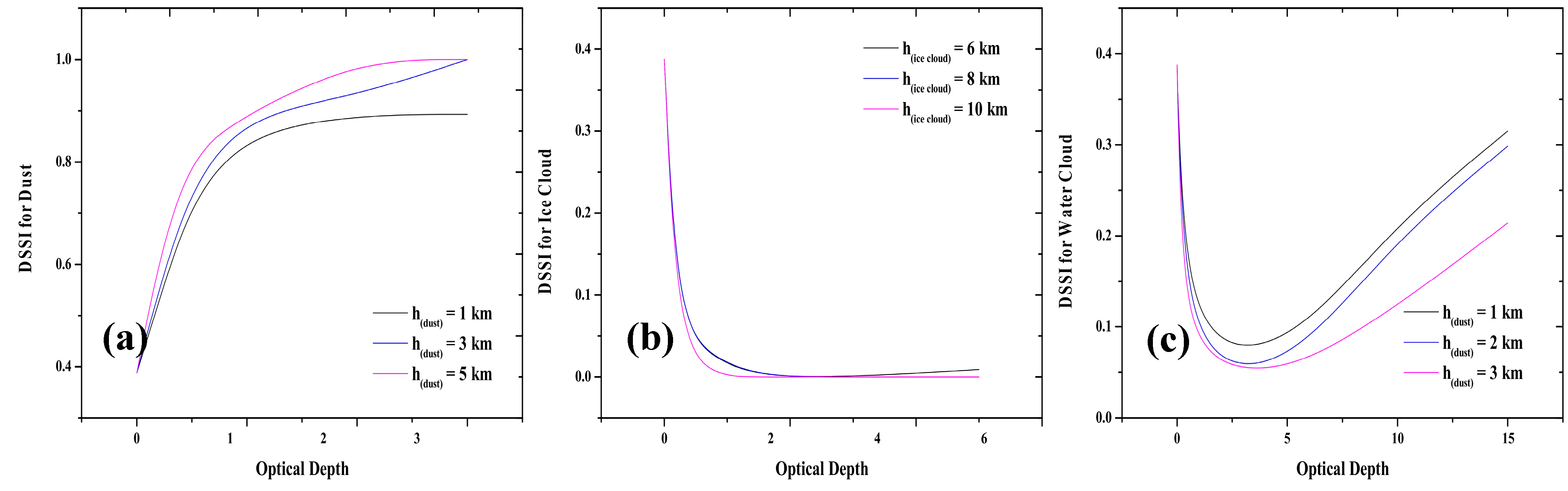
3.4. The Sensitivity Analysis of DSSI


4. Application
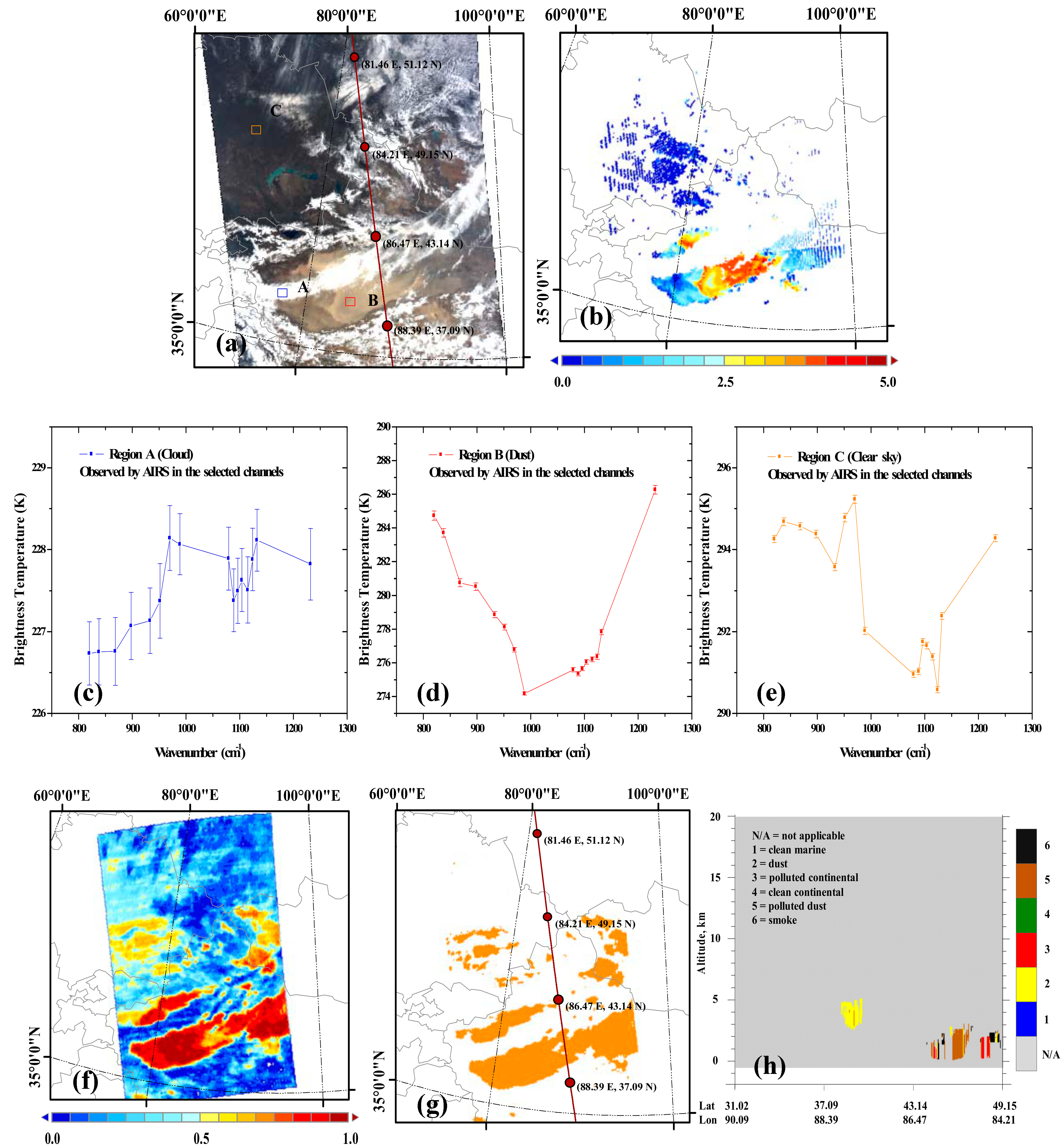
4.1. Case 1: 19 April 2008 Dust Event

4.2. Case 2: 11 May 2011 Dust Event

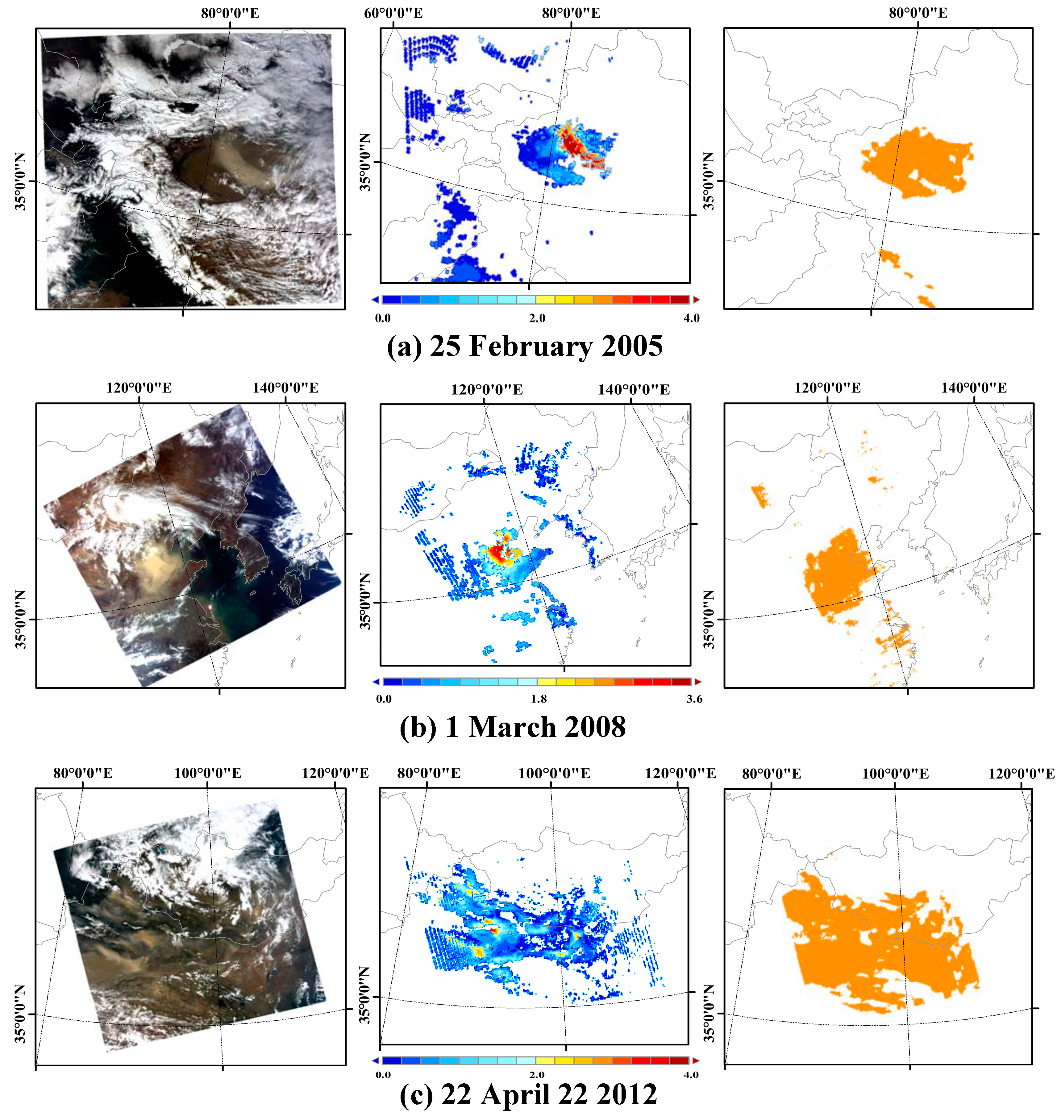
4.3. Several Other Dust Cases
5. Conclusions
Acknowledgments
Author Contributions
Conflicts of Interest
References
- Zhang, X.; Arimoto, R.; An, Z.S. Dust emission from Chinese desert sources linked to variations in atmospheric circulation. J. Geophys. Res. 1997, 102, 28041–28047. [Google Scholar] [CrossRef]
- Xuan, J; Liu, G.L.; Du, K. Dust emission inventory in Northern China. Atmos. Environ. 2000, 34, 4565–4570. [Google Scholar]
- Natsagdorj, L.; Jugder, D.; Chung, Y. Analysis of dust storms observed in Mongolia during 1937–1999. Atmos. Environ. 2003, 37, 1401–1411. [Google Scholar] [CrossRef]
- Shao, Y.; Dong, C. A review on East Asian dust storm climate, modeling and monitoring. Glob. Planet. Change 2006, 52, 1–22. [Google Scholar] [CrossRef]
- Xuan, J.; Sokolik, I. Characterization of sources and emission rates of mineral dust in Northern China. Atmos. Environ. 2002, 36, 4863–4876. [Google Scholar] [CrossRef]
- Liu, X.; Yin, Z.; Zhang, X.; Yang, X. Analyses of the spring dust storm frequency of Northern China in relation to antecedent and concurrent wind, precipitation, vegetation, and soil moisture conditions. J. Geophys. Res. 2004, 109. [Google Scholar] [CrossRef]
- Zhang, P.; Lu, N.M.; Hu, X.Q.; Dong, C.H. Identification and physical retrieval of dust storm using three MODIS thermal IR channels. Glob. Planet. Change 2006, 52, 197–206. [Google Scholar] [CrossRef]
- Wang, X.; Huang, J.; Ji, M.; Higuchi, K. Variability of East Asia dust events and their long-term trend. Atmos. Environ. 2007, 42, 3156–3165. [Google Scholar] [CrossRef]
- Kim, J. Transport routes and source regions of Asian dust observed in Korea during the past 40 years (1965–2004). Atmos. Environ. 2008, 42, 4778–4789. [Google Scholar] [CrossRef]
- Haywood, J.; Oliviler, B. Estimates of the direct and indirect radiative forcing due to tropospheric aerosol: A Review. Rev. Geophys. 2000, 38, 513–543. [Google Scholar] [CrossRef]
- Higurashi, A.; Nakajima, T. Detection of aerosol types over the East China Sea near Japan from four-channel satellite data. Geophys. Res. Lett. 2002, 29, 171–174. [Google Scholar]
- Levin, Z.; Ganor, E.; Gladstein, V. The effects of desert particles coated with sulfate on rain formation in the Eastern Mediterranean. J. Appl. Meteorol. 1996, 35, 1511–1523. [Google Scholar] [CrossRef]
- Miller, R.L.; Tegen, I. Climate response to soil dust aerosols. J. Climate 1998, 11, 3247–3267. [Google Scholar] [CrossRef]
- Sokolik, I. The spectral radiative signature of wind-blown mineral dust: Implications for remote sensing in the thermal IR region. Geophys. Res. Lett. 2002, 29. [Google Scholar] [CrossRef]
- Gu, Y.; William, I.; Gregg, J. Retrieval of mass and sizes of particles in sandstorms using two MODIS IR bands: A case study of April 7, 2001 sandstorm in China. Geophys. Res. Lett. 2003, 30. [Google Scholar] [CrossRef]
- Huang, J.; Lin, B.; Minnis, P.; Wang, T.H.; Wang, X.; Hu, Y.X.; Yi, Y.H.; Ayers, J.K. Satellite-based assessment of possible dust aerosols semi-direct effect on cloud water path over East Asia. Geophys. Res. Lett. 2006, 33. [Google Scholar] [CrossRef]
- Huang, J.; Wang, Y.; Wang, T.; Yi, Y.H. Dusty cloud radiative forcing derived from satellite data for middle latitude regions of East Asia. Process Nat. Sci. 2006, 16, 1084–1089. [Google Scholar] [CrossRef]
- Huang, J.; Minnis, B.; Lin, T.; Wang, Y.; Yi, Y.; Hu, S.; Sun-Mack; Ayers, K. Possible influences of Asian dust aerosols on cloud properties and radiative forcing observed from MODIS and CERES. Geophys. Res. Lett. 2006, 33. [Google Scholar] [CrossRef]
- Zhu, A.; Ramanathan, V.; Li, F.; Kim, D. Dust plumes over the Pacific, Indian, and Atlantic oceans: Climatology and radiative impact. J. Geophys. Res. 2007, 112. [Google Scholar] [CrossRef]
- Torres, O.; Bhartia, P.K.; Herman, J.R.; Ahmad, Z.; Gleason, J. Derivation of aerosol properties from a satellite measurement of backscattered ultraviolet radiation: Theoretical basis. J. Geophys. Res. 1998, 103, 17099–17110. [Google Scholar] [CrossRef]
- Hsu, N.C.; Si-Chee, T.; King, M.D.; Herman, J.R. Aerosol properties over bright-reflecting source regions. IEEE Geosci. Remote Sens. 2004, 42, 557–569. [Google Scholar] [CrossRef]
- Wen, S.; Rose, W.I. Retrieval of sizes and total masses of particles in volcanic clouds using AVHRR bands 4 and 5. J. Geophys. Res. 1994, 99, 5421–5431. [Google Scholar] [CrossRef]
- Ackerman, S. Remote sensing aerosols using satellite infrared observations. J. Geophys. Res. 1997, 102, 17069–17079. [Google Scholar] [CrossRef]
- Ackerman, S.A.; Strabala, K.I.; Menzel, W.P.; Frey, R.; Moeller, C.; Gumley, L.; Baum, B.A.; Seeman, S.W.; Zhang, H. Discriminating Clear-Sky from Cloud with MODIS Algorithm Theoretical Basis Document (MOD35). Available online: http://modis-atmos.gsfc.nasa.gov/_docs/atbd_mod06_old.pdf (accessed on 13 September 2014).
- Legrand, M.; Plana-Fattori, A.; N’doumé, C. Satellite detection of dust using the IR imagery of Meteosat: 1. Infrared difference dust index. J. Geophys. Res. 2001, 106, 18251–18274. [Google Scholar] [CrossRef]
- Miller, S.D. A consolidated technique for enhancing desert dust storms with MODIS. Geophys. Res. Lett. 2003, 30. [Google Scholar] [CrossRef]
- Gary, P.; Bernadette, H.; Donald, W. Improved detection of airborne volcanic ash using multispectral infrared satellite data. J. Geophys. Res. 2003, 108. [Google Scholar] [CrossRef]
- Roskovensky, J.K.; Liou, K.N. Differentiating airborne dust from cirrus clouds using MODIS data. Geophys. Res. Lett. 2005, 32. [Google Scholar] [CrossRef]
- Brindley, H.E.; Russell, J.E. Improving GERB scene identification using SEVIRI: Infrared dust detection strategy. Remote Sens. Environ. 2006, 104, 426–446. [Google Scholar] [CrossRef]
- Hansell, R.A.; Ou, S.C.; Liou, K.N.; Roskovensky, J.K.; Tsay, S.C.; Hsu, C. Simultaneous detection/separation of mineral dust and cirrus clouds using MODIS thermal infrared window data. Geophys. Res. Lett. 2007, 34. [Google Scholar] [CrossRef]
- Li, J.; Zhang, P.; Schmit, T.J.; Schmetz, J.; Menzel, W.P. Quantitative monitoring of a Saharan dust event with SEVIRI on Meteosat-8. Int. J. Remote Sens. 2007, 28, 2181–2186. [Google Scholar] [CrossRef]
- Hu, X.; Lu, N.; Zhang, P. Operational retrieval of Asian sand and dust storm from FY-2C geostationary meteorological satellite and its application to real time forecast in Asia. Atmos. Chem. Phys. 2008, 8, 1649–1659. [Google Scholar] [CrossRef]
- Klüser, L.; Schepanski, K. Remote sensing of mineral dust over land with MSG infrared channels: A new bitemporal mineral dust index. Remote Sens. Environ. 2009, 113, 1853–1867. [Google Scholar] [CrossRef] [Green Version]
- Tom, X.; Ackerman, S.; Guo, W. Dust and smoke detection for multi-channel imagers. Remote Sens. 2010, 2, 2347–2368. [Google Scholar] [CrossRef]
- Good, E.J.; Kong, X.; Embury, O.; Merchant, C.J.; Remedios, J.J. An infrared desert dust index for the along-track scanning radiometers. Remote Sens. Environ. 2012, 116, 159–176. [Google Scholar] [CrossRef]
- Gang, H.; Ping, Y.; Huang, H.; Ackerman, S.; Sokolik, I. Simulation of high-spectral-resolution infrared signature of overlapping cirrus clouds and mineral dust. Geophys. Res. Lett. 2006, 33. [Google Scholar] [CrossRef]
- Pierangelo, C.; Chédin, A.; Heilliette, S.; Jacquinet-Husson, N.; Armante, R. Dust altitude and infrared optical depth from AIRS. Atmos. Chem. Phys. 2004, 4, 1813–1822. [Google Scholar] [CrossRef]
- Peyridieu, S.; Chédin, A.; Tanré, D.; Capelle, V.; Pierangelo, C.; Lamquin, N.; Armante, R. Saharan dust infrared optical depth and altitude retrieved from AIRS: A focus over North Atlantic—Comparison to MODIS and CALIPSO. Atmos. Chem. Phys. 2010, 10, 1953–1967. [Google Scholar] [CrossRef]
- DeSouza-Machado, S.G.; Strow, L.L.; Imbiriba, B.; McCann, K.; Hoff, R.M.; Hannon, S.E.; Martins, J.V.; Tanré, D.; Deuzé, J.L.; Ducos, F.; et al. Infrared retrievals of dust using AIRS: Comparisons of optical depths and heights derived for a North African dust storm to other collocated EOS A-Train and surface observations. J. Geophys. Res. 2010, 115. [Google Scholar] [CrossRef]
- Yao, Z.G.; Li, J.; Han, H.J.; Allen, H.; Sohn, B.J.; Zhang, P. Asian dust height and infrared optical depth retrievals over land from hyperspectral longwave infrared radiances. J. Geophys. Res. 2012, 117. [Google Scholar] [CrossRef]
- Gangale, G.; Prata, A.J.; Clarisse, L. The infrared spectral signature of volcanic ash determined from high-spectral resolution satellite measurements. Remote Sens. Environ. 2010, 114, 414–425. [Google Scholar] [CrossRef]
- Barnes, W.; Pagano, T.S.; Salomonson, V.V. Prelaunch characteristics of MODIS on EOS-AM1. IEEE Trans. Geosci. Remote Sens. 1998, 36, 1088–1100. [Google Scholar] [CrossRef]
- Remer, L.A.; Kaufman, Y.J.; Tanré, D.; Mattoo, S.; Chu, D.A.; Martins, J.V.; Li, R.R.; Ichoku, C.; Levy, R.C.; Kleidman, R.G.; et al. The MODIS aerosol algorithm, products, and validation. J. Atmos. Sci. 2005, 62, 947–973. [Google Scholar] [CrossRef]
- Hess, M.; Koepke, P.; Schult, I. Optical properties of aerosols and clouds: The software package OPAC. Bull. Am. Meteorol. Soc. 1998, 79, 831–844. [Google Scholar] [CrossRef]
- Volz, F.E. Infrared refractive index of atmospheric aerosol substances. Appl. Optics 1972, 12, 564–568. [Google Scholar] [CrossRef]
- Han, H.J.; Sohn, B.J.; Huang, H.L.; Weisz, E.; Saunders, R.; Takamura, T. An improved radiance simulation for hyperspectral infrared remote sensing of Asian dust. J. Geophys. Res. 2012, 117. [Google Scholar] [CrossRef]
- Mayer, B.; Kylling, A. Technical note: The libRadtran software package for radiative transfer calculations—Description and examples of use. Atmos. Chem. Phys. 2005, 5, 1855–1877. [Google Scholar] [CrossRef]
- Baum, A.; Hymsfield, J.; Yang, P.; Bedka, S. Bulk scattering properties for the remote sensing of ice clouds. Part I: Microphysical data and models. J. Appl. Meteorol. 2005, 44, 1885–1895. [Google Scholar] [CrossRef]
- Baum, A.; Yang, P.; Heymsfield, J.; Steven, P.; Michael, D.; Hu, Y.X.; Sarah, T. Bulk scattering properties for the remote sensing of ice clouds. Part II: Narrowband models. J. Appl. Meteorol. 2005, 44, 1897–1991. [Google Scholar]
- Korolev, A.; Isaac, G.; Coberi, S.; Strapp, J.W.; Hallett, J. Microphysical characterization of mixed-phase clouds. Q. J. Roy. Meteorol. Soc. 2003, 129, 39–65. [Google Scholar] [CrossRef]
- Anderson, G.P.; Clough, S.A.; Kneizys, F.X.; Chetwynd, J.H.; Shettle, E.P. AFGL Atmospheric Constituent Profiles 0–120 km. Available online: http://oai.dtic.mil/oai/oai?verb=getRecord&metadataPrefix=html&identifier=ADA175173 (accessed on 13 September 2014).
- Wilber, A.; Kratz, D.; Cupta, S. Surface Emissivity Maps for Use in Satellite Retrievals of Longwave Radiation. Available online: http://www-cave.larc.nasa.gov/pdfs/Wilber.NASATchNote99.pdf (accessed on 13 September 2014).
© 2014 by the authors; licensee MDPI, Basel, Switzerland. This article is an open access article distributed under the terms and conditions of the Creative Commons Attribution license (http://creativecommons.org/licenses/by/4.0/).
Share and Cite
Xu, H.; Cheng, T.; Gu, X.; Yu, T.; Wu, Y.; Chen, H. New Asia Dust Storm Detection Method Based on the Thermal Infrared Spectral Signature. Remote Sens. 2015, 7, 51-71. https://doi.org/10.3390/rs70100051
Xu H, Cheng T, Gu X, Yu T, Wu Y, Chen H. New Asia Dust Storm Detection Method Based on the Thermal Infrared Spectral Signature. Remote Sensing. 2015; 7(1):51-71. https://doi.org/10.3390/rs70100051
Chicago/Turabian StyleXu, Hui, Tianhai Cheng, Xingfa Gu, Tao Yu, Yu Wu, and Hao Chen. 2015. "New Asia Dust Storm Detection Method Based on the Thermal Infrared Spectral Signature" Remote Sensing 7, no. 1: 51-71. https://doi.org/10.3390/rs70100051