
Correction of Interferometric and Vegetation Biases in the SRTMGL1 Spaceborne DEM with Hydrological Conditioning towards Improved Hydrodynamics Modeling in the Amazon Basin

 , , , and
Abstract
:
1. Introduction
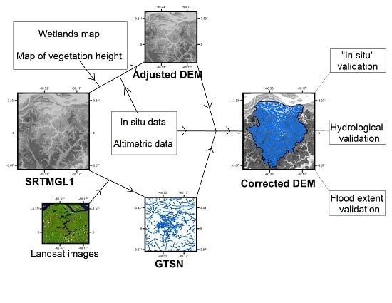
2. Method
2.1. Study Site

2.2. Data Used in the Study
2.2.1. Remote Sensing Data
SRTMGL1 and SWBD
Wetlands Map
Radar Altimetry Data
Forest Canopy Height Map
Landsat Products
2.2.2. In Situ Data
Water Level Data

Bathymetric in Situ Data
2.3. Method

2.3.1. Interferometric Bias and Vegetation Bias Correction
Interferometric Bias Correction
Vegetation Bias Correction

| Classes | ID | LW State | HW State | Elevation Constraints | Area % | Mean DEM1 Elevation (m) | Mean Tree Height (m) | Vegetation Offset (m) | Excluded % | Mean DEM_ADJ Elevations (m) |
|---|---|---|---|---|---|---|---|---|---|---|
| herbs | 11 | water | flherbs | ≤13.5 | 0.1 | 12.8 | 10.1 | 0 | 67 | 12.8 |
| 12 | herbs | water | ≥13.5 and ≤22.1 | 2.4 | 12.6 | 5.6 | 0 | 65 | 12.6 | |
| 13 | herbs | flherbs | ≥13.5 and ≤22.1 | 1.1 | 16.0 | 10.4 | 0 | 45 | 16.0 | |
| 14 | flherbs | flherbs | ≤22.1 | 3.8 | 17.8 | 9.6 | 0 | 40 | 17.8 | |
| shrub | 21 | nfshr | water | ≥13.5 and ≤22.1 | 1 | 14.1 | 6.3 | 0 | 3 | 14.1 |
| 22 | nfshr | flshr | ≥13.5 and ≤22.1 | 1.7 | 21.5 | 15.5 | 0 | 45 | 21.5 | |
| 23 | flshr | water | ≤22.1 | 0.2 | 14.1 | 13.6 | 0 | 8 | 14.1 | |
| 24 | mixed | mixed | ≤22.1 | 0.3 | 17.9 | 14.9 | 0 | 33 | 17.9 | |
| wdlands | 31 | flwd | flwd | ≤22.1 | 2.6 | 20.4 | 13.6 | 0 | 33 | 20.4 |
| forest | 41 | nffor | nffor | ≥22.1 | 4.2 | 27.5 | 18.4 | 0 | 33 | 27.5 |
| 42 | nffor | flfor | ≥13.5 and ≤22.1 | 7.9 | 27.5 | 18.2 | 9.9 | 53 | 17.9 | |
| 43 | flfor | flfor | ≤22.1 | 3.6 | 25.6 | 18.6 | 9.9 | 55 | 16.0 | |
| terra firma | 51 | nffor | nffor | ≥22.1 | 60.4 | 32.8 | 22.4 | |||
| 511 | nffor | nffor | ≥22.1 | 28.1 | 24.7 | 19.9 | 0 | 25 | 24.7 | |
| 512 | nffor | nffor | ≥22.1 | 32.2 | 39.4 | 24.5 | 14.7 | 26 | 24.7 | |
| water | 61 | water | water | ≤13.5 | 7.0 | 8.8 | 1.4 | 0 | 0 | 8.8 |
| 62 | water | water | ≤13.5 | 3.1 | 11.4 | 6.7 | 0 | 100 | - |

2.3.2. DEM Elevation Interpolation
2.3.3. Quality Assessment of the Generated DEMs
Vertical Accuracy
Stream Network Assessment
Flood Extent Assessment
3. Results and Discussion
3.1. Biases Correction
| DEM | Mean (m) | Standard Deviation (m) |
|---|---|---|
| Geoid bias | −0.3 | 0.1 |
| Interferometric bias | −2.0 | 4.1 |
| Total correction over the study area | 5.9 | 6.9 |
| Total correction restricted to the Terra Firme zone | 7.4 | 7.3 |
3.2. Accuracy Assessment
3.2.1. Vertical Accuracy Assessment

| DEM | Mean (m) | SD (m) | RMSE (m) | Roughness (m) | Outlet (Boolean) | Connectivity (Boolean) | GTSN Matching Index (%) |
|---|---|---|---|---|---|---|---|
| SRTMGL1 | −0.4 | 4.7 | 4.8 | 1.5 | 0 | 1 | 58 |
| DEM1 | 1.3 | 4.7 | 4.9 | 1.5 | 0 | 1 | 58 |
| DEM_COR | 0.1 | 1.7 | 1.7 | 0.9 | 1 | 1 | 83 |
| DEM_COR_1 | 0.9 | 4.3 | 4.4 | 1.1 | 1 | 1 | 67 |
| DEM_COR_2 | 0.4 | 1.6 | 1.6 | 0.7 | 0 | 1 | 46 |
| DEM_COR_3 | 1.9 | 4.6 | 4.9 | 0.8 | 0 | 0 | 66 |
3.2.2. Stream Network Assessment
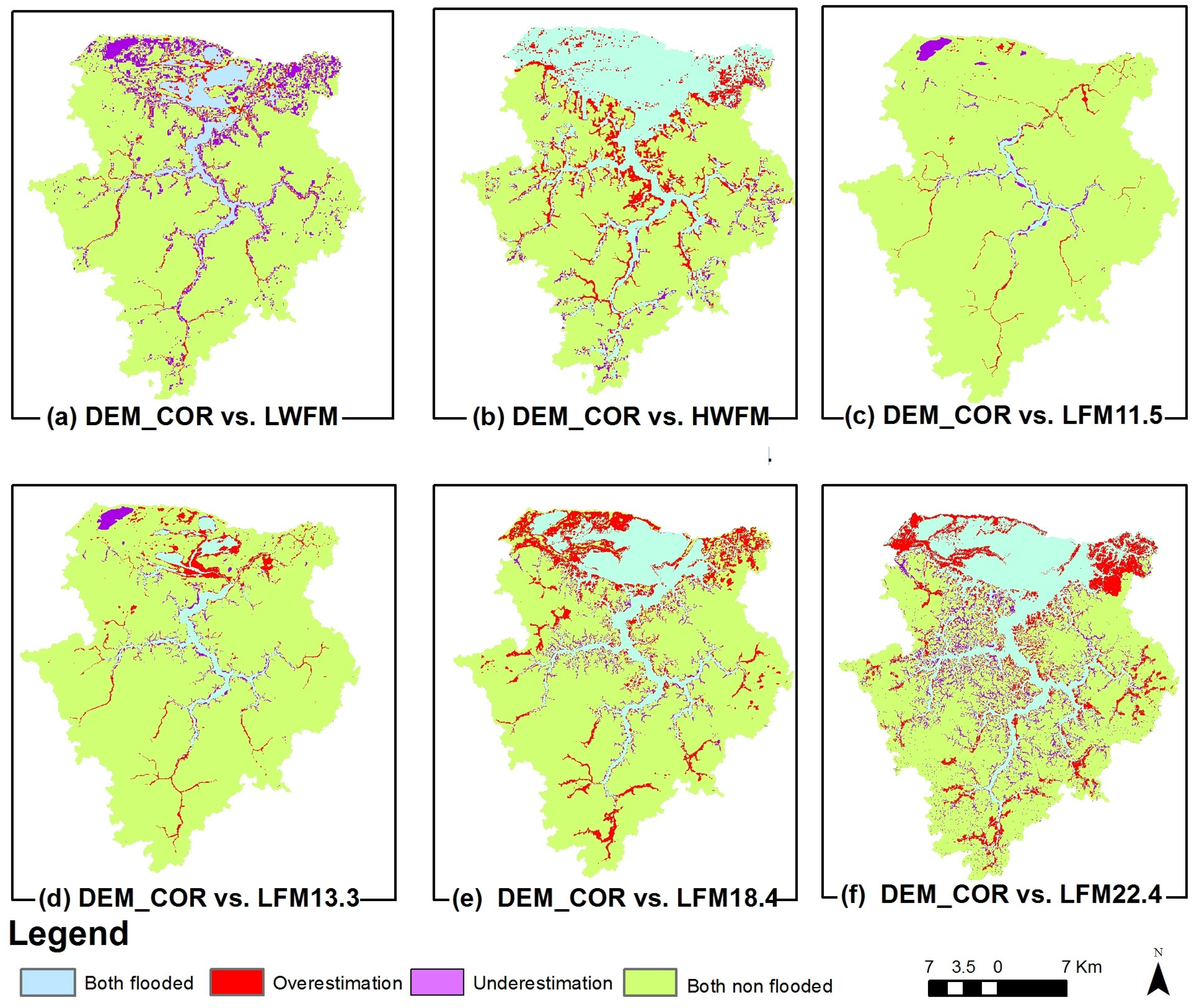
3.2.3. Flood Extent Assessment
| DEM | Landsat Images | LWFM | HWFM | ||||
|---|---|---|---|---|---|---|---|
| LFM11.5 | LFM13.3 | LFM18.4 | LFM22.5 | 13.5 m | 22.1 m | ||
| SRTMGL1 | TS | 20 | 40 | 69 | 65 | 40 | 49 |
| BIAS | −265 | −127 | −28 | −19 | −1 | −29 | |
| DEM1 | TS | 2 | 46 | 72 | 69 | 37 | 53 |
| BIAS | −27 | −63 | −17 | −4 | 27 | −1 | |
| DEM_COR | TS | 37 | 48 | 60 | 62 | 39 | 73 |
| BIAS | 3 | −28 | −43 | −17 | 37 | −24 | |
| DEM_COR_1 | TS | 26 | 45 | 75 | 71 | 37 | 53 |
| BIAS | −169 | −68 | −13 | 2 | 22 | −2 | |
| DEM_COR_2 | TS | 29 | 42 | 58 | 59 | 35 | 75 |
| BIAS | 51 | 9 | −35 | −11 | 53 | −18 | |
| DEM_COR_3 | TS | 15 | 44 | 60 | 62 | 42 | 75 |
| BIAS | −84 | −55 | −34 | −12 | 27 | −18 | |


3.3. Implications for Morphological and Hydrological Characteristics
| Drainage Network | Watershed(km2) | LW Flooded Area (km2) | HW Flooded Area (km2) | Longest Flow Path (km) | Slope (cm/km) | Concentration Time (h) |
|---|---|---|---|---|---|---|
| SRTMGL1 | 795 | 88 | 397 | 68 | 88 | 26 |
| DEM1 | 805 | 31 | 309 | 69 | 87 | 26 |
| DEM_COR | 786 | 23 | 391 | 96 | 31 | 50 |
| DEM_COR_1 | 737 | 46 | 304 | 94 | 59 | 38 |
| DEM_COR_2 | 854 | 10 | 406 | 83 | 36 | 42 |
| DEM_COR_3 | 788 | 44 | 384 | 81 | 35 | 41 |

3.4. Usefulness of Bathymetric Data in the Correction Process
4. Conclusions
Acknowledgments
Author Contributions
Conflicts of Interest
References
- Costanza, R.; Arge, R.; de Groot, R.; Farberk, S.; Grasso, M.; Hannon, B.; Limburg, K.; Naeem, S.; Neill, R.V.O.; Paruelo, J.; et al. The value of the world’s ecosystem services and natural capital. Nature 1997, 387, 253–260. [Google Scholar] [CrossRef]
- Mitsch, W.J.; Gosselink, J.G. Wetlands, 4th ed.; John Wiley and Sons: Charlottesville, VA, USA, 2007. [Google Scholar]
- Melack, J.M.; Hess, L. Remote sensing of the distribution and extent of wetlands in the Amazon basin. In Amazonian Floodplain Forests: Ecophysiology, Ecology, Biodiversity and Sustainable Management; Junk, W.J., Piedade, M., Eds.; Ecological Studies-Springer: Berlin, Germany, 2011; pp. 1–28. [Google Scholar]
- Paiva, R.C.D.; Collischonn, W.; Tucci, C.E.M. Large scale hydrologic and hydrodynamic modeling using limited data and a GIS based approach. J. Hydrol. 2011, 406, 170–181. [Google Scholar] [CrossRef]
- Yamazaki, D.; Kanae, S.; Kim, H.; Oki, T. A physically based description of floodplain inundation dynamics in a global river routing model. Water Resour. Res. 2011, 47, W04051. [Google Scholar] [CrossRef]
- Mangiarotti, S.; Martinez, J.M.; Bonnet, M.P.; Buarque, D.C.; Filizola, N.; Mazzega, P. Discharge and suspended sediment flux estimated along the mainstream of the Amazon and the Madeira Rivers (from in situ and MODIS Satellite Data). Int. J. Appl. Earth Obs. Geoinform. 2013, 21, 341–355. [Google Scholar] [CrossRef] [Green Version]
- Bourgoin, L.M.; Bonnet, M.P.; Martinez, J.-M.; Kosuth, P.; Cochonneau, G.; Moreira-Turcq, P.; Guyot, J.L.; Vauchel, P.; Filizola, N.; Seyler, P. Temporal dynamics of water and sediment exchanges between the Curuaí floodplain and the Amazon River, Brazil. J. Hydrol. 2007, 335, 140–156. [Google Scholar] [CrossRef]
- Dunne, T.; Mertes, L.A.K.; Meade, R.H.; Richey, J.E.; Forsberg, B.R. Exchanges of sediment between the flood plain and channel of the Amazon River in Brazil. Geol. Soc. Am. Bull. 1998, 110, 450–467. [Google Scholar] [CrossRef]
- Moreira-Turcq, P.; Bonnet, M.P.; Amorim, M.; Bernardes, M.; Lagane, C.; Maurice-Bourgoin, L.; Perez, M.; Seyler, P. Seasonal variability in concentration, composition, age, and fluxes of particulate organic carbon exchanged between the floodplain and Amazon River. Glob. Biogeochem. Cycles 2013, 27, 119–130. [Google Scholar] [CrossRef]
- Abril, G.; Martinez, J.; Artigas, L.; Moreira-Turcq, P.; Benedetti, F.; Vidal, L.; Meziane, T.; Kim, J.; Bernardes, M.C.; Savoye, N.; et al. Amazon River carbon dioxide outgassing fuelled by wetlands. Nature 2014, 505, 395–398. [Google Scholar] [CrossRef] [PubMed]
- Junk, W. General Aspects of Floodplain Ecology with Special Reference to Amazonian Floodplains; Junk, W.J., Ed.; Springer Verlag: Berlin, Germany, 1997; Volume 126. [Google Scholar]
- Junk, W.; Bayley, P.B.; Sparks, R.E. The flood pulse concept in river-floodplain systems. Can. Spec. Publ. Fish. Aquat. Sci. 1989, 106, 110–127. [Google Scholar]
- Bonnet, M.P.; Barros, W.; Martinez, J.M.; Seyler, F.; Moreira-Turcq, P.; Cochonneau, G.; Melack, J.M.; Boaventura, G.R.; Maurice-Bourgoin, L.; Leon, J.G.; et al. Floodplain hydrology in an Amazon floodplain lake (Lago Grande de Curuai). J. Hydrol. 2008, 349, 18–30. [Google Scholar] [CrossRef] [Green Version]
- Lesack, L.F.W.; Melack, J.M. Flooding hydrology and mixture dynamics of lake water derived from multiple sources in an Amazon floodplain lake. Water Resour. Res. 1995, 31, 329–345. [Google Scholar] [CrossRef]
- Rudorff, C.D.M.; Melack, J.M.; Bates, P. Flooding dynamics on the lower Amazon floodplain: 2. Seasonal and interannual hydrological variability. Water Resour. Res. 2014, 50, 635–649. [Google Scholar] [CrossRef]
- Melack, J.M.; Forsberg, B.R. Biogeochemistry of Amazon floodplain lakes and associated wetlands. In Biogeochemistry of the Amazon Basin; McClain, M.E., Victoria, R.L., Richey, J.E., Eds.; Oxford University Press: New York, NY, USA, 2001; pp. 235–276. [Google Scholar]
- Mertes, L.A.K. Documentation and significance of the perirheic zone on inundated floodplains. Water Resour. Res. 1997, 33, 1749–1762. [Google Scholar] [CrossRef]
- Castello, L.; Mcgrath, D.G.; Hess, L.; Coe, M.T.; Lefebvre, P.; Petry, P.; Macedo, M.N.; Renó, V.F.; Arantes, C.C. The vulnerability of Amazon freshwater ecosystems. Conserv. Lett. 2013, 6, 217–229. [Google Scholar] [CrossRef]
- Gloor, M.; Brienen, R.J.W.; Galbraith, D.; Feldpausch, T.R.; Schöngart, J.; Guyot, J.L.; Lloyd, J.; Espinoza, J.C.; Phillips, O.L. Intensification of the Amazon hydrological cycle over the last two decades. Geophys. Res. Lett. 2013, 40, 1729–1733. [Google Scholar] [CrossRef]
- Bates, P.; de Roo, A.P. A simple raster-based model for flood inundation simulation. J. Hydrol. 2000, 236, 54–77. [Google Scholar] [CrossRef]
- Hunter, N.M.; Horritt, M.; Bates, P.; Wilson, M.; Werner, M.G.F. An adaptive time step solution for raster-based storage cell modelling of floodplain inundation. Adv. Water Resour. 2005, 28, 975–991. [Google Scholar] [CrossRef]
- Bates, P.; Horritt, M.S.; Fewtrell, T.J. A simple inertial formulation of the shallow water equations for efficient two-dimensional flood inundation modelling. J. Hydrol. 2010, 387, 33–45. [Google Scholar] [CrossRef]
- De Almeida, G.A.M.; Bates, P.; Freer, J.E.; Souvignet, M. Improving the stability of a simple formulation of the shallow water equations for 2-D flood modeling. Water Resour. Res. 2012, 48, 1–14. [Google Scholar] [CrossRef]
- Yamazaki, D.; de Almeida, G.A.M.; Bates, P. Improving computational efficiency in global river models by implementing the local inertial flow equation and a vector-based river network map. Water Resour. Res. 2013, 49, 7221–7235. [Google Scholar] [CrossRef]
- Baugh, C.; Bates, P.; Schumann, G.; Trigg, M. SRTM vegetation removal and hydrodynamic modeling accuracy. Water Resour. Res. 2013, 49, 5276–5289. [Google Scholar] [CrossRef]
- Rudorff, C.D.M.; Melack, J.M.; Bates, P. Flooding dynamics on the lower Amazon floodplain: 1. Hydraulic controls on water elevation, inundation extent, and river-floodplain discharge. Water Resour. Res. 2014, 50, 619–634. [Google Scholar] [CrossRef]
- Wilson, M.; Bates, P.; Alsdorf, D.E.; Forsberg, B.R.; Horritt, M.S.; Melack, J.M.; Frappart, F.; Famiglietti, J. Modeling large-scale inundation of Amazonian seasonally flooded wetlands. Geophys. Res. Lett. 2007, 34, L15404. [Google Scholar] [CrossRef]
- Alsdorf, D.E.; Bates, P.; Melack, J.M.; Wilson, M.; Dunne, T. Spatial and temporal complexity of the Amazon flood measured from space. Geophys. Res. Lett. 2007, 34, L08402. [Google Scholar] [CrossRef]
- Sanders, B.F. Evaluation of on-line DEMs for flood inundation modeling. Adv. Water Resour. 2007, 30, 1831–1843. [Google Scholar] [CrossRef]
- Farr, T.G.; Rosen, P.A.; Caro, E.; Crippen, R.; Duren, R.; Hensley, S.; Kobrick, M.; Paller, M.; Rodriguez, E.; Roth, L.; et al. The shuttle radar topography mission. Rev. Geophys. 2007, 45, 361–364. [Google Scholar] [CrossRef]
- Rodriguez, E.; Morris, C.C.; Belz, J.J. A global assessment of the SRTM performance. Photogramm. Eng. Remote Sens. 2006, 72, 249–260. [Google Scholar] [CrossRef]
- Walker, W.; Kellndorfer, J.M.; Pierce, L. Quality assessment of SRTM C- and X-band interferometric data: Implications for the retrieval of vegetation canopy height. Remote Sens. Environ. 2007, 106, 428–448. [Google Scholar] [CrossRef]
- Brown, G.; Sarabandi, K.; Pierce, L. Model-based estimation of forest canopy height in red and austrian pine stands using shuttle radar topography mission and ancillary data: A proof-of-concept study. IEEE Trans. Geosci. Remote Sens. 2010, 48, 1105–1118. [Google Scholar] [CrossRef]
- Carabajal, C.C.; Harding, D. SRTM C-Band and ICESat laser altimetry elevation comparisons as a function of tree cover and relief. Photogramm. Eng. Remote Sens. 2006, 72, 287–298. [Google Scholar] [CrossRef]
- Coe, M.T.; Costa, M.H.; Howard, E.A. Simulating the surface waters of the Amazon River basin: Impacts of new river geomorphic and flow parameterizations. Hydrol. Process. 2007, 22, 2542–2553. [Google Scholar] [CrossRef]
- Paiva, R.C.D.; Collischonn, W.; Buarque, D.C. Validation of a full hydrodynamic model for large-scale hydrologic modelling in the Amazon. Hydrol. Process. 2011, 27, 333–346. [Google Scholar] [CrossRef]
- Wittmann, F.; Junk, W.; Piedade, M.T.F. The várzea forests in Amazonia: Flooding and the highly dynamic geomorphology interact with natural forest succession. For. Ecol. Manag. 2004, 196, 199–212. [Google Scholar] [CrossRef]
- Hess, L.; Melack, J.M.; Novo, E.M.L.M.; Barbosa, C.C.F.; Gastil, M. Dual-season mapping of wetland inundation and vegetation for the central Amazon basin. Remote Sens. Environ. 2003, 87, 404–428. [Google Scholar] [CrossRef]
- Simard, M.; Pinto, N.; Fisher, J.; Baccini, A. Mapping forest canopy height globally with spaceborne lidar. J. Geophys. Res. 2011, 116, G04021. [Google Scholar] [CrossRef]
- Yamazaki, D.; Baugh, C.; Bates, P.; Kanae, S.; Alsdorf, D.E.; Oki, T. Adjustment of a spaceborne DEM for use in floodplain hydrodynamic modeling. J. Hydrol. 2012, 436–437, 81–91. [Google Scholar] [CrossRef]
- Hutchinson, M.F. Anudem Version 5.3 User Guide 2011; Australian National University: Canberra, Australia, 2011. [Google Scholar]
- Hutchinson, M.F.; Gallant, J.C. Digital Elevation Models and Representation of Terrain Shape. In Terrain Analysis: Principles and Applications; John Wiley and Sons: Charlottesville, VA, USA, 2000; pp. 29–50. [Google Scholar]
- Sioli, H. The Amazon and its main afluents: Hydrography, morphology of the river courses and river types. In The Amazon Liminology and Landscape Ecology of a Mighty Tropical River and Its Basin; Springer: Amsterdam, The Netherlands, 1984; pp. 127–165. [Google Scholar]
- Bonnet, M.P.; Lamback, B.; Boaventura, G.R.; Oliveira, E. Impact of the 2009 Exceptional Flood on the Flood Plain of the Solimões River; IAHS-AISH Publication: Wallingford, CT, USA, 2011. [Google Scholar]
- NASA’s Earth Observing System Data and Information System. Available online: http://reverb.echo.nasa.gov/ (accessed on 1 September 2014).
- Pavlis, N.K.; Holmes, S.A.; Kenyon, S.C.; Factor, J.K. Erratum: Correction to the development and evaluation of the earth gravitational model 2008 (EGM2008). J. Geophys. Res. Solid Earth 2013, 118. [Google Scholar] [CrossRef]
- NGA Programs relative to EGM08. Available online: http://earthinfo.nga.mil/GandG/wgs84/gravitymod/ (accessed on 1 September 2014).
- Satge, F.; Bonnet, M.P.; Calmant, S.; Cretaux, J.F. Accuracy assessment of SRTM V4 and ASTER GDEM V2 over the 2 altiplano’s watershed using ICESat/GLAS data. Int. J. Remote Sens. 2015, 36, 465–488. [Google Scholar] [CrossRef]
- Esri, A. ESRI shapefile technical description. Comput. Stat. 1998, 16, 370–371. [Google Scholar]
- Lehner, B.; Verdin, K.L.; Jarvis, A. HydroSHEDS Technical Documentation v1.0; World Wildlife Fund US: Washington, DC, USA, 2006; pp. 1–27. [Google Scholar]
- Koblinsky, C.; Clarke, R.T. Measurement of river level variations with satellite altimetry. Water Resour. Res. 1993, 29, 1839–1848. [Google Scholar] [CrossRef]
- Birkett, C.M.; Mertes, L.A.K.; Dunne, T.; Costa, M.H.; Jasinski, M.J. Surface water dynamics in the Amazon Basin: Application of satellite radar altimetry. J. Geophys. Res. Atmos. 2002, 107, LBA-26. [Google Scholar] [CrossRef]
- Roux, E.; Santos da Silva, J.; Cesar Vieira Getirana, A.; Bonnet, M.P.; Calmant, S.; Seyler, F.; Martinez, J.-M.M.; Getirana, A. Producing time series of river water height by means of satellite radar altimetry—A comparative study. Hydrol. Sci. J. 2010, 55, 104–120. [Google Scholar] [CrossRef]
- Alsdorf, D.E.; Rodriguez, E.; Lettenmaier, D.P. Measuring surface water from space. Rev. Geophys. 2007, 45, 1–24. [Google Scholar] [CrossRef]
- Calmant, S.; Seyler, F. Continental surface waters from satellite altimetry. Comptes Rendus Geosci. 2006, 338, 1113–1122. [Google Scholar] [CrossRef]
- Santos da Silva, J.; Calmant, S.; Seyler, F.; Rotunno Filho, O.C.; Cochonneau, G.; Mansur, W.J.J. Water levels in the Amazon basin derived from the ERS 2 and ENVISAT radar altimetry missions. Remote Sens. Environ. 2010, 114, 2160–2181. [Google Scholar] [CrossRef]
- Frappart, F.; Calmant, S.; Cauhope, M.; Seyler, F.; Cazenave, A. Preliminary results of ENVISAT RA-2-derived water levels validation over the Amazon basin. Remote Sens. Environ. 2006, 100, 252–264. [Google Scholar] [CrossRef] [Green Version]
- CTOH. Available online: http://www.legos.obs-mip.fr/en/soa/hydrologie/hydroweb/ (accessed on 1 September 2014).
- Santos da Silva, J. Application de l Altimetrie Spatiale a l etude des Processus Hydrologique dans les zones Humides du Bassin Amazonnien. Ph.D. Thesis, Université Paul Sabatier-Toulouse III, Toulouse, France, June 2010. [Google Scholar]
- Urban, T.J.; Schutz, B.E.; Neuenschwander, A.L. A survey of ICESat coastal altimetry applications: Continental coast, open ocean island, and Inland River. Terr. Atmos. Ocean. Sci. 2008, 19, 1–19. [Google Scholar] [CrossRef]
- Zwally, H.J.; Schutz, B.; Abdalati, W.; Abshire, J.; Bentley, C.; Brenner, A.; Bufton, J.; Dezio, J.; Hancock, D.; Harding, D.; et al. ICESat’s laser measurements of polar ice, atmosphere, ocean, and land. J. Geodyn. 2002, 34, 405–445. [Google Scholar] [CrossRef]
- Schutz, B.; Zwally, H.J.; Shuman, C.A.; Hancock, D.; DiMarzio, J.P. Overview of the ICESat mission. Geophys. Res. Lett. 2005, 32, 1–4. [Google Scholar] [CrossRef]
- JPL Active Optical Sensing Group. Available online: http://lidarradar.jpl.nasa.gov/ (accessed on 1 September 2014).
- Woodcock, C.; Allen, R.; Anderson, M.; Belward, A.; Bindschadler, R.; Cohen, W.; Gao, F. Free Access to Landsat Imagery. Science 2008, 320, 1011–1011. [Google Scholar] [CrossRef] [PubMed]
- USGS Landsatlook Viewer. Available online: http://landsatlook.usgs.gov/ (accessed on 1 September 2014).
- ANA. Available online: http://hidroweb.ana.gov.br/ (accessed on 1 September 2014).
- Santos da Silva, J.; Calmant, S.; Seyler, F.; Moreira, D.M.; Oliveira, D.; Monteiro, A. Radar altimetry aids managing gauge networks. Water Resour. Manag. 2014, 28, 587–603. [Google Scholar] [CrossRef]
- Jenson, S.K.; Domingue, J.O. Extracting topographic structure from digital elevation data for geographic information system analysis. Photogramm. Eng. Remote Sens. 1988, 54, 1593–1600. [Google Scholar]
- Toivonen, T.; Mäki, S.; Kalliola, R. The riverscape of Western Amazonia—A quantitative approach to the fluvial biogeography of the region. J. Biogeogr. 2007, 34, 1374–1387. [Google Scholar] [CrossRef]
- Horritt, M.S.; Bates, P. Effects of spatial resolution on a raster based model of flood flow. J. Hydrol. 2001, 253, 239–249. [Google Scholar] [CrossRef]
- Wilks, D.S. Statistical Methods in the Atmospheric Sciences; Academic Press: New York, NY, USA, 2006; Volume 14. [Google Scholar]
- Wittmann, F.; Anhuf, D.; Funk, W.J. Tree species distribution and community structure of central Amazonian várzea forests by remote-sensing techniques. J. Trop. Ecol. 2002, 18, 805–820. [Google Scholar] [CrossRef]
- Schöngart, J.; Wittmann, F.; Worbes, M. Biomass and net primary production of central Amazonian floodplain forests. In Amazonian Floodplain Forests Ecophysiology Biodiversity and Sustainable Management; Springer: Amsterdam, The Netherlands, 2010; Volume 210, pp. 347–388. [Google Scholar]
- Collischonn, W.; Allasia, D.; da Silva, B.C.; Tucci, C.E.M. The MGB-IPH model for large-scale rainfall-Runoff modelling. Hydrol. Sci. J. 2007, 52, 878–895. [Google Scholar] [CrossRef]
- Beighley, R.E.; Eggert, K.G.; Dunne, T.; He, Y.; Gummadi, V.; Verdin, K.L. Simulating hydrologic and hydraulic processes throughout the Amazon River Basin. Hydrol. Process. 2009, 23, 1221–1235. [Google Scholar] [CrossRef]
- Williams, M.R.; Melack, J.M. Solute export from forested and partially deforested catchments in the central amazon. Biogeochemistry 1997, 38, 67–102. [Google Scholar] [CrossRef]
- Pfeffer, J.; Seyler, F.; Bonnet, M.P.; Calmant, S.; Frappart, F.; Papa, F.; Paiva, R.C.D.; Satge, F.; Silva, J. Low-water maps of the groundwater table in the central Amazon by satellite altimetry. Geophys. Res. Lett. 2014, 14, 1981–1987. [Google Scholar] [CrossRef]
© 2015 by the authors; licensee MDPI, Basel, Switzerland. This article is an open access article distributed under the terms and conditions of the Creative Commons by Attribution (CC-BY) license (http://creativecommons.org/licenses/by/4.0/).
Share and Cite
Pinel, S.; Bonnet, M.-P.; Santos Da Silva, J.; Moreira, D.; Calmant, S.; Satgé, F.; Seyler, F. Correction of Interferometric and Vegetation Biases in the SRTMGL1 Spaceborne DEM with Hydrological Conditioning towards Improved Hydrodynamics Modeling in the Amazon Basin. Remote Sens. 2015, 7, 16108-16130. https://doi.org/10.3390/rs71215822
Pinel S, Bonnet M-P, Santos Da Silva J, Moreira D, Calmant S, Satgé F, Seyler F. Correction of Interferometric and Vegetation Biases in the SRTMGL1 Spaceborne DEM with Hydrological Conditioning towards Improved Hydrodynamics Modeling in the Amazon Basin. Remote Sensing. 2015; 7(12):16108-16130. https://doi.org/10.3390/rs71215822
Chicago/Turabian StylePinel, Sebastien, Marie-Paule Bonnet, Joecila Santos Da Silva, Daniel Moreira, Stephane Calmant, Fredéric Satgé, and Fredérique Seyler. 2015. "Correction of Interferometric and Vegetation Biases in the SRTMGL1 Spaceborne DEM with Hydrological Conditioning towards Improved Hydrodynamics Modeling in the Amazon Basin" Remote Sensing 7, no. 12: 16108-16130. https://doi.org/10.3390/rs71215822