Article

Improved POLSAR Image Classification by the Use of Multi-Feature Combination

1
College of Resource Environment and Tourism, Capital Normal University, Beijing 100048, China
2
Department of Geography, University of South Carolina, Columbia, SC 29208, USA
*
Author to whom correspondence should be addressed.
Remote Sens. 2015, 7(4), 4157-4177; https://doi.org/10.3390/rs70404157
Submission received: 29 December 2014 / Revised: 26 March 2015 / Accepted: 1 April 2015 / Published: 8 April 2015

Abstract

:
Polarimetric SAR (POLSAR) provides a rich set of information about objects on land surfaces. However, not all information works on land surface classification. This study proposes a new, integrated algorithm for optimal urban classification using POLSAR data. Both polarimetric decomposition and time-frequency (TF) decomposition were used to mine the hidden information of objects in POLSAR data, which was then applied in the C5.0 decision tree algorithm for optimal feature selection and classification. Using a NASA/JPL AIRSAR POLSAR scene as an example, the overall accuracy and kappa coefficient of the proposed method reached 91.17% and 0.90 in the L-band, much higher than those achieved by the commonly applied Wishart supervised classification that were 45.65% and 0.41. Meantime, the overall accuracy of the proposed method performed well in both C- and P-bands. Polarimetric decomposition and TF decomposition all proved useful in the process. TF information played a great role in delineation between urban/built-up areas and vegetation. Three polarimetric features (entropy, Shannon entropy, T11 Coherency Matrix element) and one TF feature (HH intensity of coherence) were found most helpful in urban areas classification. This study indicates that the integrated use of polarimetric decomposition and TF decomposition of POLSAR data may provide improved feature extraction in heterogeneous urban areas.

Graphical Abstract

1. Introduction

Terrain and land-use classification is an important component of synthetic aperture radar (SAR) image application. SAR data in early years were often collected at a single frequency and pre-determined polarization (H or V), which precluded the separation and mapping of terrain classes due to limited information obtained by these systems [1]. Polarimetric SAR (POLSAR) submits and receives fully polarized radar signals, containing more information on land surfaces than conventional single- or dual-polarization SAR systems [2]. It is reported in past studies that terrain surfaces can be classified more accurately from POLSAR data [3,4,5,6]. The POLSAR image classification has become an important research topic since POLSAR images from ENVISAT ASAR, ALOS PALSAR, TerraSAR-X, Cosmos sky-med and RADARSAT-2 are made publicly available.
A group of methods have been proposed for classifying POLSAR imagery, which can be divided into three schemes. The first classification scheme is based on polarimetric decomposition theory [2]. The decomposed polarimetric parameters are related to physical properties of natural media and thus help in identifying terrain classes. Example classifiers in this scheme include the Entropy/Anisotropy/Alpha [7], Freeman 3-component decomposition [8], and Yamaguchi 4-component decomposition [9]. The second classification scheme incorporates statistical data such as the polarimetric covariance matrix and the distance between an unknown pixel and a clustering center in feature space [10,11]. These statistical measures have been commonly applied in regular supervised or unsupervised (e.g., ISODATA) classification. The third classification scheme adopts the so-called integrated approach, which combines the abovementioned polarimetric decomposition and statistical classification. A representative example is the Entropy/Alpha-Wishart classifier [12]. In this approach, the polarimetric data are first initialized by the entropy/alpha decomposition, and the maximum likelihood classification is applied to extract the best-fit complex Wishart distribution [13] of the training samples. Besides the polarimetric decomposition information, this classification scheme can be improved by introducing additional features such as polarimetric interferometric SAR (PolInSAR) [14] and multi-polarization textural information [15,16,17].
Classifiers can be broadly divided into two categories: statistical clustering [18] and machine learning [19]. A well-recognized example of statistical classifier is the complex Wishart classifier [11], a pixel-based maximum likelihood classifier based on a complex Wishart distribution of the polarimetric coherency matrix [20]. It requires that the distribution of ground features follow a normal probability distribution function. The complex distribution of ground features, especially for those in high-resolution POLSAR data, often violates this premise and leads to poor classification results [21]. Example machine learning classifiers include support vector machine (SVM), C5.0 decision tree algorithm, neural network algorithm and ensemble learning methods [19,22], each with distinctive characteristics. Among these, however, the most effective method for classifying POLSAR data is not clear. Another concern in POLSAR image classification is the feature selection. Whether using the statistical clustering or machine learning, feature selection is a critical issue. Numerous features can be extracted from POLSAR data, some of which have been widely applied such as radiometric information and full-polarization decomposition features. Recently, new polarimetric features such as time-frequency (TF) decomposition [23] have been extracted but have yet to be applied in classification. Whether these newly-identified features are useful in classifying POLSAR data is uncertain.
In this study, we explored various processes of feature and classifier selection and proposed a new method for classifying POLSAR data by integrating polarimetric decomposition and TF decomposition. By evaluating the input features, the C5.0 decision tree algorithm [24] efficiently selects the most important features and determines the splits for final tree construction. The effectiveness and stability of these algorithms were demonstrated in experiments on an example C-, L- and P-band NASA/JPL AIRSAR dataset.

2. Study Site and Dataset

The study area is located in San Francisco, CA, USA. As shown in the Pauli-color coded L-band polarimetric image (Figure 1), it covers both natural targets and urban areas with differently oriented buildings. Common ground covers include sea surfaces, forests, buildings, grass fields, bare grounds, parking lots, and sand surfaces. In Pauli-color coded scheme, red, green and blue are Pauli-color coded as |HH – VV|, |HV|, and |HH + VV|, respectively. In this composition, predominantly surface-scattering objects have bluish tones, double bounce reflections in red and volume scatterers in green.
Figure 1. Study area in San Francisco and the AIRSAR L-band polarimetric image with Pauli color coding (Red: |HH – VV|, Green: |HV|, Blue: |HH + VV|).
Remotesensing 07 04157 g001
The POLSAR data were the Airborne Synthetic Aperture Radar (AIRSAR) fully polarimetric C-, L-, and P-band images downloaded from NASA Jet Propulsion Laboratory (JPL) [25]. The images were acquired on 15 July 1994. The look angle ranges from 21.5° at near range to 71.4° at far range. The ground spatial resolution is about 6.6 m in the range direction and 9.3 m in the azimuthal direction. Before image analysis, this POLSAR dataset was filtered using the 5 × 5 refined Lee POLSAR speckle filter [26]. It effectively preserves polarimetric information and retains subtle details while reducing the speckle effect in homogeneous areas.
A set of 12 classes were selected to represent land covers in the image: ocean at far range (FO), ocean at near range (NO), ocean centralized between far and near range (MO), lake (LK), dense forest (DF), trees (TS), grass (GS), bare land (BL), road (RD), orthogonal building (OB), non-orthogonal building (NB) and shadow (SD). Ocean surfaces were divided into far, central and near ocean areas according to their locations along the range direction because radar backscattering on ocean surfaces is affected by incident angles. In addition, classification accuracy of buildings is affected by the orientation of the building relative to the radar line of sight. Thus, buildings were divided into orthogonal and non-orthogonal classes.
By visually interpreting these polarimetric data and referring to Google Earth images, we randomly extracted polygons of the 12 classes (31,929 pixels) of the study area. In order to explain the polygons clearly, the distribution of the samples is shown on the span image in Figure 2. These pixels were then randomly divided into training and validation samples (Table 1). These samples were used for training and accuracy assessment of the POLSAR classification.
Figure 2. The distribution of the samples shown on the span image.
Remotesensing 07 04157 g002
Table 1. Number of Pixels Allocated to Training and Validation Samples in Image Classification.
ClassAbbr.Training (Pixels)Validation (Pixels)
far OceanFO22102204
near oceanNO21192106
middle oceanMO20001948
lakeLK338271
dense forestDF850884
treesTS10111128
grassGS14881561
bare landBL816893
roadRD14481564
orthogonal buildingOB12651302
non-orthogonal buildingNB16611584
shadowSD646632
Total 15,85216,077

3. Methodology

This study developed a new classification approach to integrating polarimetric information and time-frequency (TF) decomposition in a C5.0 decision tree classifier. The framework of the classification scheme is shown in Figure 3. The main steps are described below. Details of each process are provided in the corresponding sub-sections.
Figure 3. Flowchart of the classification method.
Remotesensing 07 04157 g003

3.1. Polarimetric Information

The greatest advantage of POLSAR data over conventional single- or multi-polarization SAR is its inclusion of polarimetric information of ground features. Therefore, it offers a powerful means of detecting objects based on their unique electromagnetic radiation characteristics and scattering mechanisms captured in the image. The polarimetric decomposition technique is an effective method that divides a received radar signal into several scattering responses of simpler objects. It simplifies the physical interpretation of objects, allowing the extraction of corresponding target types from POLSAR data.
A variety of polarimetric decomposition methods have been developed to extract polarimetric information. We explored the following ones: Barnes, Huynen, Holm, Cloude, Freeman Two Components, Freeman Three Components, VanZyl Three Components, Yamaguchi Three Components, Yamaguchi Four Components, Neumann Two Components, Krogager, Touzi, and H/A/Alpha. Please refer to [2] for detailed calculation and physical interpretation of these polarimetric parameters. Moreover, derivative polarimetric features, such as conformity coefficient [27], scattering predominance [28], scattering diversity [29], degree of purity [30], and depolarization index [31], were also extracted to promote an optimal classification. A total of 68 polarimetric information features were obtained using PolSARPro_v4.2 (Table 2).
Table 2. Polarimetric Information Features.
NamePolarimetric Information
Coherency MatrixT11T22/T33/SPAN
Barnes1Barnes1_T11Barnes1_T22Barnes1_T33
Barnes2Barnes2_T11Barnes2_T22Barnes2_T33
HuynenHuynen_T11Huynen_T22Huynen_T33
Holm1Holm1_T11Holm1_T22Holm1_T33
Holm2Holm2_T11Holm2_T22Holm2_T33
CloudeCloude_T11Cloude_T22Cloude_T33
Freeman2Freeman2_VolFreeman2_Grd-
Freeman3Freeman_VolFreeman_OddFreeman_Dbl
VanZyl3VanZyl_VolVanZyl_OddVanZyl_Dbl
Yamaguchi3Yam3_VolYam3_OddYam3_Dbl
Yamaguchi4Yam4_VolYam4_OddYam4_Dbl
Yam4_Hlx--
Neumann2Neum2_ModNeum2_Pha-
KrogagerKrog_SKrog_DKrog_H
TouziTouzi_alphaTouzi_alpha1Touzi_alpha2
Touzi_alpha3Touzi_tauTouzi_tau1
Touzi_tau2Touzi_tau3-
H/A/AlphaEntropy(H)Anisotropy(A)alpha
alpha1alpha2alpha3
PedestalHeightShannonEntropyDERD
SERDPolarizationAsymmetry(PA)PolarizationFraction
RadarVegetationIndex (RVI)-
ScatteringPredominanceDepolarization indexConformity Coefficient
DiversityDegree of purity-

3.2. Time-Frequency Decomposition

Through the TF technique, a POLSAR image can be decomposed into several sub-aperture images, each containing the unique scattering characteristics of a target viewed from different azimuthal look angles [23]. One advantage of this technique is its full use of “hidden” information in single-shot POLSAR images. For example, when SAR Polarimetry and PolInSAR data cannot be obtained from a two-shot POLSAR image, the TF technique can compensate for the lack of interference information.
The TF analysis in the azimuth direction is introduced as follows. Radar observation at a single pixel is the result of an area observation over a certain range of angles limited by the azimuth antenna pattern [2]. TF decomposition in azimuth direction results in a set of images containing different parts of the SAR Doppler spectrum at a reduced resolution, but corresponding to different azimuth look angles. These sub-aperture images can be used to detect objects with isotropic behaviors, for example scatterers with complex geometrical structures [7].
The TF decomposition can also be performed in range direction [32]. In this direction, TF decomposition decomposes the POLSAR image into a set of sub-aperture images with different observation frequencies, from which objects with frequency-sensitive responses, for example resonating spherical and periodic structures, can be detected [23]. Urban areas are composed of buildings with distinct structures and orientations, therefore radar looking directions are often more important than these frequency effects in urban land classification. For this reason, we only applied the azimuthal TF decomposition and convert the POLSAR data into two sub-aperture images. The frequency-related TF decomposition in range direction is not examined here. Rather, the effect of frequency on building extraction is evaluated from backscattering intensities of the C-, L- and P-band POLSAR images.
The polarimetric difference and interferometric information between the two sub-aperture images are also explored. Both sub-aperture images are processed with polarization decomposition, and the same set of the decomposition components are extracted to calculate their difference in the two images. Three common polarization decomposition methods were applied in this step: Cloude-Pottier [33], Freeman 3-component [8] and Yamaguchi 4-component [34] decomposition. Common interferogram information includes complex interferogram intensity, coherence and phase diversity [35,36,37]. This information was extracted using the interferometry models in RAT_v0.21 [38]. The 29 TF features extracted from the decomposition are listed in Table 3.
Table 3. Features obtained by sub-aperture analysis.
Name (Count)TF Features
Polarimetric difference info. (10)ΔH, Δalpha, ΔA
ΔFreeman_Vol, ΔFreeman_Odd, ΔFreeman_Dbl
ΔYam4_Vol, ΔYam4_Odd, ΔYam4_Dbl, ΔYam4_Hlx
Interferometric info. (19)Intensity, amplitude and phase of complex interferograms on HH, HV, VV
Intensity, amplitude and phase of coherence estimation on HH, HV, VV
Phase diversity

3.3. C5.0 Decision Tree

The decision tree is a classification algorithm favored for its high speed, high accuracy, simple generation mode and applicability to large datasets. Not requiring pre-decided data distribution, this algorithm is popularly used in data mining for complicated, non-linear mapping. Furthermore, this algorithm possesses innate feature-selection ability [26,39,40]. Here we used C5.0 decision tree [24] to construct the classification rules in POLSAR image classification. C5.0 decision tree is evolved from C4.5 decision tree that is descended from an earlier system called ID3. Compared with C4.5, C5.0 can automatically winnow the attributes before a classifier is constructed, discarding those that appear to be only marginally relevant. Overall, the features of C5.0 are: (1) robustness to missing data and large input fields; (2) generation of intuitive rules, enhancing user understanding of the algorithm; (3) fast operation speed and efficient memory use; and (4) a powerful boosting technique, i.e., boosting and cost-sensitive tree building, to improve classification accuracy [23].
The 68 polarimetric features (Table 2) and the 29 TF parameters (Table 3) were combined into a multichannel image. A 97-element feature vector was then formed for each pixel (Table 1). All features were initially compared in the C5.0 decision tree with the following process: firstly, pruning severity and minimum records per child branch involved in C5.0 decision tree were set to be 75% and 2, respectively. Then, the information gain ratios of features [41] were calculated. The feature with the highest ratio was selected as the root node of the tree. Other features were hierarchically divided into branches by recalculating and assigning the highest ratio as this branch node. The iteration continued until a pre-defined threshold was satisfied. At last, the tree was pruned to prevent its overfitting. With this decision tree, the optimal features were determined, which were finally used to perform the POLSAR classification.

4. Results

4.1. Comparison between the Proposed Method and the Wishart Supervised Classification

Classification results of the proposed method with the L-band image are shown in 
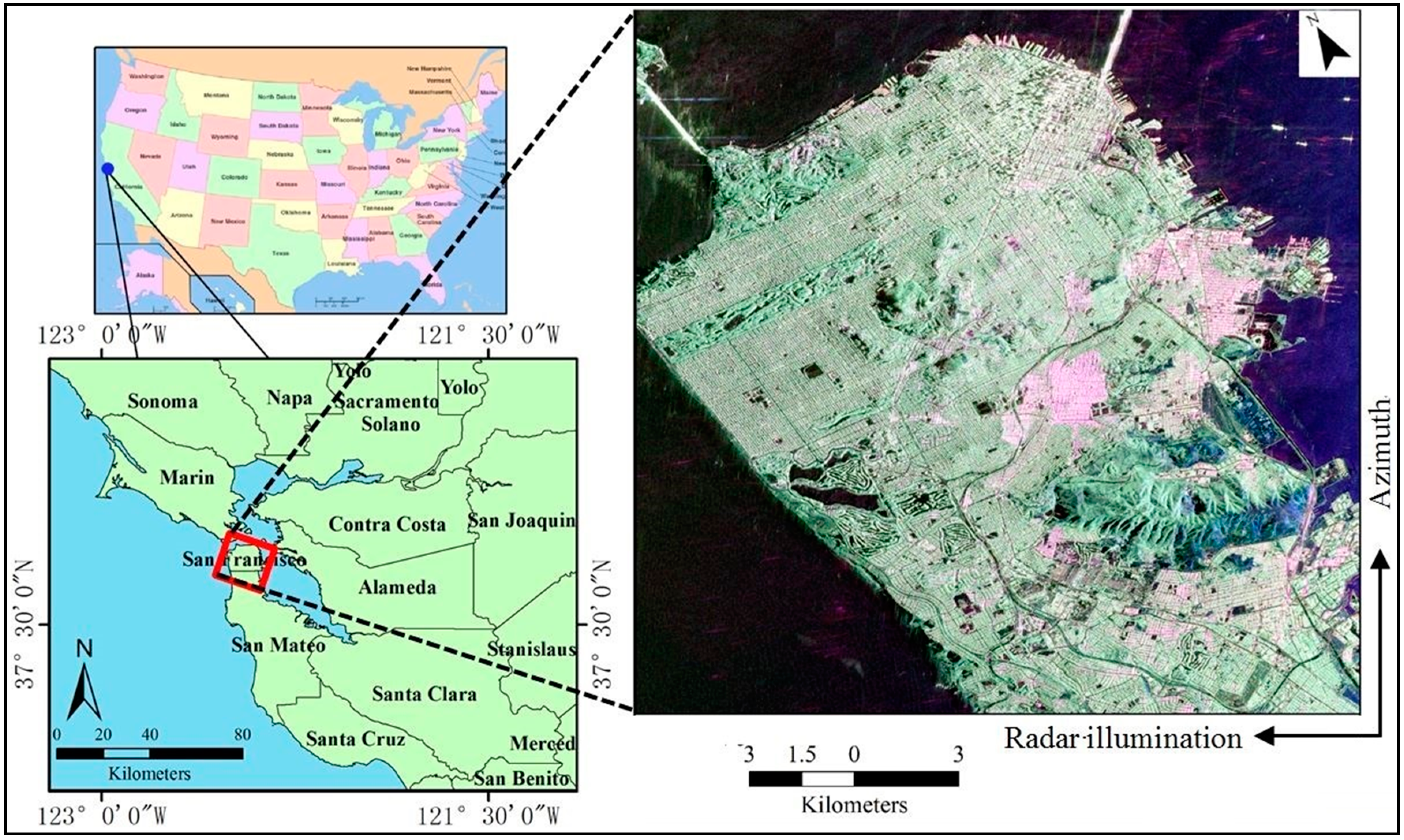
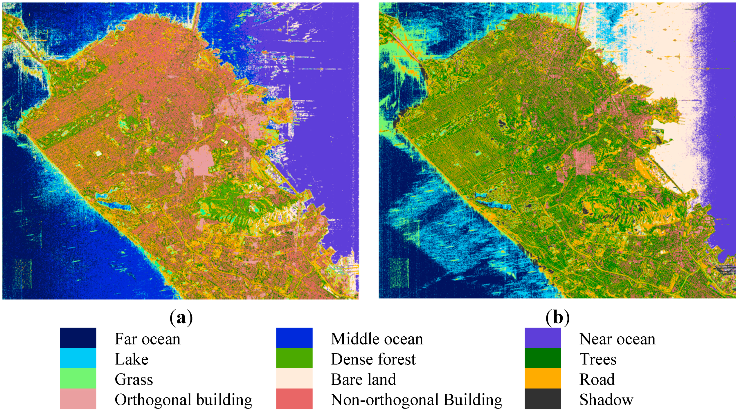
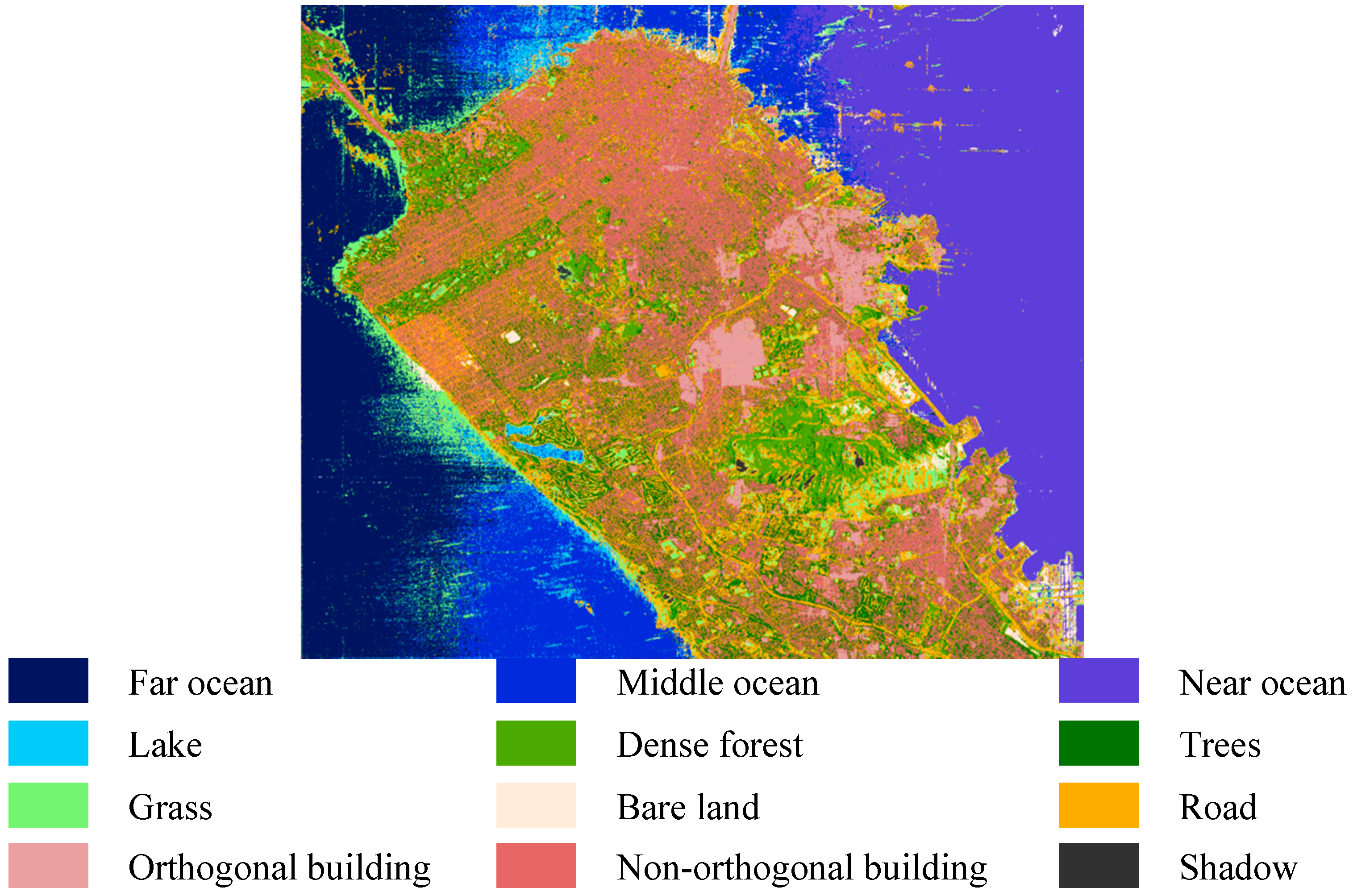
Figure 4a. The study area is a highly urbanized city (San Francisco, CA, USA). Urban structures, including buildings in different orientations and roads are fairly identified. Green covers in urban lands (e.g., parks) are clear. Ocean surfaces also show clear tonal differences from far range to near range.
Figure 4. Classification results of proposed method and Wishart supervised method on L-band data; (a) proposed method; (b) Wishart supervised method.
Remotesensing 07 04157 g004
As a comparison, the commonly applied Wishart supervised classification [11] was also performed with the L-band image. The Wishart supervised classification (Figure 4b) is more greenish than that of the proposed method, revealing apparent overestimation of green covers. Correspondingly, urban structures are severely underestimated. The near ocean is misclassified as bare land (pink area in the upper right), while the far ocean is confused with lake and near ocean in the left and grass near the bridge in the upper left corner. Between Figure 4a,b, our proposed method yields the overall distributions of land surfaces that are similar to the original image.
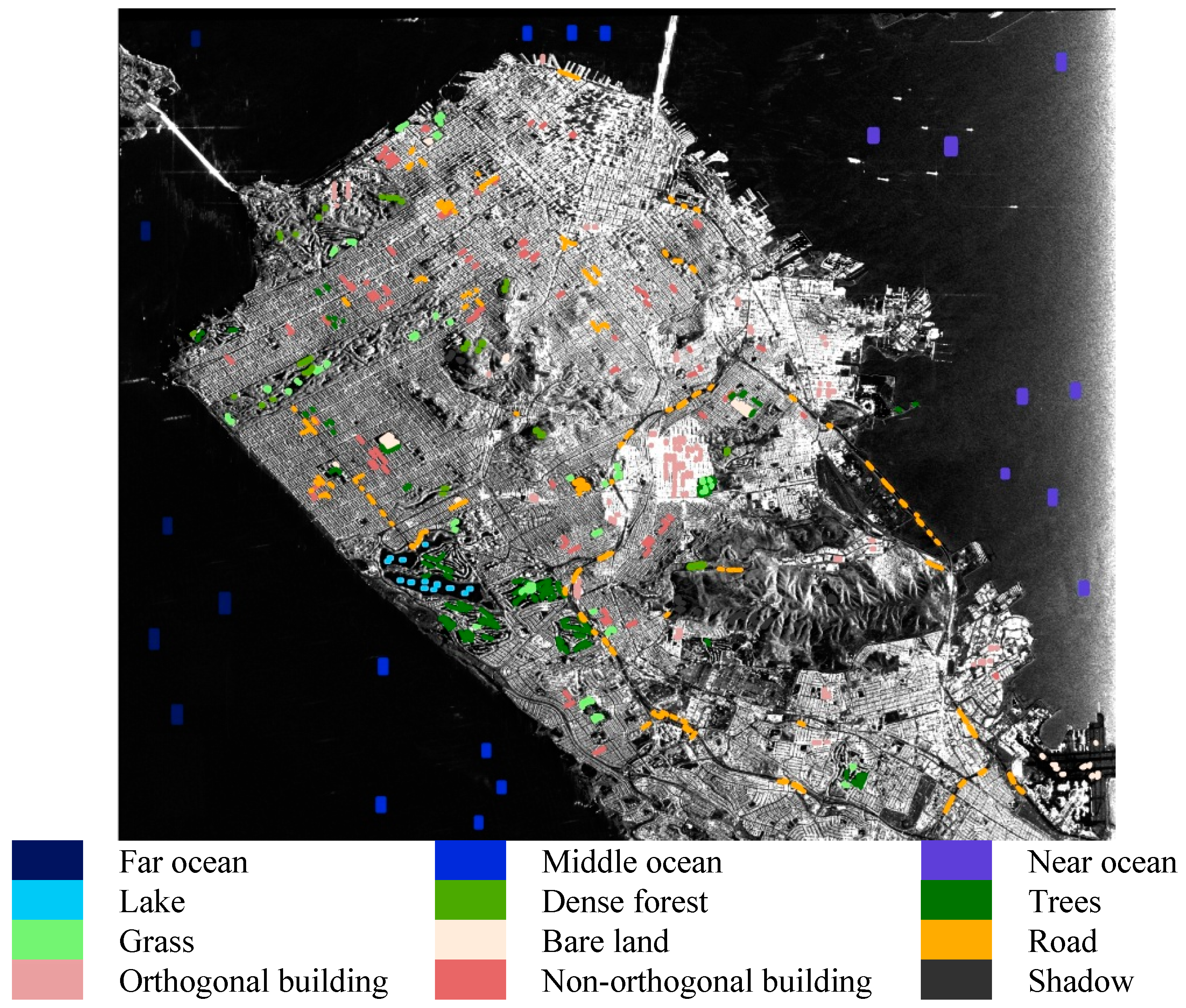
Using the validation points in Table 1, the accuracies the two classifications in Figure 4 are also compared with a confusion matrix approach (Table 4 and Table 5).
Table 4. Confusion Matrix of the Proposed Method (L-band).
Classified DataReference Data
BLOBNBFODFTSLKMONOGSRDSDUA (%)
BL75800000400644191.22
OB012901100900003098.25
NB0101408015225000052082.34
FO0002150005710110096.11
DF0019083847000313590.59
TS02124022785000033081.26
LK10040020910031091.67
MO0005000411867100095.30
NO50000000210500099.76
GS90000109001340992485.73
RD35022086200011913433882.54
SD400000300211656492.76
PA (%)84.8899.0888.8997.5594.869.5977.1295.8499.9585.8485.8789.24-
OA (%): 91.17; kappa: 0.90.
Table 5. Confusion Matrix of the Wishart Supervised Classification (L-band).
Classified DataReference Data
BLOBNBFODFTSLKMONOGSRDSDUA (%)
BL110000001481012601.29
OB07203900100000094.74
NB05526640036500002041.95
FO00016200023944090062.40
DF1421505542030001180047.84
TS0266600253509000017034.74
LK000537001819822170010.53
MO000000000000N/A
NO850000000129400093.84
GS3950047013880648402242.05
RD24306077480002935797143.96
SD15800001290058137855932.77
PA (%)1.2355.3041.9273.5062.6745.1266.790.0061.4441.5137.0288.45-
OA (%): 45.65; kappa: 0.41.
The overall accuracy (OA) of the proposed method was 91.17%, much higher than that of Wishart supervised classification (45.65%). The kappa value of the proposed method was 0.90, also much higher than 0.41 of the Wishart supervised classification. Furthermore, the producer’s (PA) and user’s (UA) accuracies were higher than those of the Wishart supervised classification for all classes. As an example, the UA and PA of bare land (BL) evaluated by the Wishart supervised classifier was 1.29% and 1.23%, respectively. As indicated by the confusion matrix, bare land was frequently confused with near ocean, grass and road. The proposed method greatly alleviated this situation, improving the UA and PA to 91.22% and 84.88%, respectively. For the example of non-orthogonal buildings (NB), the Wishart supervised classifier dramatically confused it with dense forest (DF) and trees (TS), yielding the UA and PA of 41.95% and 41.92%, respectively. The proposed method largely remedied the confusion and increased the UA and PA to 82.34% and 88.89%. Similar results were obtained for classifications with C- and P-band data. The results indicate a huge improvement of classification with the proposed method in urban lands.

4.2. Contribution of Polarimetric and TF Features

The contribution was assessed by performing the C5.0 decision tree classification using a specific type of features (polarimetric or TF) each time. Their overall accuracies and Kappa values are compared with the all-feature classification that we proposed in this study (Table 6).
Classification with full features reached the highest accuracies. By using polarimetric features (POL-only) in the classification, the overall accuracy for each band was about 3%–5% lower than the full-feature classification. The kappa coefficients were also decreased. Using TF information itself (TF-only), the overall accuracies were dramatically reduced, with approximately 14% in the C-band, 13% in the L-band and 17% in the P-band. The kappa coefficients also significantly decreased. Therefore, polarimetric features played a better role in POLSAR image classification than TF features.
Table 6. Accuracies for classification with full features (proposed), polarimetric features (POL-only) and TF features (TF-only) of the three images.
C-Band L-BandP-Band
OA (%)KappaOA (%)KappaOA (%)Kappa
Proposed90.450.8991.170.9084.910.83
POL-only84.740.8388.290.8780.850.79
TF-only76.490.7478.300.7667.640.64
In order to investigate the contribution of TF and polarimetric features to the accuracies of different classes, their producer’s (PA) and user’s (UA) accuracies with L-band image are listed in Table 7.
In comparison with our classification using full features, the PAs and UAs of different ground objects decreased when POL- or TF-only information was used. It indicates that both TF and polarimetric information are important in the proposed method. The POL-only method significantly reduced the PA and UA of DF (dense forest), TS (trees) and LK (lakes) (>5%), indicating that TF information is required for accurately classifying these ground objects. The TF-only method also considerably decreased the PA and UA of ground objects. The decline in PA and UA of bare land and lake exceeded 20%. Therefore, polarimetric information is important for accurately classifying bare land, lake and central ocean areas.
Table 7. PA and UA of POL-only and TF-only method on L-band.
PA (%)UA (%)
ProposedPOL-OnlyTF-OnlyProposedPOL-OnlyTF-Only
bare land (BL)84.8885.8948.4991.2289.6068.62
orthogonal building (OB)99.0899.0894.3998.2597.9590.30
non-orthogonal building (NB)88.8984.9176.3982.3477.0372.80
far Ocean (OFOF)97.5595.5589.0796.1193.8983.32
dense forest (DF)94.8087.2291.2990.5977.4179.82
trees (TS)69.5957.5459.4981.2673.0971.23
lake (LK)77.1259.0454.6191.6784.2166.37
middle ocean (MO)95.8495.2377.4195.3093.7879.45
near ocean (NO)99.9599.9599.5399.7699.9196.90
grass (GS)85.8485.1467.0185.7384.1760.05
road (RD)85.8780.9564.5882.5479.9766.71
shadow (SD)89.2487.1874.0592.7692.7681.53
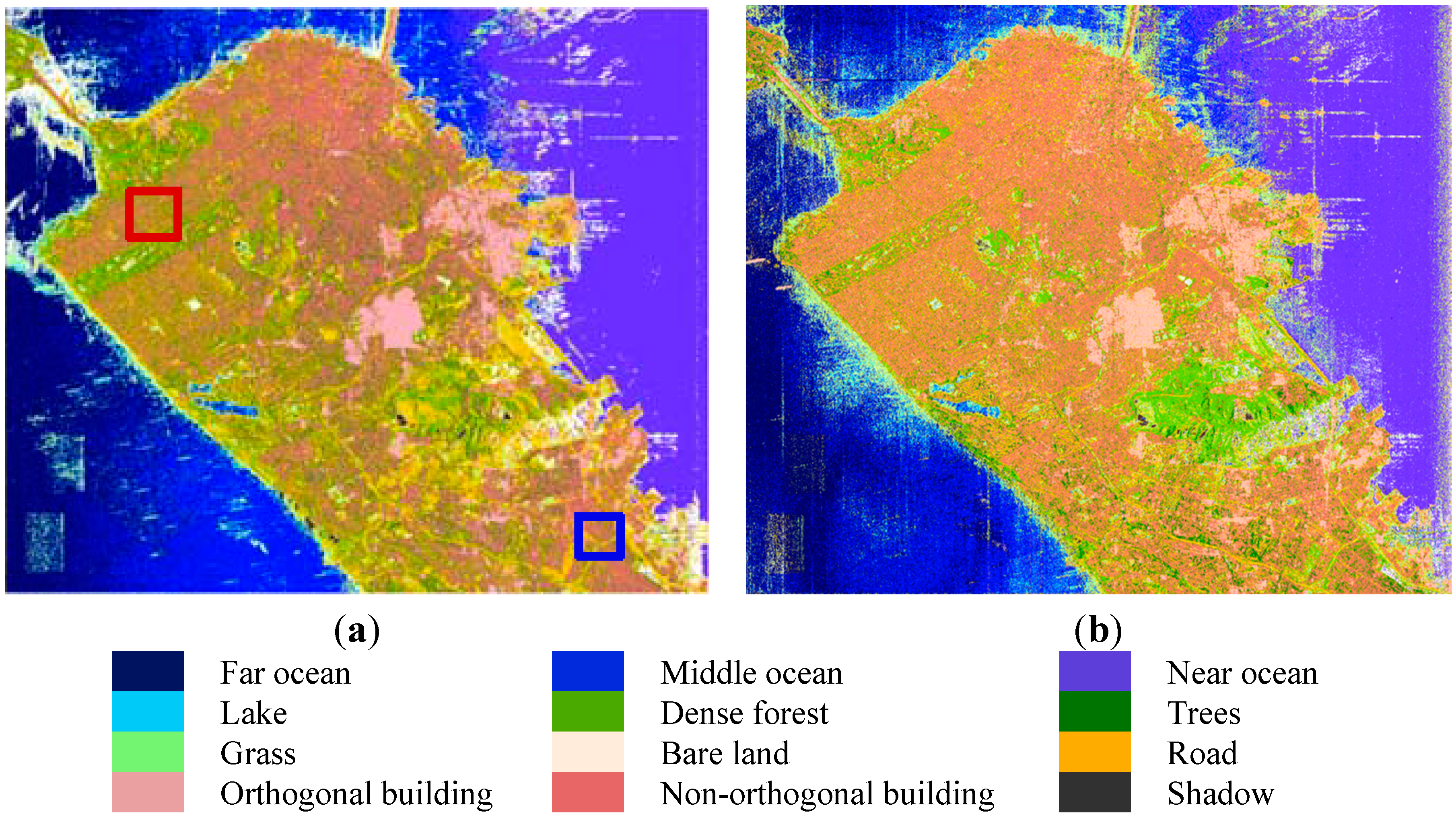
Figure 5 shows the results of POL-only and TF-only classifications on L-band data. In the absence of TF information (Figure 5a), higher misclassifications were observed than the proposed full-feature classification in Figure 4a. For example, near the bridge in the upper left corner, the far ocean was misclassified as bare land. In the absence of polarimetric information (Figure 5b), some green areas in urban lands were misclassified as buildings. Two subsets of the image (marked as the red and blue squares in Figure 5) were selected to show more details about the effects of polarimetric and TF information. In these subsets, the original image and the three classification results are visually compared (Figure 6).
Figure 5. Classification results of POL-only and TF-only on L-band data. (a) POL-only; (b) TF-only.
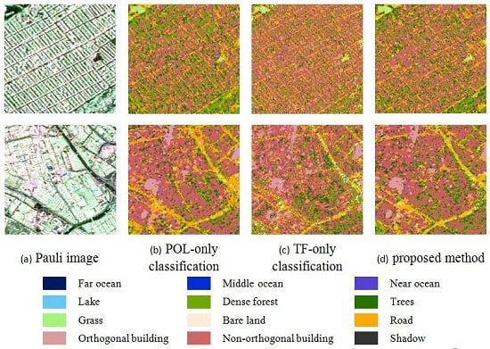
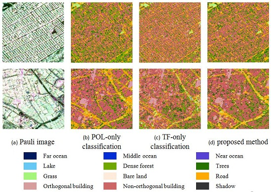
Remotesensing 07 04157 g005
Figure 6. Comparison of classification results in two subsets marked in Figure 5a. (a
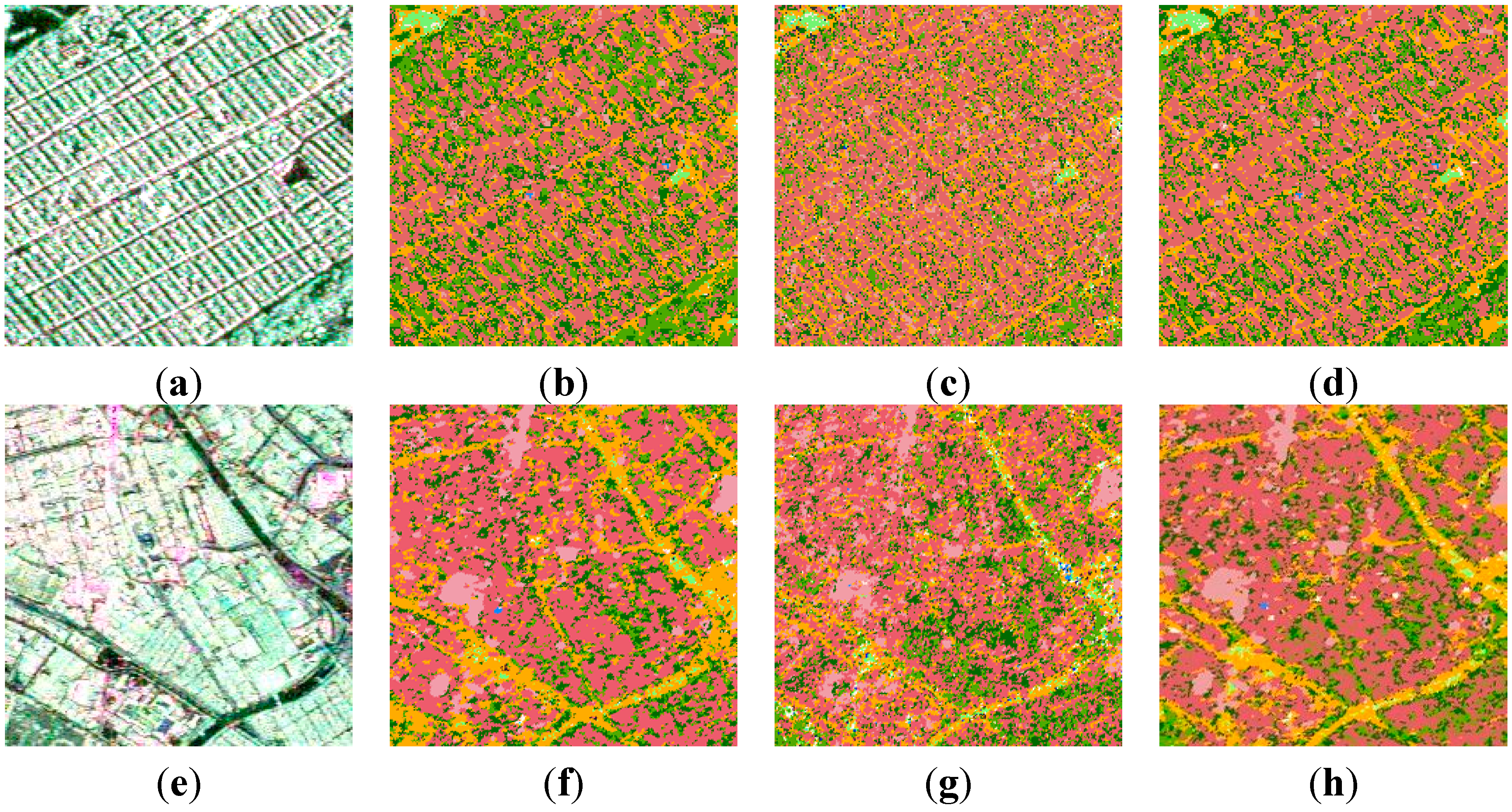
d) represent the red-squired subset: (a) Pauli image (b) POL-only classification (c) TF-only classification (d) proposed method; Figures (eh) represent the blue-squared subset: (e) Pauli image (f) POL-only classification (g) TF-only classification (h) proposed method.
Remotesensing 07 04157 g006
As displayed in Figure 6a, the red-squared subset is a typical dense residential area with regularly oriented dense buildings. Compared with the full-feature classification (Figure 6d), removing TF information (Figure 6b) resulted in misclassifying buildings to dense forest. The importance of TF information in delineating dense forest from non-orthogonal buildings has also been reported in previous studies [42]. On Google Earth, the blue-squared subset is a newly developed commercial and light industrial land. It has mixed cover of buildings, parking lots and open spaces with dense road networks (e.g., highways) (Figure 6e). For road classification, the TF-only classification results in coarse clusters (Figure 6g), while the POL-only classification (Figure 6f) is noisy. It is the combination of TF and polarimetric features that contributes to a reasonable classification result in Figure 6h. This phenomenon is in conformity with the analysis of accuracy of road classification in Table 7.

4.3. Contribution of C5.0 Decision Tree Algorithm

To evaluate the contribution of the C5.0 decision tree algorithm in the proposed method, the algorithm was replaced by various alternative classifiers [19] in L-band; neural network (NN), and SVMs with different kernel functions-radial basis function (SVM-RBF) and polynomial (SVM-POLY) [19]. The OA and kappa values of the classification results are listed in Table 8.
From the table, the highest accuracies and kappa coefficients in each band were obtained by the proposed method. This indicates that the C5.0 decision tree classifier adopted in the proposed method is more effective than the other tested classifiers. Moreover, the Wishart supervised classifier yielded the lowest classification accuracy, while the classifier with multiple features achieved a relatively high accuracy, revealing that accurate classification requires the integration of multiple features. Finally, regardless of classifier, P-band data were classified with the lowest accuracy. This behavior may be caused by the long wavelength of the P-band. Ground features in most urban areas are difficult to distinguish due to the complex scattering mechanisms of signals at longer wavelengths.
Table 8. Classification Accuracy of Different Classifiers.
OA (%)Kappa
Proposed91.170.90
Quest71.850.69
NN86.000.84
SVM-RBF88.810.88
SVM-POLY88.410.87
Wishart45.650.41
QUEST decision tree is designed to reduce the processing time required for the large decision tree analysis. Compared with QUEST, the rule of C5.0 decision tree is more complex, but it allows for more than two subgroups of segmentation many times. SVM is computationally expensive. Neural network has a strong ability of nonlinear fitting, but it is difficult to provide clear classification rules. C5.0 decision tree has a better performance on feature space optimization and feature selection, especially when the feature set is large [24].

4.4. Contribution of Multi-Frequency Dataset

Radar signals at different wavelengths exhibit different sensitivities to ground features [43,44]. Thus, combining multiple bands might be helpful for ground imaging. Here, POLSAR data of three frequencies are combined and input to C5.0 decision tree. The results of this test are shown in Figure 7 and Table 9.
Figure 7. Classification results of adding C- and P-band data to L-band data.
Remotesensing 07 04157 g007
Compared with other results, simultaneous use of C-, L- and P-band data further reduces the quantities of confused pixels between classes. For example, misclassification is diminished near the bridge in Figure 7, and the distribution of vegetation and buildings is more comparable to the high-resolution image at Google Earth.
Table 9. Accuracy of Multi-Frequency Dataset.
Band SelectionOA (%)Kappa
C90.450.89
L91.170.90
P84.910.83
C+L95.560.95
C+P94.780.94
L+P94.890.94
C+L+P96.390.96
In Table 9, combining any two bands dramatically increased the accuracies compared to any single-frequency classification. Using all of C-, L, and P-band data reached the highest OA (96.39%) and Kappa coefficient (0.96). In order to study the effects of single bands and band combinations of classification accuracy on different ground objects more clearly, PA and UA of typical classes were provided in
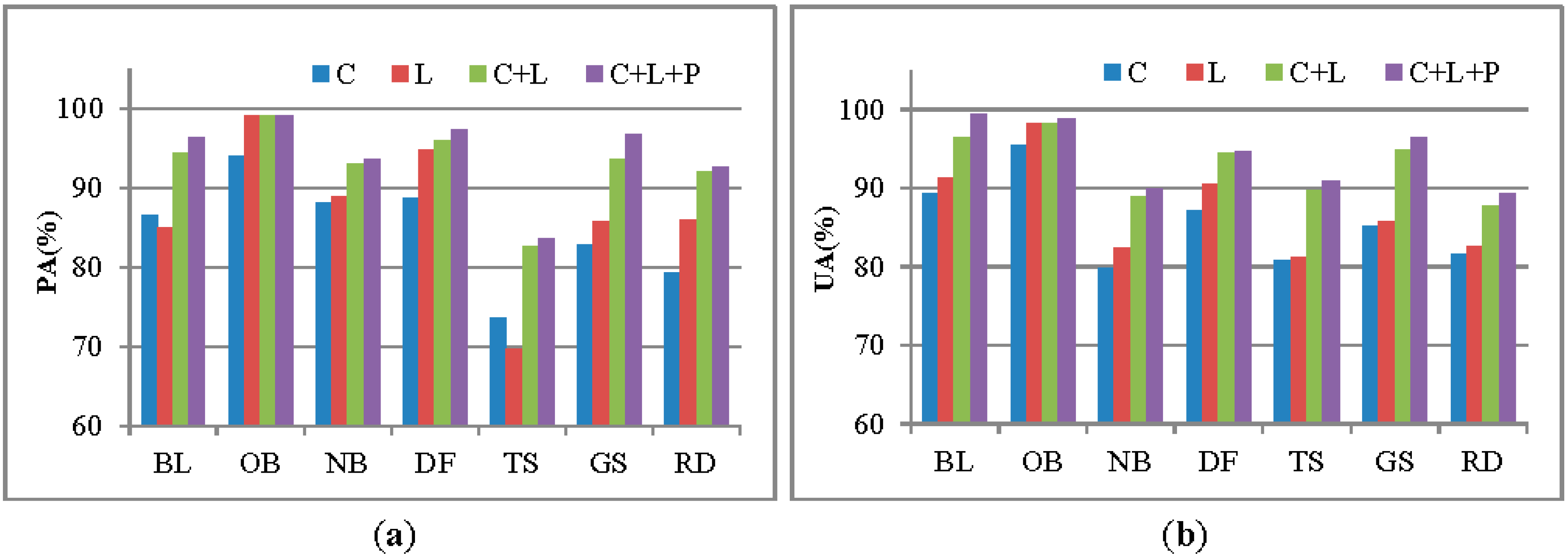
 Figure 8.
Figure 8. PA and UA histogram of Multi-Frequency Dataset.
Remotesensing 07 04157 g008
From the Figure 8a, PA of trees in C-band was higher than that in L-band, while PA of orthogonal building in C-band was lower. Comparing the scattering mechanisms at different frequencies, the C-band return is primarily from volume scattering in the vegetation canopy, whereas L-band scattering is stronger for ground as well as double bounce in urban areas. The L-band classification plays better in the distinction among forest, trees, and building. At higher frequencies, POLSAR data are less sensitive to azimuth slope variations because electromagnetic waves at short wavelength are more sensitive and less penetrative to small scatterers. This may explain the poorest performance of P-band classification.
Classification accuracies of multi-frequency dataset performed better than those of single bands. For instance, using the combination of C- and L-band datasets, the PA of each class was increased, compared with that of a single band. The PA and UA of trees, grass, and non-orthogonal buildings were enhanced to a large degree. As waves at different wavelength are sensitive to various scatterers, the methods using the combination among different bands dataset for comprehensive utilization of this nature makes the classification precision improvement. Overall, the C- and L-band PolSAR data are more suitable for single band data classification, and multi-band classification performs much better than any single-band data.

4.5. Stable Features in POLSAR Image Classification

When all POLSAR features are included, the proposed method reaches high classification accuracy. However, practically, it is time consuming and inefficient to collect such a large set of features from POLSAR imagery. With reduced sets of features, the complexity of the C5.0 decision tree can be effectively decreased and the applicability improved. For this purpose, all features (100%) involved in the proposed method were sorted by their predictor importance (calculated by the C5.0 decision tree algorithm) to test the feasibility of feature reduction. The feature groups at top-ranking 50%, 40%, 30%, 20% and 10% were selected and classified in the C5.0 approach. The accuracies are compared in Table 10.
Table 10. Overall Accuracies of classification with reduced features.
C-BandL-BandP-Band
100%90.45%91.17%84.91%
50%90.10%91.00%84.42%
40%89.79%90.66%84.95%
30%89.39%90.17%84.72%
20%85.59%88.55%84.78%
10%79.64%85.65%81.87%
For all images in three frequencies, the overall accuracies were similar when using 100%, top 50%, 40%, and 30% features. Accuracies slightly changed when features used in classifications dropped to 20%. When only 10% of features were used, however, there was a relatively large decrease of the accuracies. Therefore, the top-ranking 20% of features are a reasonable set of input features for classification. Table 11 lists the top 20% of features used in the proposed method of C-, L- and P-band in a descending order of their predictor importance scores. For images at different frequencies, a different set of features was included in each rank. Four features were always selected: three polarimetric features including H/A/Alpha decomposition (entropy), Shannon entropy, and T11 Coherency Matrix element that describes the single scattering flat surface (or odd scattering), and one TF feature that is the intensity of coherence of HH. These four features are highlighted in bold in Table 11.
Using these four features as inputs, the accuracies of the proposed method and the Wishart supervised classification method are compared in Table 12.
For all frequencies, the overall accuracies of the proposed methods were around 30% higher than the Wishart supervised method. For the C-band image, its accuracy was even higher than the top 10% features as listed in Table 10. Interestingly, with only four features, classification of the C-band image reached the highest accuracy, while that of the L-band image had the best results when more features were used (as shown in Table 10). The P-band image turned out to have the lowest accuracies for all combination of features, which could be related to noises introduced by more complex interaction between longer wavelength signals and heterogeneous urban surfaces.
Table 11. Top 20% of features in the proposed method of C-, L- and P-band.
C-BandL-BandP-Band
Shannon EntropyVanZyl_VolShannon Entropy
(TF)Δalpha(TF)intensity of coherence of HH(TF)intensity of coherence of HH
(TF)intensity of coherence of HHShannon EntropyNeum2_Pha
T11Yam3_VolEntropy
ConformityCoefficientSERDKrog_H
Krog_DFreeman_Vol(TF) Intensity interferogram of HH
Yam3_VolDepolarization indexDERD
PedestalHeightYam4_VolHolm2_T22
(TF)Intensity interferogram of HHYam4_DblHuynen_T22
Yam3_DblCloude_T33Anisotropy
Yam3_OddFreeman2_VolT11
EntropyTouzi_tau2Conformity Coefficient
Holm1_T22Freeman_DblBarnes2_T11
Huynen_T22Krog_SHuynen_T33
AnisotropyT11Touzi_tau1
Cloude_T11Touzi_alpha1(TF)ΔYam4_Odd
Touzi_tau1Entropyalpha3
VanZyl_Volalpha2(TF) amplitude coherence of HV
(TF) Intensity interferogram of HVVanZyl_OddYam4_Hlx
The four features in bold are the stable features which exist in the top 20% of features used in the proposed method of C-, L- and P-band. (TF) stands for TF feature, others are polarimetric features.
Table 12. Overall Accuracy of Wishart supervised method and proposed method using only 4 features.
C-BandL-BandP-Band
Wishart supervised56.44%45.65%43.20%
Proposed method82.22%79.38%73.20%

5. Discussion

The proposed method mines the information inherent in POLSAR images, and achieves relatively high classification accuracies without support from other data. For example, repeat-pass interferometry improves the classification of ground features, such as buildings [40]. However, a polarimetric interference dataset is difficult to obtain, and incurs high cost. In the absence of a repeat-pass interferometric dataset, the proposed method obtains interferometric information between different sub-aperture images using the TF technique.
The benefit of the proposed method is revealed in several ways. First, the data are processed images without the need of complex pre-processes as needed for raw data. Second, the model adopts the well-established TF and polarization decomposition techniques and the C5.0 decision tree algorithm, which can be easily implemented and integrated. Third, the proposed method is compatible with different POLSAR features and classifiers. Accordingly, our procedure is adaptable to new features or classifiers. For example, the QUEST algorithm [45] is less accurate than the C5.0 algorithm, but its tree depth can be controlled to decrease the complexity of the classification rules. Hence, the C5.0 could be replaced by this algorithm if a simple decision tree is sufficient. Finally, the classical Wishart supervised classification assumes a Gaussian distribution of ground features. This assumption is suitable for natural environments with relatively homogeneous land covers, but not viable in urban areas. Therefore, the Wishart supervised classification yields low accuracy in the present study. In contrast, the proposed method is decision tree-based and does not require a hypothesized statistical distribution, and is applicable to various land covers. Different from black box algorithms, such as neural networks, the proposed method is a white box. The given classification rule in each branch reveals the ground objects associated with specific POLSAR features. Therefore, the proposed method can yield a clear physical explanation.
Among the rich set of POLSAR features, three polarimetric features (H/A/Alpha entropy, Shannon entropy, T11) and one TF feature (HH coherence intensity) are found always holding high importance in urban classification of the test site. T11 stands for single or odd-bounce scattering, entropy measures the degree of the randomness of the scattering process, for which entropy→0 corresponds to a pure target, whereas entropy→1 means the target is a distributed one. Shannon entropy [46] is a way of quantifying the disorder of random variables, it is the sum of two contributions related to intensity and polarimetry of PolSAR data. So it can determine which fraction of the disorder quantified by the entropy comes from intensity fluctuations from depolarization, and from incoherence. The fluctuating random variables have high value of Shannon entropy, while the quasi-deterministic random variables have relatively low value. Intensity of coherence of HH is the coherence generated by PolInSAR technique using the two sub-aperture images from the full-resolution POLSAR data. These features played different roles in urban classification. For example, TF information (HH coherence intensity) could be very helpful in distinguishing dense forest and slant-buildings. Generally, buildings have the typical characteristics of double-bounce scattering, and dense forest has the typical characteristics of volume scattering. However, some buildings have specific orientations not aligned in the azimuth direction or have complex structures, which may cause significant depolarization and produce high cross-polar levels that can appear as volume scattering. Consequently, those buildings were classified as a volume class, and then misinterpreted as dense forest (Figure 3b). But in the two sub-aperture images, buildings, unlike dense forest, are high-coherence targets, thus TF information can separate buildings from dense forest. The selection of POLSAR features is related to physical properties of ground objects and their distributions. Better understanding of these features is thus important in advancing POLSAR applications.
As demonstrated in this study, accuracies of POLSAR image classification also vary using data acquired in different frequencies. One may notice that C- and L-band data achieve higher accuracies than P-band (Table 8). The possible reason is that the shorter wavelength (C, L) can get more spatial information than the longer (P-band) in high-density urban area. But multi-frequency information has strong mutual complementariness. For example, the long wavelength of P-band supplies electromagnetic scattering information that is unobservable in the C- or L-band, but reveals less detailed spatial information. By combining the P-band data with those of the C- and L-bands, the electromagnetic and spatial details can be fully utilized to enhance the delineation of ground objects. Additionally, some studies have shown that other features, such as the object-oriented spatial information, are also useful in POLSAR image classification [40]. More experiments will be conducted in the future to investigate the contribution of these new features in urban mapping.

6. Conclusions

This study integrates time-frequency information, polarimetric information and C5.0 decision tree into a novel approach to performing POLSAR image classification in an urban area. The integrated results achieved an overall classification accuracy around 90% on C- and L-band data, and 85% on P-band data, much higher than the Wishart supervised classification. Polarimetric information better distinguished among bare land, lake and ocean, while TF information reduced the confusion between urban/built-up areas and vegetation. Four stable features, entropy, Shannon entropy, T11 and HH intensity of coherence, are found more useful than other POLSAR features in urban classification. This approach provides a superior way of classifying urban areas from multi-band POLSAR imagery.

Acknowledgment

This research is supported by National Natural Science Foundation of China, Project No.: 40801172, and Beijing Natural Science Foundation, Project No.: 4142011. The authors would like to thank JPL AIRSAR for providing valuable polarimetric SAR data.

Author Contributions

Lei Deng conducted the study and developed the proposed methodology. Lei Deng and Ya-nan Yan carried out the results validation and analysis, and wrote the manuscript. Cui-zhen Wang and Lei Deng were involved in discussing its results and revising the manuscript.

Conflicts of Interest

The authors declare no conflict of interest.

References

  1. Wang, W.; Lu, F.; Sun, Z.W.; Wang, J. A novel unsupervised classifier of polarimetric SAR images. Procedia Eng. 2011, 15, 1595–1599. [Google Scholar] [CrossRef]
  2. Lee, J.S.; Pottier, E. Polarimetric Radar Imaging: From Basics to Applications; CRC press: Raton, FL, USA, 2009; pp. 235–350. [Google Scholar]
  3. Papoulis, A. Probability, Random Variables, and Stochastic Processes; McGraw-Hill: New York, NY, USA, 1965. [Google Scholar]
  4. Freitas, C.; Soler, L.; Sant’Anna, S.J.S.; Dutra, L.V.; Dos Santos, J.R.; Mura, J.C.; Correia, A.H. Land use and land cover mapping in the brazilian amazon using polarimetric airborne P-band SAR data. IEEE Trans. Geosci. Remote Sens. 2008, 46, 2956–2970. [Google Scholar] [CrossRef]
  5. Formont, P.; Pascal, F.; Vasile, G.; Ovarlez, J.; Ferro-Famil, L. Statistical classification for heterogeneous polarimetric SAR images. IEEE J. Sel. Top. Signal Proc. 2011, 5, 567–576. [Google Scholar] [CrossRef]
  6. Ince, T. Unsupervised classification of polarimetric SAR image with dynamic clustering: An image processing approach. Adv. Eng. Softw. 2010, 41, 636–646. [Google Scholar] [CrossRef]
  7. Kersten, P.R.; Lee, J.S.; Ainsworth, T.L. Unsupervised classification of polarimetric synthetic aperture radar images using fuzzy clustering and EM clustering. IEEE Trans. Geosci. Remote Sens. 2005, 43, 519–527. [Google Scholar] [CrossRef]
  8. Cloude, S.R.; Pottier, E. An entropy based classification scheme for land applications of polarimetric SAR. IEEE Trans. Geosci. Remote Sens. 1997, 35, 68–78. [Google Scholar] [CrossRef]
  9. Freeman, A.; Durden, S.L. A three-component scattering model for polarimetric SAR data. IEEE Trans. Geosci. Remote Sens. 1998, 36, 963–973. [Google Scholar] [CrossRef]
  10. Yamaguchi, Y.; Yajima, Y.; Yamada, H. A four-component decomposition of POLSAR images based on the coherency matrix. IEEE Geosci. Remote Sens. Lett. 2006, 3, 292–296. [Google Scholar] [CrossRef]
  11. Kong, J.A.; Swartz, A.A.; Yueh, H.A.; Novak, L.M.; Shin, R.T. Identification of terrain cover using the optimum polarimetric classifier. J. Electromagn. Waves Appl. 1988, 2, 171–194. [Google Scholar]
  12. Lee, J.S.; Grunes, M.R.; Kwok, R. Classification of multi-look polarimetric SAR imagery based on complex wishart distribution. Int. J. Remote Sens. 1994, 15, 2299–2311. [Google Scholar] [CrossRef]
  13. Lee, J.S.; Grunes, M.R.; Ainsworth, T.L.; Du, L.J.; Schuler, D.L.; Cloude, S.R. Unsupervised classification using polarimetric decomposition and the complex Wishart classifier. IEEE Trans. Geosci. Remote Sens. 1999, 37, 2249–2258. [Google Scholar] [CrossRef]
  14. Shimoni, M.; Borghys, D.; Heremans, R.; Perneel, C.; Acheroy, M. Fusion of PolSAR and PolInSAR data for land cover classification. Int. J. Appl. Earth Obs. Geoinf. 2009, 11, 169–180. [Google Scholar] [CrossRef]
  15. Lee, J.S.; Grunes, M.R.; Pottier, E. Quantitative comparison of classification capability: Fully polarimetric versus dual and single-polarization SAR. IEEE Trans. Geosci. Remote Sens. 2001, 39, 2343–2351. [Google Scholar] [CrossRef]
  16. Fukuda, S.; Hirosawa, H. A wavelet-based texture feature set applied to classification of multifrequency polarimetric SAR images. IEEE Trans. Geosci. Remote Sens. 1999, 37, 2282–2286. [Google Scholar] [CrossRef]
  17. Arzandeh, S.; Wang, J. Texture evaluation of RADARSAT imagery for wetland mapping. Can. J. Remote Sens. 2002, 28, 653–666. [Google Scholar] [CrossRef]
  18. Dixon, W.J.; Massey, F.J. Introduction to Statistical Analysis; McGraw-Hill: New York, NY, USA, 1969. [Google Scholar]
  19. Bishop, C.M. Pattern Recognition and Machine Learning; Springer: New York, NY, USA, 2006. [Google Scholar]
  20. Pajares, G.; López-Martínez, C.; Sánchez-Lladó, F.J.; Molina, Í. Improving Wishart classification of polarimetric SAR data using the Hopfield Neural Network optimization approach. Remote Sens. 2012, 4, 3571–3595. [Google Scholar]
  21. Rowley, H.A.; Baluja, S.; Kanade, T. Neural network-based face detection. IEEE Trans. Pattern Anal. Mach. Intell. 1998, 20, 23–38. [Google Scholar] [CrossRef]
  22. Sánchez-Lladó, F.J.; Pajares, G.; López-Martínez, C. Improving the Wishart synthetic aperture radar image classifications through deterministic simulated annealing. ISPRS J. Photogramm. Remote Sens. 2011, 66, 845–857. [Google Scholar] [CrossRef]
  23. Ferro-Famil, L.; Reigber, A.; Pottier, E. Nonstationary natural media analysis from polarimetric SAR data using a two-dimensional time-frequency decomposition approach. Can. J. Remote Sens. 2005, 31, 21–29. [Google Scholar] [CrossRef]
  24. Pang, S.L.; Gong, J.Z. C5.0 classification algorithm and application on individual credit evaluation of banks. Syst. Eng. Theory Pract. 2009, 29, 94–104. [Google Scholar] [CrossRef]
  25. AIRSAR JPL/NASA. Available online: //airsar.jpl.nasa.gov (accessed on 25 January 2013).
  26. Wang, Y.Y.; Li, J. Feature-selection ability of the decision-tree algorithm and the impact of feature-selection/extraction on decision-tree results based on hyperspectral data. Int. J. Remote Sens. 2008, 29, 2993–3010. [Google Scholar] [CrossRef]
  27. Truong-Loi, M.L.; Dubois-Fernandez, P.; Freeman, A.; Pottier, E. The conformity coefficient or how to explore the scattering behaviour from compact polarimetry mode. In Proceedings of the IEEE Radar Conference, Pasadena, CA, USA, 4–8 May 2009; pp. 1–6.
  28. Pampaloni, P.; Paloscia, S. Microwave Radiometry and Remote Sensing of the Earth’s Surface and Atmosphere; ShopeinHK: Hong Kong, China, 2000; pp. 112–143. [Google Scholar]
  29. Zhou, S.H.; Liu, H.; Zhao, Y.; Hu, L. Target spatial and frequency scattering diversity property for diversity MIMO radar. Signal Proc. 2011, 91, 269–276. [Google Scholar] [CrossRef]
  30. Gil, J.J. Polarimetric characterization of light and media. Eur. Phys. J. Appl. Phys. 2007, 40, 1–47. [Google Scholar] [CrossRef]
  31. Nafie, L.A. Vibrational Optical Activity: Principles and Applications; John Wiley & Sons: Hoboken, NJ, USA, 2011; pp. 222–286. [Google Scholar]
  32. Ferro-Famil, L.; Reigber, A.; Pottier, E.; Boerner, W.M. Scene characterization using subaperture polarimetric SAR data. IEEE Trans. Geosci. Remote Sens. 2003, 41, 2264–2276. [Google Scholar] [CrossRef]
  33. Cloude, S.R.; Pottier, E. A review of target decomposition theorems in radar polarimetry. IEEE Trans. Geosci. Remote Sens. 1996, 34, 498–518. [Google Scholar] [CrossRef]
  34. Yamaguchi, Y.; Moriyama, T.; Ishido, M.; Yamada, H. Four-component scattering model for polarimetric SAR image decomposition. IEEE Trans. Geosci. Remote Sens. 2005, 43, 1699–1706. [Google Scholar] [CrossRef]
  35. Schneider, R.Z.; Schneider, R.Z.; Papathanassiou, K.P.; Hajnsek, I.; Moreira, A. Polarimetric and interferometric characterization of coherent scatterers in urban areas. IEEE Trans. Geosci. Remote Sens. 2006, 44, 971–984. [Google Scholar] [CrossRef]
  36. Cloude, S.R.; Papathanassiou, K.P. Polarimetric SAR interferometry. IEEE Trans. Geosci. Remote Sens. 1998, 36, 1551–1565. [Google Scholar] [CrossRef]
  37. Chen, S.W.; Wang, X.S.; Sato, M. PolInSAR complex coherence estimation based on covariance matrix similarity test. IEEE Trans. Geosci. Remote Sens. 2012, 50, 4699–4710. [Google Scholar] [CrossRef]
  38. Reigber, A.; Hellwich, O. RAT (Radar Tools): A Free SAR Image Analysis Software Package. Available online: https://www.cv.tu-berlin.de/fileadmin/fg140/RAT__Radar_Tools_.pdf (accessed on 29 December 2014).
  39. McIver, D.K.; Friedl, M.A. Using prior probabilities in decision-tree classification of remotely sensed data. Remote Sens. Environ. 2002, 81, 253–261. [Google Scholar] [CrossRef]
  40. Qi, Z.; Yeh, A.G.O.; Li, X.; Lin, Z. A novel algorithm for land use and land cover classification using RADARSAT-2 polarimetric SAR data. Remote Sens. Environ. 2012, 118, 21–39. [Google Scholar] [CrossRef]
  41. Quinlan, J.R. Induction of decision trees. Mach. Learn. 1986, 1, 81–106. [Google Scholar]
  42. Deng, L.; Wang, C. Improved building extraction with integrated decomposition of time-frequency and entropy-alpha using polarimetric SAR data. IEEE J. Sel. Top. Appl. Earth Obs. Remote Sens. 2013, 7, 4058–4068. [Google Scholar] [CrossRef]
  43. Frery, A.; Correia, A.H.; Freitas, C.C. Multifrequency full polarimetric SAR classification with multiple sources of statistical evidence. In Proceedings of the IEEE International Conference on Geoscience and Remote Sensing Symposium, Denver, CO, USA, 31 July–4 August 2006; pp. 4195–4197.
  44. Kouskoulas, Y.; Ulaby, F.T.; Pierce, L.E. The Bayesian Hierarchical Classifier (BHC) and its application to short vegetation using multifrequency polarimetric SAR. IEEE Trans. Geosci. Remote Sens. 2004, 42, 469–477. [Google Scholar] [CrossRef]
  45. Loh, W.Y.; Shih, Y.S. Split selection methods for classification trees. Stat. Sin. 1997, 7, 815–840. [Google Scholar]
  46. Réfrégier, P.; Morio, J. Shannon entropy of partially polarized and partially coherent light with Gaussian fluctuations. J. Opt. Soc. Am. A 2006, 23, 3036–3044. [Google Scholar] [CrossRef]

