
Where Aerosols Become Clouds—Potential for Global Analysis Based on CALIPSO Data

Abstract
: This study evaluates the potential to determine the global distribution of hydrated aerosols based on Cloud-Aerosol Lidar and Infrared Pathfinder Satellite Observations (CALIPSO) data products. Knowledge of hydrated aerosol global distribution is of high relevance in the study of the radiative impact of aerosol-cloud interactions on Earth’s climate. The cloud-aerosol discrimination (CAD) score of the Cloud-Aerosol LIdar with Orthogonal Polarization (CALIOP) instrument on the CALIPSO satellite separates aerosols and clouds according to the probability density functions (PDFs) of attenuated backscatter, total color ratio, volume depolarization ratio, altitude and latitude. The pixels that CAD fails to identify as either cloud or aerosol are used here to pinpoint the occurrence of hydrated aerosols and to globally quantify their relative frequency using data of August from 2006 to 2013. Atmospheric features in this no-confidence range mostly match with aerosol PDFs and imply an early hydration state of aerosols. Their strong occurrence during August above the South-East Atlantic and below an altitude of 4 km coincides with the biomass burning season in southern Africa and South America.1. Introduction
Aerosols and clouds are components of a coupled system and mutually affect one another dependent on the meteorological conditions [1,2]. On the one hand, atmospheric aerosols influence cloud properties by altering cloud droplet number concentration, cloud droplet size, cloud albedo and cloud amount. On the other hand, aerosols are influenced by clouds through chemical aging, precipitation scavenging and cloud radiative feedback loops [3–5]. One major challenge in the study of aerosol-cloud interactions (ACI) is to clarify to what extent radiative forcing and precipitation patterns of clouds are a result of cloud feedbacks to aerosols or of meteorological conditions [6,7]. Accordingly, the understanding of ACI and their effect on the Earth’s radiation budget is an important aspect of climate system research.
The complexity of ACI analyses partly stems from the high spatial variability of aerosol properties and cloud dynamics [8–10]. Cloud boundaries are normally blurred by aerosol processing during water uptake, activation as cloud condensation nuclei and growing to cloud droplets (“twilight zone”, [11]). Despite the importance of transition stages between dry aerosols and fully developed clouds, ACI studies commonly use separate aerosol and cloud products distinguished by their optical properties. However, a clear discrimination between clouds and aerosols is not always possible [7,12,13]. Small differences in the probability density functions (PDFs) of cloud and aerosol scattering characteristics have been related to backscatter enhancements due to humidification of aerosols, cloud contamination and remote effects of radiation in the vicinity of clouds [14–17].
The twilight zone with its hydrated aerosols is the region in which ACI mostly occur. Knowing the global distribution and frequency of twilight zones would therefore help understand ACI patterns, pinpoint areas for further research, and ultimately narrow the focus on the processes occurring. The main goal of this study is to explore the usefulness of Cloud-Aerosol LIdar with Orthogonal Polarization (CALIOP) products for identifying regional patterns of hydrated aerosols in the troposphere. Regions where the probability density functions (PDFs) of scattering properties for aerosol and cloud features overlap more often than anywhere else are detected with the help of the CAD score, which is part of Cloud-Aerosol Lidar and Infrared Pathfinder Satellite Observations’ (CALIPSO) Level-2–5 km products [18]. This score classifies pixels as either cloud or aerosol and assigns a confidence level to each. The no-confidence range (NCR) in CAD, i.e., features that are neither classified as cloud nor aerosol with confidence, is the focus of this study. It is assumed that hydrated aerosols fall into this range. With this novel usage of the CAD score and data filters developed for this study, a contribution is made in this paper to the understanding of spatial patterns of processes in aerosol hydration.
The following sections introduce the CAD score, its NCR and the methodology to explore the global occurrence of tropospheric hydrated aerosols. Optical and physical properties are then used to characterize and discuss the NCR features with respect to hydrated aerosols.
2. Data and Methods
The CALIOP instrument on board the CALIPSO satellite is a two-wavelength (532 nm and 1064 nm) polarization ratio-sensitive backscatter lidar and was launched in 2006. It retrieves vertical profiles of aerosol and cloud scattering characteristics along a sun-synchronous satellite orbit track, crossing the equator in the afternoon and repeating every 16 days [13,19,20]. It was chosen for this study as it provides information on cloud and aerosol layer locations and characteristics at the same time [21].
This study uses global CALIPSO Level-2 Layer products of aerosols and clouds (nighttime, Version 3) with a horizontal resolution of 5 km for August 2006 to 2013. This resolution is regarded as appropriate for the study’s focus on global patterns of hydrated aerosols. August data was chosen in this analysis since stratocumulus clouds and aerosols are found off the west coasts of South America and Southern Africa corresponding to increased biomass burning during this month [8,22,23]. Both layer products include spatial and optical information, including layer-averaged attenuated backscatter (AB), layer-integrated attenuated total color ratio (CR), layer-integrated volume depolarization ratio (DR) and CAD score [18]. Only nighttime-data are used, since they have a better detection sensitivity for aerosols and clouds than at daytime due to lower background noise [13,21].
The CAD score is part of CALIOP’s scene classification Level-2 processing algorithm. After a feature is identified as tropospheric according to its altitude relative to the tropopause, the detected object is classified as aerosol or cloud based on the PDFs of five dimensions: AB, CR, DR, altitude, and latitude [13,20,24,25]. The CAD score ranges between −100 and 100. The sign determines the feature type (positive: cloud, negative: aerosol), the absolute value is the confidence level of the classification (high-confidence range: |CAD |≥ 70, no-confidence range (NCR): |CAD |≤ 20). At absolute values smaller than 100, the scattering properties of aerosols and clouds converge, i.e., the PDFs overlap. A CAD score of 0 expresses an equal likelihood of the feature being a cloud and an aerosol, but 0 is also used as a fill value for stratospheric objects [18,20].
By definition the aerosol class consists of all airborne particles, excluding activated water droplets and frozen ice crystals. Accordingly, the cloud class includes any activated water droplets and ice crystals of the high, middle and low cloud families [13].
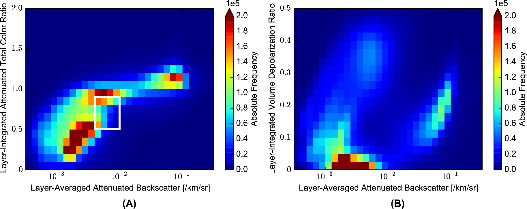
The three dimensions AB, CR and DR of the CAD algorithm help to identify features. AB is defined as the product of the volume backscatter coefficient and the two-way optical transmission from the lidar to the sample volume and can be related to layer thickness. It is corrected for attenuation of the signal by molecules (including ozone). CR is the fraction of the 1064 nm corrected attenuated backscatter coefficients and the corresponding 532 nm corrected attenuated (total) backscatter coefficients. To obtain the DR, the perpendicular is divided by the corresponding parallel channel corrected attenuated backscatter coefficient. CR and DR are integrated between the top and the base of a given layer [26,27].
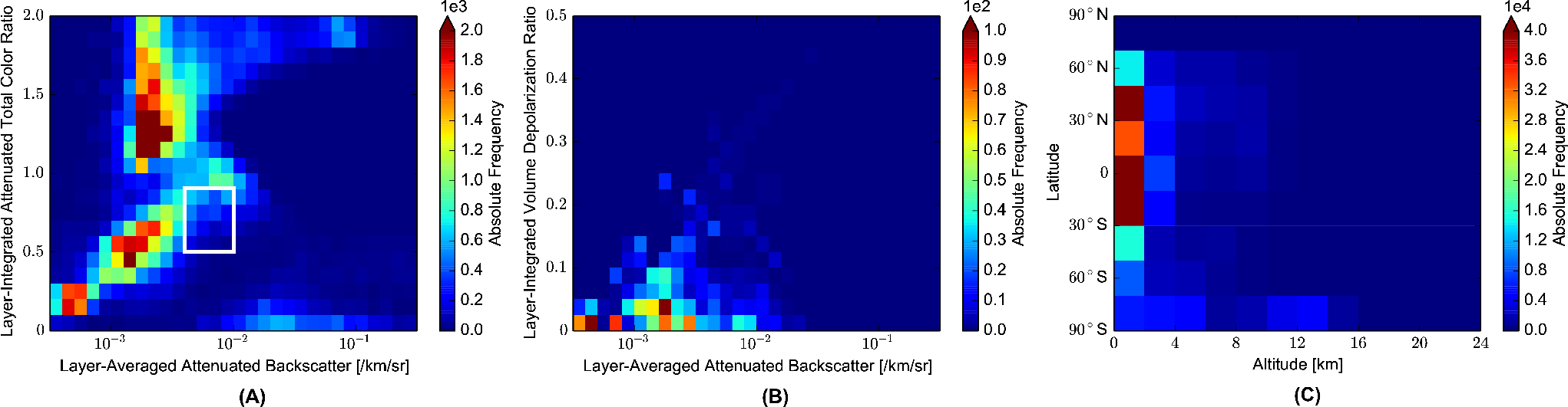
Figure 1 shows the distribution of aerosol (CAD ≤ −70) and cloud (CAD ≥ 70) occurrence frequencies as a function of AB, CR and DR for August from 2006 to 2013. The distribution of aerosol and cloud occurrence frequencies on panel (A) and (B) are in general agreement with e.g., [13,18,20,24,28,29]. In general, aerosols are characterized by a small AB of ∼10−3 km−1 · sr−1 and a CR of ∼0.45, while clouds are bimodally distributed at larger values of AB (∼10−2 and ∼10−1 km−1 · sr−1) and CR (∼0.95 and ∼1.0) [13]. However, this does not hold true for all aerosol and cloud types: desert dust and maritime aerosols in combination with high relative humidities tend to have higher CR values [30]. Dust particles and cirrus clouds because of their non-sphericity and dense water clouds due to multiple scattering have a larger DR than non-dust aerosols [13,18,29]. Typical values for non-dust aerosols, water and ice clouds are summarized in Table 1.
The overlap region between aerosols and clouds (marked in Figure 1) is approximately located by [13,20] between an AB of ∼10−2.4 km−1 · sr−1 and CR of 0.5, and an AB of ∼10−2 km−1 · sr−1 with CR of 0.9 based on CALIOP test data (altitude of 0–1 km and 2–3 km). Apparently, the proposed overlap region fits well into the gap between global aerosol and cloud features found in the troposphere. This may include dense dust and smoke aerosols, thin ice and water clouds, hygroscopic aerosols under humid conditions and mixtures of aerosols and cloud layers [13,14,30]. The CAD algorithm should incorporate parts of the overlap in low CAD scores (NCR) by design, depending on DR, latitude and altitude. The overlap region shifts to smaller values of CR and AB with increasing latitude and altitude [13,20,30]. It may occur that features contained in the overlap of cloud and aerosol PDFs are classified as |CAD |> 20 or that features of NCR could have another reason than presenting the overlap between the cloud and aerosol PDFs [30,31]. In particular, the CAD algorithm is biased towards classifying unknown or partly cloud-contaminated features as cloud [17,21].
According to [20], objects falling in the range between −10 and 20 are partially composed of outliers which are neither cloud nor aerosol layers and located far outside the cloud and aerosol clusters in the PDF space. Most of the features are classified as “unknown cloud“ by convention. These “pseudo-features“ have erroneous scattering characteristics due to signal noise, multiple scattering effects or artificial signal enhancements. The latter is caused by non-ideal detector transient response or an overestimation of the attenuation due to overlying layers [13,31].
Yang [17] showed that the CAD score is strongly related to the backscatter behavior in transition zones of clouds. With enhanced lidar backscatter in the vicinity of clouds, due to cloud contamination of aerosols, classification confidence decreases. Data in the NCR include undetected wispy cloud fragments and large hydrated aerosols. Low absolute CAD scores thus incorporate the overlap between the cloud and aerosol PDFs and may serve as an indicator for hydrated aerosols and cloud fragments if the outlier features are excluded.
To account for this, filters are applied to the data set after fill values for stratospheric objects have been removed. A CAD score of 0 may be a no-confidence CAD score, but also a fill value for stratospheric objects [18,20]. In order to retain only the former group, data points with a layer top altitude above the tropopause height reported in the CALIOP products are excluded from the analysis. This affects ∼94% of data points with a CAD = 0.
The following filters remove features from the NCR (|CAD |≤ 20) according to feature classification and quality assessment (QA) flags in the listed order:
2.1. IAB Filter
All features with an IAB QA factor < 0.7 (integrated attenuated backscatter above a feature) are removed from the NCR data in order to reduce the effects of multiple scattering and signal attenuation by opaque layers [18]. To achieve this, while still retaining sufficient data for meaningful analysis, a threshold was chosen at roughly one standard deviation (0.16) below the mean IAB QA factor (0.85) of all non-NCR values in a test data set of August 2009.
2.2. Ice Filter
All features classified as randomly or horizontally oriented ice particles with a QA = 1, 2 and 3 (i.e., low, medium and high confidence) are excluded.
All NCR data that passes these filters are then counted per 10°×10° grid cell. Relative frequencies are obtained by division by the total number of features recognized in that box. The aggregation onto a 10°×10° grid helps to approximate meteorological regimes on a global scale and provides a sufficient sampling density for August 2006–2013. As CALIPSO provides global coverage between 82°S and 82°N, the latitude bands between 80 and 90°S of the following Figures only contain data for at most 2° [21]. To the north the data is limited by CALIPSO’s night-time coverage in August up to 62°, which means that the latitude band between 60° and 70°N contains data for at most 2°, as well.
The five dimensions of the CAD score are used to characterize and localize the NCR features.
3. Results
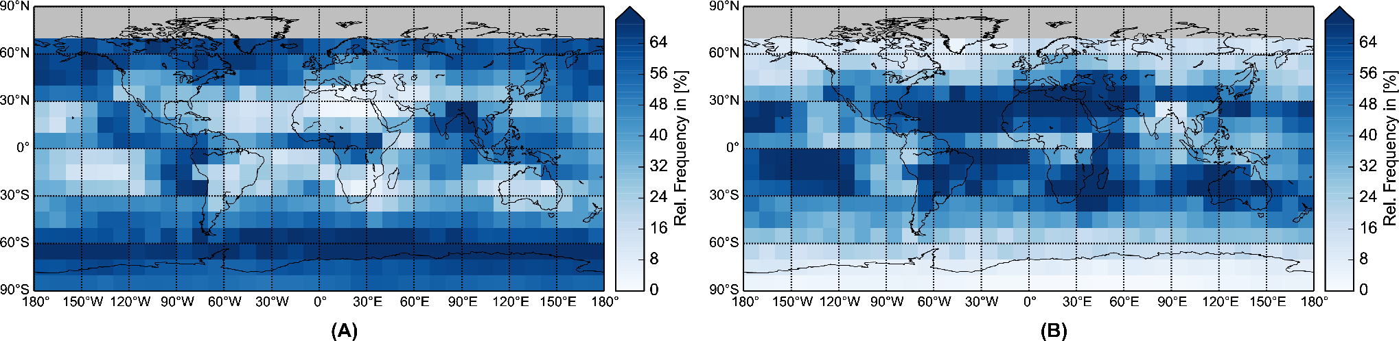
The global distribution of clouds and aerosols detected with high confidence (|CAD |≥ 70) by the CAD algorithm is presented in Figure 2. The global distribution of cloud layers shows a distinct pattern for August 2006–2013. The presence of the intertropical convergence zone and its shifted position due to the monsoon season is visible as clouds occur more frequently along a band north of the equator and at 15° N (Indian subcontinent) [32]. Furthermore, increased relative frequencies are apparent at latitudes from 50° to 70° on both hemispheres. These results are congruent with an analysis by [13] showing the zonal distribution of cloud and aerosol features in July 2006.
When comparing cloud occurrence frequencies to those of aerosols (Figure 2B) an opposite pattern becomes apparent. During August, atmospheric particles dominate lower latitudes of both hemispheres. Emission sources such as the Saharan desert, Australia, South Africa and Brazil can be recognized. Biomass burning aerosols, mineral dust and sea spray are the main contributors to the aerosol loading above southern-hemispheric oceans during August [13]. Northern hemisphere aerosols are primarily composed of mineral dust next to sulfate, organic aerosols and nitrate from anthropogenic sources in South East Asia, United States and Europe [33,34]. The CAD algorithm is able to classify multiple layers, but only as either cloud or aerosol. As long as both features occur, e.g., in a mixed layer, the confidence decreases and the feature is assigned to the most likely class (Section 2). Thus, aerosols are apparently absent in regions where clouds frequently occur due to the fact that optically thin aerosol layers or those features obscured by overlying optically thick clouds cannot be detected [25].
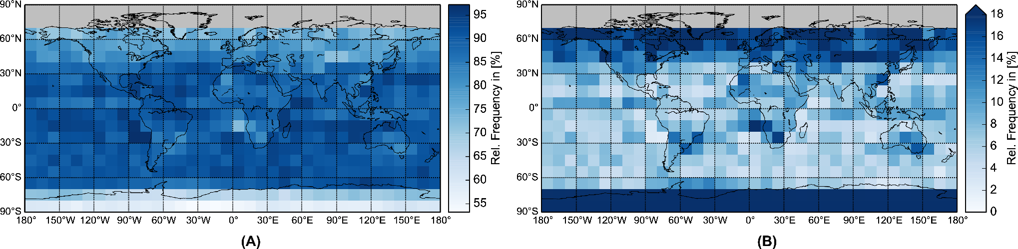
Figure 3A shows the sum of aerosol and cloud relative frequencies, illustrating that on a global scale, most features are assigned to these two classes (global mean sum of relative frequencies: 86%). Still, regions (40°–70°N, 70°–90°S and equatorial Pacific) can be identified where relative frequencies are lower.
Counting only the occurrences of NCR features (5.98% of the total CAD range from −100 to 100) reveals a visual counterpart to Figure 3A and is shown in panel (B). Most of the high frequencies are found in exactly the same regions where they were reduced in Figure 3A.
With the filter application, a total of 70.6% of NCR features were removed from the data. The relative data loss corresponding to each single filter is reported in Table 2.
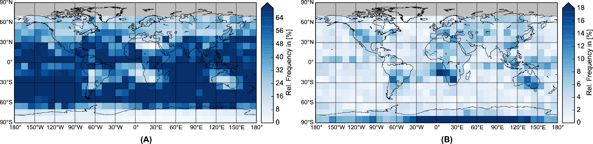
Due to the application of the IAB filter, ∼70% of the NCR data with the potential of containing hydrated aerosols under optically thick features are removed and cannot be considered in the analysis. As a consequence, only hydrated aerosols under thin layers or clear conditions are included in the NCR. The global effect of the IAB filter on the NCR data is illustrated in Figure 4A. Features with overlying layers show a distinct pattern of low relative frequencies in Southern Africa, South America, Australia and the Mediterranean.
After application of all filters a global pattern as shown in Figure 4B emerges. The South-East Atlantic stands out with relative frequencies of up to 20%, the South Pole between 80° and 90° S with up to 36%. Apart from these regions, relative frequencies above 10% mostly occur above the continents and near the equator.
4. Discussion
The NCR may contain a variety of features along with classification artifacts. Therefore, the global pattern of NCR occurrence frequencies (Figure 4B) reflects both, artifacts and physical properties of atmospheric features [13,20,31]. While the last case is pursued, it is impossible to remove all artifacts with confidence. Applying stricter filter thresholds would likely result in the loss of meaningful data. Accordingly, features with an IAB QA ≥ 0.7 are not filtered out.
In order to untangle physical features from artifacts, and to assess the filters, Figure 5A–C shows the five CAD dimensions of the NCR after filtering. As can be seen in panel (A), most of the features of the NCR pixels are not centered on the AB-CR region between pure aerosol and pure cloud features (white box). The attenuated backscatter and particles size of hydrated aerosols should in most cases be larger than for dry aerosols due to water uptake [35,36]. One group of layers assigned a CAD value in the NCR are found at CR < 0.7 and between an AB of ∼10−3.5 and ∼10−2.5 km−1 · sr−1. These are the typical ranges within which molecular scattering and aerosol signals are found (see Section 2). The aerosol cluster (Figure 1A) and many of the NCR features (Figure 5A) lie in nearly the same 2D space. This pattern is favored by the CAD algorithm, which is biased towards classifying uncertain features as cloud in order to avoid cloud contamination in aerosol retrievals [21]. This means that a large portion of hydrated aerosols are probably classified as clouds.
Features far from the aerosol and cloud clusters become apparent, having uncertain physical and optical properties (e.g., the features with a CR close to zero and a large AB). These features are generated due to retrieval artifacts as originating from overlying optical thick features, due to noise in the signal or multiple scattering effects [13], but could not be filtered out completely. The area with a CR > 1.0 and an AB of ∼10−2.5 km−1 · sr−1 might be associated with optically thin clouds and dust layers under humid conditions, whereas maritime aerosols (90% relative humidity) occur at a CR of ∼0.7 [25,30]. In addition, optically thick smoke can be characterized by large CR due to large differences in the extinction of 532 and 1064 nm and can compose features of the NCR [37].
Dense dust and smoke plumes misclassified as cloud may fall into the NCR, especially when they are transported to higher latitudes where cirrus clouds occur at lower altitudes. Very dense dust and smoke layer over the source regions and dense open-ocean aerosols are correctly classified as aerosols. Only very dense parts of the layer detected at single-shot (333 km) resolution are automatically classified as cloud and are not further considered by the CAD algorithm [18,20]. This is especially true for small parts of dense smoke plumes [38]. Thus, biomass burning particles originating from South African and American sources may cause misclassifications affecting the relative frequencies of NCR features presented in Figure 4B. Instead, the Saharan dust belt prevailing during August over the Atlantic Ocean around 20°N [23] is not visible, implying the correct classification of dense dust to the aerosol class. This is supported by the distribution of NCR features in the DR-AB space (Figure 5B). The DR has a value close to zero after the application of the filters, indicating the presence of non-dust aerosols or thin dust layers and molecular scattering [28,37].
A comparison of Figures 5B and 1B shows that ice particles and water clouds (high DR and AB) are not present in the NCR. Nevertheless, a low depolarization in combination with a relatively low AB can suggest the presence of polar stratospheric clouds (PSCs) south of 70° S (Figure 4B). They are probably composed of a mixture of ice crystals and super-cooled ternary solution droplets formed by condensational growth of background stratospheric aerosols [25,39]. Their distinct characteristics compared to ice clouds at lower latitudes add uncertainties to the separation of aerosols and clouds by the CAD algorithm, especially when they are optically thin, low-lying and spatially diffuse [13,20]. Cirrus clouds mixed with dust/smoke particles might be responsible for misclassifications of clouds and aerosols by CALIPSO’s CAD score due to increased emission during this time [13,18,20].
Apparently, the presence of these features in the NCR would suggest their occurrence below the tropopause and thus they could not be filtered from the data set. Figure 5C shows that large parts of features in the NCR are located at lower latitudes and below an altitude of 2 km. At the South Pole NCR features with an average top altitude of 4.9 km can be found. The part of polar clouds that could not be excluded from the NCR might explain the remarkable pattern between 80° and 90° S during August as found in Figure 4. Removing all objects south of 70° S as in Figure 6C reveals scattering characteristics of NCR objects above a CR of 0.5, between an AB of ∼10−3 and ∼10−2 km−1 · sr−1 and a DR which varies from 0 to 0.1 (Figure 6A,B).
Accordingly, the remaining NCR features (polar clouds south of 70°S left beyond) may be non-dust aerosols not well identified by the CAD algorithm like optically thick smoke, hydrated aerosols or optically thin clouds.
5. Conclusions
The focus of the study was on evaluating the potential to derive global occurrence frequencies of features between clouds and aerosols based on CALIPSO’s cloud-aerosol discrimination product. As the CAD no-confidence range may contain a variety of features other than hydrated aerosol [13], their number was reduced explicitly by using filters, with the aim of retaining only hydrated aerosols.
The global distribution obtained for the August test case shows spatial patterns largely consistent with expectations, with high frequencies in regions with high aerosol emissions. After applying the filters, features show an AB of ∼10−2.5 km−1 · sr−1, a CR of ∼0.6 and >1.0, indicative of hydrated aerosols, very dense aerosol layers or thin clouds. In general, most of the features are located below 2 km, which would appear plausible for hydrated aerosol.
Atmospheric objects in the NCR are not consistently located between clouds and aerosols in terms of attenuated backscatter and color ratio. However, hydrated aerosols may display scattering characteristics outside of this overlap region similar to cloud and aerosol properties depending on their hydration state. The CAD algorithm is biased in that uncertain pixels tend to be classified as cloud in order to allow for uncontaminated aerosol retrievals [21,25]. Accordingly, hydrated aerosols are likely classified as cloud in many cases.
The filters implemented work well for the exclusion of ice features and, with restrictions, for layers overlain by optically thick features. Still, features with unknown phase and origin such as PSCs and parts of dense smoke layers remain in the data set. Nevertheless, the global distribution of retained features shows a plausible pattern, with scattering properties implying an early hydration state of aerosols.
While a portion of hydrated aerosol pixels of unknown size is likely classified as cloud by the CAD, the results still indicate that NCR may be useful in determining regions where aerosol processing by clouds takes place.
Acknowledgments
The authors are grateful to the CALIPSO Science Team for their efforts, and for making data products available. The CALIPSO data were obtained from the NASA Langley Research Center Atmospheric Science Data Center. Funding for this study was provided by Deutsche Forschungsgemeinschaft (DFG) in the project GEOPAC (grant CE 163/5-1). The authors thank Hendrik Andersen for helpful discussions. The constructive comments of four anonymous reviewers greatly helped to improve the manuscript.
Author Contributions
Julia Fuchs and Jan Cermak conceived the study; Julia Fuchs designed the methodology, performed the computations, analysed the findings and wrote the paper; Jan Cermak provided methodological support, contributed to the interpretation of the results, style and expression.
Conflicts of Interest
The authors declare no conflict of interest.
References
- Koren, I.; Feingold, G. Aerosol-cloud-precipitation system as a predator-prey problem. Proc. Natl. Acad. Sci. USA 2011, 108, 12227–12232. [Google Scholar]
- Feingold, G.; Siebert, H. Cloud-aerosol interactions from the micro to the cloud scale. In Clouds Perturbed Climate System Their Relatship to Energy Balance Atmospheric Dynamics, and Precipation; Heintzenberg, J., Charlson, R.J., Eds.; MIT Press: Cambridge, MA, USA; London, UK, 2009; Chapter 14; pp. 319–338. [Google Scholar]
- Altaratz, O.; Koren, I.; Remer, L.; Hirsch, E. Review: Cloud invigoration by aerosols—Coupling between microphysics and dynamics. In Atmos. Res.; 2014; Volume 140–141, pp. 38–60. [Google Scholar]
- McComiskey, A.; Feingold, G.; Frisch, A.S.; Turner, D.D.; Miller, M.A.; Chiu, J.C.; Min, Q.; Ogren, J.A. An assessment of aerosol-cloud interactions in marine stratus clouds based on surface remote sensing. J. Geophys. Res. 2009, 114. [Google Scholar] [CrossRef]
- Andreae, M.O.; Rosenfeld, D. Aerosol-cloud-precipitation interactions. Part 1. The nature and sources of cloud-active aerosols. Earth Sci. Rev. 2008, 89, 13–41. [Google Scholar]
- Jeong, M.J.; Li, Z. Separating real and apparent effects of cloud, humidity, and dynamics on aerosol optical thickness near cloud edges. J. Geophys. Res. 2010, 115. [Google Scholar] [CrossRef]
- Boucher, O.; Randall, D.; Artaxo, P.; Bretherton, C.; Feingold, G.; Forster, P.; Kerminen, V.M.; Kondo, Y.; Liao, H.; Lohmann, U.; et al. Clouds and Aerosols. In Climate Change 2013: The Physical Science Basis, Contribution of Working Group I to the Fourth Assessment Report of the Intergovernmental Panel on Climate Change; Stocker, T.F., Qin, D., Plattner, G.K., Tignor, M., Allen, S.K., Boschung, J., Nauels, A., Xia, Y., Bex, V., Midgely, P.M., Eds.; Cambridge University Press: Cambridge, UK; New York, NY, USA, 2013. [Google Scholar]
- Eck, T.F. Variability of biomass burning aerosol optical characteristics in southern Africa during the SAFARI 2000 dry season campaign and a comparison of single scattering albedo estimates from radiometric measurements. J. Geophys. Res. 2003, 108. [Google Scholar] [CrossRef]
- Wang, X.; Huang, J.; Ji, M.; Higuchi, K. Variability of East Asia dust events and their long-term trend. Atmos. Environ. 2008, 42, 3156–3165. [Google Scholar]
- Painemal, D.; Zuidema, P. Microphysical variability in southeast Pacific Stratocumulus clouds: synoptic conditions and radiative response. Atmos. Chem. Phys. 2010, 10, 6255–6269. [Google Scholar]
- Koren, I.; Remer, L.A.; Kaufman, Y.J.; Rudich, Y.; Martins, J.V. On the twilight zone between clouds and aerosols. Geophys. Res. Lett. 2007, 34, 1–5. [Google Scholar]
- Koren, I.; Oreopoulos, L. How small is a small cloud? Atmos. Chem. Phys. 2008, 8, 3855–3864. [Google Scholar]
- Liu, Z.; Vaughan, M.; Winker, D.; Kittaka, C.; Getzewich, B.; Kuehn, R.; Omar, A.; Powell, K.; Trepte, C.; Hostetler, C. The CALIPSO Lidar cloud and aerosol discrimination: Version 2 algorithm and initial assessment of performance. J. Atmos. Ocean. Technol. 2009, 26, 1198–1213. [Google Scholar]
- Charlson, R.J.; Ackerman, A.S.; Bender, F.A.M.; Anderson, T.L.; Liu, Z. On the climate forcing consequences of the albedo continuum between cloudy and clear air. Tellus B 2007, 59, 715–727. [Google Scholar]
- Loeb, N.G.; Schuster, G.L. An observational study of the relationship between cloud, aerosol and meteorology in broken low-level cloud conditions. J. Geophys. Res. 2008, 113. [Google Scholar] [CrossRef]
- Su, W.; Schuster, G.L.; Loeb, N.G.; Rogers, R.R.; Ferrare, R.A.; Hostetler, C.A.; Hair, J.W.; Obland, M.D. Aerosol and cloud interaction observed from high spectral resolution Lidar data. J. Geophys. Res. 2008, 113. [Google Scholar] [CrossRef]
- Yang, W.; Marshak, A.; Várnai, T.; Liu, Z. Effect of CALIPSO cloudâĂ Şaerosol discrimination confidence levels on observations of aerosol properties near clouds. Atmos. Res. 2012, 116, 134–141. [Google Scholar]
- Trepte, C.R. CALIPSO—Data User’s Guide—Data Product Descriptions, Available online: http://www-calipso.larc.nasa.gov/resources/calipso_users_guide/data_summaries/layer/index.php#cad_score accessed on 1 December 2014.
- Trepte, C.R. CALIPSO—Data User’s Guide—Frequently Asked Questions, Available online: http://www-calipso.larc.nasa.gov/resources/calipso_users_guide/faq.php accessed on 1 December 2014.
- Liu, Z.; Kuehn, R.; Vaughan, M.; Winker, D. The CALIPSO Cloud and Aerosol Discrimination: Version 3 Algorithm and Test Results, Proceeding of 25th International Laser Radar Conference (ILRC), St. Petersburg, Russia, 5–9 July 2010.
- Winker, D.M.; Vaughan, M.A.; Omar, A.; Hu, Y.; Powell, K.A.; Liu, Z.; Hunt, W.H.; Young, S.A. Overview of the CALIPSO mission and CALIOP data processing algorithms. J. Atmos. Ocean. Technol. 2009, 26, 2310–2323. [Google Scholar]
- Costantino, L.; Bréon, F.M. Aerosol indirect effect on warm clouds over South-East Atlantic, from co-located MODIS and CALIPSO observations. Atmos. Chem. Phys. Discuss. 2012, 12, 14197–14246. [Google Scholar]
- Kaufman, Y.J.; Koren, I.; Remer, L.A.; Tanré, D.; Ginoux, P.; Fan, S. Dust transport and deposition observed from the Terra-Moderate Resolution Imaging Spectroradiometer (MODIS) spacecraft over the Atlantic Ocean. J. Geophys. Res. 2005, 110, 1–16. [Google Scholar]
- Vaughan, M.A.; Young, S.A.; Winker, D.M.; Powell, K.A.; Omar, A.H.; Liu, Z.; Hu, Y.; Hostetler, C.A. Fully automated analysis of space-based Lidar data: An overview of the CALIPSO retrieval algorithms and data products. Proc. SPIE 2004, 5575, 16–30. [Google Scholar]
- Liu, Z.; Omar, A.; Hu, Y.; Vaughan, M.; Winker, D. Part 3: Scene Classification Algorithms, Available online: http://ccplot.org/pub/resources/CALIPSO/CALIOP%20Algorithm%20Theoretical%20Basis%20Document/PC-SCI-202.03%20Scene%20Classification%20Algorithms.pdf accessed on 1 December 2014.
- Hostetler, C.A.; Liu, Z.; Reagan, J. Calibration and Level 1 Data Products, Available online: http://calipsovalidation.hamptonu.edu/PC-SCI-201v1.0.pdf accessed on 1 December 2014.
- Vaughan, M.A.; Winker, D.M.; Powell, K.A. Part 2: Feature Detection and Layer Properties Algorithms, Available online: http://calipsovalidation.hamptonu.edu/PC-SCI-202_Part2_rev1x01.pdf accessed on 1 December 2014.
- Omar, A.H.; Winker, D.M.; Vaughan, M.A.; Hu, Y.; Trepte, C.R.; Ferrare, R.A.; Lee, K.P.; Hostetler, C.A.; Kittaka, C.; Rogers, R.R.; et al. The CALIPSO automated aerosol classification and Lidar ratio selection Algorithm. J. Atmos. Ocean. Technol. 2009, 26, 1994–2014. [Google Scholar]
- Hu, Y.; Winker, D.; Vaughan, M.; Lin, B.; Omar, A.; Trepte, C.; Flittner, D.; Yang, P.; Nasiri, S.L.; Baum, B.; et al. CALIPSO/CALIOP cloud phase discrimination algorithm. J. Atmos. Ocean. Technol. 2009, 26, 2293–2309. [Google Scholar]
- Liu, Z. Use of probability distribution functions for discriminating between cloud and aerosol in lidar backscatter data. J. Geophys. Res. 2004, 109, D15202. [Google Scholar]
- Trepte, C.R.; CALIPSO—Quality, Statements; Lidar, Level. 2 Vertical Feature Mask Product Version Releases: 3.01, 3.02, Available online: https://eosweb.larc.nasa.gov/sites/default/files/project/calipso/quality_summaries/CALIOP_L2VFMProducts_3.01.pdf accessed on 1 December 2014.
- Patra, P.; Behera, S. The Indian summer monsoon rainfall: Interplay of coupled dynamics, radiation and cloud microphysics. Atmos. Chem. Phys. 2005, 5, 2181–2188. [Google Scholar]
- Zhang, X.Y.; Wang, Y.Q.; Niu, T.; Zhang, X.C.; Gong, S.L.; Zhang, Y.M.; Sun, J.Y. Atmospheric aerosol compositions in China: Spatial/temporal variability, chemical signature, regional haze distribution and comparisons with global aerosols. Atmos. Chem. Phys. 2012, 12, 779–799. [Google Scholar]
- Jimenez, J.; Canagaratna, M. Evolution of organic aerosols in the atmosphere. Science 2009, 326, 1525–1529. [Google Scholar]
- Feingold, G.; Morley, B. Aerosol hygroscopic properties as measured by Lidar and comparison with in situ measurements. J. Geophys. Res. 2003, 108. [Google Scholar] [CrossRef]
- Freney, E.J.; Adachi, K.; Buseck, P.R. Internally mixed atmospheric aerosol particles: Hygroscopic growth and light scattering. J. Geophys. Res. 2010, 115. [Google Scholar] [CrossRef]
- Liu, Z.; Liu, D.; Huang, J.; Vaughan, M.; Uno, I.; Sugimoto, N.; Kittaka, C.; Trepte, C.; Wang, Z.; Hostetler, C.; Winker, D. Airborne dust distributions over the Tibetan Plateau and surrounding areas derived from the first year of CALIPSO Lidar observations. Atmos. Chem. Phys. Discuss. 2008, 8, 5957–5977. [Google Scholar]
- Wu, Y.; Cordero, L.; Gross, B.; Moshary, F.; Ahmed, S. Assessment of CALIPSO attenuated backscatter and aerosol retrievals with a combined ground-based multi-wavelength Lidar and sunphotometer measurement. Atmos. Environ. 2014, 84, 44–53. [Google Scholar]
- Lowe, D.; MacKenzie, A.R. Polar stratospheric cloud microphysics and chemistry. J. Atmos. Sol. Terr. Phys. 2008, 70, 13–40. [Google Scholar]


| Measure | Aerosols | Water Clouds | Ice Clouds |
|---|---|---|---|
| AB | ~10−3 km−1 · sr−1 | ~10−1 km−1 · sr−1 | ~10−2 km−1 · sr−1 |
| CR | ~0.45 | ~0.95 | ~1.0 |
| DR | ~0.02–0.05 | ~0.2 | ~0.25–0.4 |
| Filter | Fraction of NCR [%] |
|---|---|
| IAB | 99.8 |
| Ice | 0.2 |
© 2015 by the authors; licensee MDPI, Basel, Switzerland This article is an open access article distributed under the terms and conditions of the Creative Commons Attribution license (http://creativecommons.org/licenses/by/4.0/).
Share and Cite
Fuchs, J.; Cermak, J. Where Aerosols Become Clouds—Potential for Global Analysis Based on CALIPSO Data. Remote Sens. 2015, 7, 4178-4190. https://doi.org/10.3390/rs70404178
Fuchs J, Cermak J. Where Aerosols Become Clouds—Potential for Global Analysis Based on CALIPSO Data. Remote Sensing. 2015; 7(4):4178-4190. https://doi.org/10.3390/rs70404178
Chicago/Turabian StyleFuchs, Julia, and Jan Cermak. 2015. "Where Aerosols Become Clouds—Potential for Global Analysis Based on CALIPSO Data" Remote Sensing 7, no. 4: 4178-4190. https://doi.org/10.3390/rs70404178