Ground-Level Classification of a Coral Reef Using a Hyperspectral Camera

Abstract

Especially in the remote sensing context, thematic classification is a desired product for coral reef surveys. This study presents a novel statistical-based image classification approach, namely Partial Least Square Discriminant Analysis (PLS-DA), capable of doing so. Three classification models were built and implemented for the images while the fourth was a combination of spectra from all three images together. The classification was optimised by using pre-processing transformations (PPTs) and post-classification low-pass filtering. Despite the fact that the images were acquired under different conditions and quality, the best classification model was achieved by combining spectral training samples from three images (accuracy 0.63 for all classes). PPTs improved the classification accuracy by 5%–15% and post-classification treatments further increased the final accuracy by 10%–20%. The fourth classification model was the most accurate one, suggesting that combining spectra from differ conditions improves thematic classification. Despite some limitations, available aerial sensors already provide an opportunity to implement the described classification and mark the next investigation step. Nonetheless, the findings of this study are relevant both to the field of remote sensing in general and to the niche of coral reef spectroscopy.

1. Introduction

Remotely sensed spectral data analysis has the potential to become a cost-effective practice for large scale reef investigation, assessment, and monitoring (e.g., [1,2,3,4]). Among these applications, the most desired output is an image classification (or thematic mapping) by which researchers can quantify or map substrates in their study area (e.g., [5,6,7]). However, the integrity of marine remotely sensed data may often be compromised due to: (1) environmental effects—the optical effect of the water and air columns (e.g., [8,9,10]); (2) sensor-imposed effects—spatial, spectral, and noise limitations (e.g., [11,12]); and (3) spectral similarities between the reflectance of the different desired substrate (e.g., [5,6,13]).

Due to the very heterogeneous nature of coral reef habitats, spectral classification of this environment becomes inherently difficult. Even the currently available spaceborne systems with spatial resolution of 1–4 m are unlikely to capture “pure”, unmixed pixels [5,14,15]. Concordantly, the substrate combination within a single pixel may not linearly contribute to its overall reflectance pattern [16,17,18]. Studies attempting to address this problem have used a combination of solutions with some success. For example, “subpixel analysis” (e.g., [12]) attempts to estimate the partial contribution of substrates to a single pixel. Another approach is focusing the classification on specific highly detectable substrates such as bleaching [19,20,21,22,23]. Another complementary solution is data combinations from different sources (e.g., [3,13,24,25]). Recently, a variety of advanced statistical approaches based on spectral techniques have been employed [3,13,25,26].

Spectral separability of reef substrates has drawn the attention of many researchers (e.g., [3,5,27]). Most of them have focused on hyperspectral data that benefit from the ability to detect unique spectral features [27,28,29,30,31]. Hyperspectral resolution, defined as imagery with tens to hundreds of bands, requires a different analytical approach to multispectral imagery or digital photography. The high resolution spectrum can be used to “fingerprint” the chemical properties of the substrate. Particular independent absorbance peaks and between-band relationships provide distinctive features that make specific substrate fingerprinting possible. This property of the spectrum makes its analysis different from a chemical analysis based on independent, separate sources of different scales. Therefore, to benefit from this unique structure, the statistical methods chosen for analysis have to account for this complexity. Additional characteristics of hyperspectral datasets include data redundancies. Due to the high co-linearity of spectral data, adjacent bands contain similar information; these bands do not contribute to the characterisation and separability of the spectra. Therefore, only a subset of the bands can be selected for successfully completing any given application. Collecting less data has implications on the overall handling and storage of spectra or an image.

In comparison to the previous attempt at ground-based hyperspectral imagery [26], the current study presents an improved approach for classification, namely the Partial Least Squares-Discriminant Analysis (PLS-DA) procedure. The PLS-DA procedure is particularly suited to handling hyperspectral data, and is based on dimensionality reduction products, such as principle component analysis (PCA) [32,33]. For example, PCA was suggested as a good way to maximise the benefits of the high spectral resolution data sources of coral reefs (e.g., [12,34,35]). PLS-DA, just like the PCA, uses variations in the data to model principle components that can explain the dataset (or predictor X). In this respect, these methods take into account not only the given value of each band but also account for its relationship to its neighbouring bands. Unlike the PLS-DA, PCA implementation is exclusively based on the data without incorporating additional training or grouping data. The training gives PLS-DA a great advantage and the fact that this is categorical non-parametric grouping is both unique and necessary for the task at hand [36,37,38].

An additional and much desired output of the PLS-DA is the variable importance in projection (VIP). As the name suggests, this is a way to estimate the importance of every predictor (in this case, spectral bands) in the grouping of a class [39]. Using the VIP scores, it is possible to narrow down the spectral selection needed to achieve a worthwhile classification. Theoretically, focusing data acquirement on bands that score highly in the VIP will improve the analysis accuracy. Conversely, spectral bands that score poorly on the VIP hold unimportant spectral features and can be omitted from the model-building data.

The accuracy of an image thematic mapping based on a classification model is dependent on the model training spectra. Unlike previous studies that collected spectra using a spectrometer [40,41,42,43], here samples are collected from the image itself. The earlier described inherent discrepancies of underwater remote sensing are represented by the quality of those samples. Using spectral samples from different images offers a unique opportunity to gain insight on how classification is affected by these inconsistencies.

The aim of the study was to assess the use of the ground-level spectroscopy for underwater coral reef classification, and at the same time to address its applicability for coral reef surveying. To fulfil this aim, the classification models were relied on Partial Least Squares-Discriminant Analysis (PLS-DA) procedure, pre-processing transformations (PPTs) were tested, and post-classification low-pass filtering was applied.

2. Methods

2.1. Study Site and Image Acquisition

The Coral Reef Marine Park (29°33′N 34°57′E) is located 8 km south of the city of Eilat at the northern end of Aqaba Bay. The study site is categorized as a fringing reef and is considered to be relatively small (the reef table is approximately 25 m wide and 2 km long). The choice of location was based on the availability of an over-water dry structure and the relatively flat reef table. Three hyperspectral images were obtained from two separate jetties (pedestrian bridges) 500 metres apart (Figure 1) over the same reef stretch. The first image (image 1, Figure 2A) was taken on the southern jetty during spring 2012 while the second and third images (number 2 and 3, Figure 2B,C, respectively) were taken on the northern jetty in the late summer of 2013. The images were acquired during the late morning when the sun was at an angle that minimised the glint effect. Although variations in solar illumination between photos are expected, those are accepted as one of the contributing factors for differences in image environmental conditions. It is these differences in environmental conditions that the combined classification model aims to bridge.

For image 1, the environmental conditions were favourable, with a low northerly wind (approximately 5 knots). The scene was located at the centre of the reef table at low tide, so the average depth of the reef table was 30 cm (ranging from 20 to 50 cm). The acquisition conditions for image 2 were less favourable with 6 knots wind speed (similar to the first image acquisition), but the wind direction was different (easterly), resulting in an enhanced water surface rippling. The scene was at the internal edge of the reef table and included a section of the lagoon (a sandy bottom under a metre of water column). The reef depth varied from 50 cm to over 1 metre in certain areas. Image 3 was acquired on the same day but wind speed had risen to 7 knots. The scene was located within the shallower area of the reef on a rocky-rubbly slope. This meant that the water depth was close to 1 m, and the live cover was very poor. Additionally, the distance between the camera and the object varied greatly, resulting in marked differences in spatial resolution and scene size.

Figure 1. The hyperspectral camera setup over the jetty. The jetty is built about 1.5 m above the reef table. The camera construction was made so it took near nadir images, 3 m above the jetty. Ropes were used to stabilise the entire construction against wind.

Figure 1. The hyperspectral camera setup over the jetty. The jetty is built about 1.5 m above the reef table. The camera construction was made so it took near nadir images, 3 m above the jetty. Ropes were used to stabilise the entire construction against wind.

The camera used was an AISA Spectral Camera HS by Specim Systems Inc. It was fixed on a boom, overhanging the reef as close as possible to the nadir position (Figure 1). The camera’s 28° lens opening, at 2.5 m above the target, captured approximately 2 × 3 m of the reef table, and the acquisition time was nearly 32 s. The camera provides 1600 pixels per line (the image width), giving, on average, 1.25 mm of reef per pixel. Although pixels size is excessively fine for the purpose of this study, it was not resampled into coarser spatial resolution to test how well the PLS-DA coops with illumination and other variation within a substrate unit. Lengthwise, although the camera is able to provide up to 2500 lines, only 1400 of those were captured in order to minimize image distortion at the scan line edges. Since the camera is fairly static while the lens mirror moves (the pushbroom image is captured line by line across the scan direction), the full output image is a long rectangle. It is important to note that the pixels at both ends (lengthways) are taken at an angle causing them to cover a larger surface area than do the pixels at the centre of the image. Spectrally, 849 bands are captured in the spectral range of 400–1000 nm with 0.67–0.74 nm band width. A regular reflex digital camera (producing a commercial standard RGB image) was mounted on the boom and provided a near nadir colour image of the same scene. The digital images (a commercial RGB camera) varied in their quality too and suffered quality-deteriorating effects due to the environmental conditions like waves and surface reflection (although, not to the same extent as the hyperspectral imagery).

Figure 2. Three images used for this study. The images are different in size (scale arrows and quadrate shown), depth in water, variability of cover and conditions. (A–C) show the original images in true colours. (D–F) show the same images with areas of interest (AOIs) selected for modelling (small polygons, dots) and AOIs used for validation (larger polygons). Notice how the image quality and the digital image quality dictate the AOI coverage and thus the capacity for unit validation.

Figure 2. Three images used for this study. The images are different in size (scale arrows and quadrate shown), depth in water, variability of cover and conditions. (A–C) show the original images in true colours. (D–F) show the same images with areas of interest (AOIs) selected for modelling (small polygons, dots) and AOIs used for validation (larger polygons). Notice how the image quality and the digital image quality dictate the AOI coverage and thus the capacity for unit validation.

2.2. Classification

PLS-DA is a relatively new and not (yet) widely used procedure dedicated for high-end, spectra-oriented classification. This procedure is usually applied in conjunction with a comprehensive set of pre-processing options and assessment tools. However, as with other complex and multi-step protocols, it is important to understand which options are available, important, relevant, or applicative than others. Aspects of the PLS-DA protocol were systematically tested but those results are outside the scope of this paper and will be reported elsewhere.

2.3. Image Pre-Processing

The first stage of the image preparation included detecting and converting saturated pixels (due to sun glint) using a dedicated MATLAB code (version 2011a, The Mathworks, Inc., Natick, MA, USA). Saturated pixels were defined as having lost some of the spectral data because those bands have reached above the sensor’s sensitive ceiling. Less than 1% of all pixels were identified as saturated in image 1, but over 5% were saturated in images 2 and 3. To avoid a wide scale masking procedure, these pixels were replaced by averaged values from pixels on either side. The images were then ready for an image pre-processing tool provided by the camera’s manufacturer (AISA Tools). To correct differences of within-camera sensor sensitivity (and sensor noise) a calibration file (‘dark current’) is used in a similar method to dark object subtraction [44,45]. The “dark current” image is collected in situ, before the image itself, provides the necessary calibration details and subtracted from the image—pixel by pixel. Next, the image underwent spectral resampling to 10 nm and the range was trimmed to 25 bands (460–700 nm), which is the spectral range relevant to underwater spectroscopy.

The effect of the water medium on underwater spectra includes scattering by the water air interface layer (e.g., glint), than absorption and scattering by the water column itself. The glint effect is caused by light reflection from the water surface imperfections (e.g., by wavelets) and typically results in overexposure of the effected pixels [46]. Because this is caused by light-source angle to camera it is simple to minimise by careful selection of image acquisition timing and camera angle consideration. Affected pixels are easy to detect and correct because overexposure extends to the near infra-red part of the spectrum (that is usually absorbed by the water column) [46,47]. All overexposed pixels, whether caused by glint or sensor faults, are identified and corrected as described earlier in this section. Correcting the effect of the water column can be one of the most significant steps in underwater image analysis and the methods to do so are numerous [48,49,50,51]. In this study, because the size of every scene is small, water column effect across the scene is generally estimated to be even and very shallow (<1 m). That meant that water correction is small and can be applied to the entire image uniform. Based on these initial assumptions, image water correction relied on underwater reef-level white referencing plate and a dark object to undertake standard empirical line correction [26]. Dividing the image by an extract (spectrum from an averaged area of interest (AOI)) of the underwater white reference plate converts all values into reflectance [44,45]. If the white plate is at the same depth as the reef and affected by the water column in the same way, it is expected to correct the water column effect at the same time.

The final step of image pre-processing was georeferencing, a procedure that includes downscaling. As a baseline, the georeferencing used the approximate true location of the image based on an aerial image. The original geometric scale, different for the three images, was based on the quadrate dimensions (visible in the image) of 1 × 1 m (the typical root mean square error (RMSE) was smaller than 0.1%). The spatial resolution was set at 1 mm for all images and used the ‘nearest neighbour’ method for downscaling which avoids spectral mixing and preserves the pixel spectral content unchanged.

2.4. Reference Map Used for Validation

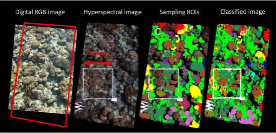
Figure 3 demonstrates all the steps supporting this process for image 1. Each image was carefully examined, together with the digital camera image (Figure 3A), to identify the different substrates on the hyperspectral image (Figure 3B). Images were digitised using the polygon-creating tool in the ENVI image processing software (Environment for Visualizing Images by Research Systems, Inc. version 5.0) and named appropriately by the recognized substrate (Figure 3C). As with an underwater photographic survey, areas in the image were digitised ‘globally’, thus ignoring shaded areas or complexities inside the identified unit. This is particularly relevant when considering complex or multi-layered units such as branching coral. Verification of the classification results was implemented by comparing, pixel by pixel, the classification image with the reference map. The overall accuracy and the Kappa coefficient [52,53] were calculated based only on those pixels with a verification-classification value.

Figure 3. A visual example of image preparation stages demonstrated in image 1. (A) True colour image used for initial referencing and empirical identification. (B) Raw hyperspectral image. (C) AOIs identified in the image divided into two main groups: Samples for the classification model building (small AOIs, dots) and the larger AOIs used for validation. (D–F) are the reference maps used to validate the three classification resolutions (15, 10, and 6 classes, respectively).

Figure 3. A visual example of image preparation stages demonstrated in image 1. (A) True colour image used for initial referencing and empirical identification. (B) Raw hyperspectral image. (C) AOIs identified in the image divided into two main groups: Samples for the classification model building (small AOIs, dots) and the larger AOIs used for validation. (D–F) are the reference maps used to validate the three classification resolutions (15, 10, and 6 classes, respectively).

The digital image was markedly clearer than the hyperspectral one because the digital reflex camera exposure time is a fraction of that of the hyperspectral image. By visually inspecting the digital camera image, it was usually easy to identify growth patterns, colour, and coral genera. This allowed higher identification potential, and the original class designations included growth patterns and genera—two additional subdivisions that were not used for classification in this study.

2.5. Image Analysis

All image analyses were undertaken by the PLS Toolbox 6.7.1 (Eigenvector Research, Inc.: Wenatchee, WA, USA) running on a MATLAB platform. Outputs were exported into Microsoft Excel 2010 for confusion matrices calculations. Image analysis and AOI collection were implemented using ENVI software. As a pioneering study that uses the PLS Toolbox in the coral reef environment, many trials were undertaken to fine-tune the data preparation, modelling, and verification options available.

2.5.1. Classification Models

To build a classification model, samples of spectra were acquired from the images. The model-making sampling strategy aimed at representing an example of each and every marine substrate in the three images. For this, between 20 and 50 individual sample AOIs, representing every recognisable substrate existing in the image, were marked (Figure 2D–F). Each of these sample AOIs was made out of 300–1000 pixels, and all pixels in a sample were averaged into a single spectrum. In total, from the three images, 2012 separate spectra were exported into MATLAB’s PLS Toolbox. Spectra that seemed to be particularly dark or whose pureness was doubted were discarded so the final spectra to be used were reduced to 1954. All classes related to the human-made components (white references, frame, etc.) were ignored.

2.5.2. Cross Validation

PLS Toolbox classification model building offers an ‘internal’ model validation output. First, the model’s protocol divided the data into calibration data used for modelling and validation data to which the model was applied and with which the accuracy was assessed. In this protocol the spectra from each class are randomised and every seventh spectrum is selected as “validation”. The model output also includes the Root Mean Square Error of Validation (RMSEV) value along with the Root Mean Square Error of Calibration (RMSEC which includes in the model both calibration and validation data) value. Their values can be set against LVs and give an indication of how each performs separately. This calibration-validation step is referred to as ‘cross-validation’ and essentially gives an indication of the model’s accuracy and robustness.

2.5.3. Model Application

The model application focused on testing how well models trained for one set of conditions can be applied to other sets and conditions. Successful generalization of a spectral classification model determines the relevance of this tool for reef surveys at varied sites. To test this, variations of classification models were created and cross-applied to the three images.

First, classification models 1, 2, and 3 were trained using spectra extracted from the respective images only (images 1, 2, and 3), while classification model 4 was a combination of samples from these three images. The models were applied to their contributing images, and then classification model 4 was applied to each of the three images.

Pre-processing transformations (PPTs): the effect on accuracy of two carefully selected PPTs (normalization and generalised least squares (GLS)) was tested on each image. PPT choice was accuracy based systematic testing of 25 different PPTs and their combination but discussing this step outside the scope of this paper.

2.5.4. Classification Variation

Because the images were of different reef areas acquired at different environmental conditions, class identification showed that only a few classes were shared by all three images (e.g., brown coral, shallow turf). Classification model 1 was built with 18 classes, while classification models 2 and 3 included only 14 and 10 classes, respectively. In the combined classification model, all included 22 classes from all three images (only the three variations of soft corals were combined into one).

2.5.5. Class Resolution

This term relates to the number of classes and reflects on the level of substrate definition used in the validation stage. Because classes are spectrally similar and often get misclassified (e.g., dead coral and shallow turf), three levels of classification resolution were formed (Figure 3D–F) based on combining similar classes into one.

The highest classification resolution (“all”) seen in Figure 3D included all the key classes present in the model. The next resolution down was “colour” (Figure 3E) in which all algal-dominated substrates were merged (the number of classes was 16). The name ‘colour’ reflects the fact that all hard coral colours were presented separately. The lowest classification resolution was termed “basic” (Figure 3F) and included a single hard coral class (combined from seven classes). In the validation process, the validation map included the same division/combining rules.

2.5.6. Post-Classification Filtering

All the models of all variations described in this section output an image that is classified pixel by pixel, and the result is often noisy. This noisy output is directly related to the fine image spatial resolution pixel size and most of that misclassification is related to interference at the water surface or water column. Applying a low-pass filter, namely a majority filter [44,54], is a very effective way of resolving this sort of low-level noise. This type of filter is usually used to smooth the data and to remove specks or “salt and pepper” noise (artefacts that are relatively small scaled, often just a single pixel). Mathematically, this is a convolution filter where the value of the central pixel is replaced by the value of the surrounding pixels (most common value). This is done at a user-specified window size (kernel). After classification, the low-pass filtering was applied with a kernel window of 21 pixels and accuracy assessment for all outputs was identical.

3. Results

3.1. General Overview

All images received identical treatment and can be viewed in Figure 2. The images are different in many ways—complexity, lighting conditions, and spatial resolution (and, to some degree, in depth). Due to the differences in image quality, the digitisation and identification of substrates in image 2 and 3 are less complete than in image 1. Initial digitisation identified over 40 different class entities in image 1. These included the classifications of growth forms and the genera of coral (e.g., brown coral was divided into three growth forms: branching, encrusting, and massive). For the model building, the 40 classes were amalgamated into 20 more general classes but these were simplified further post-classification into the 14 classes used for validation (Figure 4). Seven coral colours were present in image 1 (purple, blue, green, yellow, brown, pink, and white). The choice of breaking the coral class into separate colours was shown to improve the classification and, therefore, was adopted as a classification strategy [3]. Overall, image 1 contributed 1458 different samples to the model (19 classes). Image 2 had only 18 different classes identified within it (but included four classes not present in the other images) and contributed 491 samples to the model. Image 3 was located in the lagoon (deeper and less complex); it included only 10 classes and contributed only 200 samples for classification modelling. The total number of samples used for the combined model was 2211.

Figure 4. Endmember spectral reflectance of key substrate. Similarity between classes is evident and the PTTs offer separation enhancements in those cases.

Figure 4. Endmember spectral reflectance of key substrate. Similarity between classes is evident and the PTTs offer separation enhancements in those cases.

3.2. Model Application

This part of the results includes three planes of examinations based on data and image choices. The results represent combinations of the following variables—three images; four models; two PPTs; two post processing filtering and two measures of accuracy (Table 1). Altogether, 88 classification-image combinations were tested, producing 176 accuracy measurements. However, there is a strong correlation between the overall accuracy and the Kappa coefficient (R² = 0.9), which generally indicates that these results are complimentary. To simplify the results from here on, only the overall accuracy will be reported (n = 88).

Generally, the combined model performed better than either of the image-specific models alone (model accuracy 0.93 Figure 5). Furthermore, when cross applied (i.e., sampling and application not the same), the combined classification model performed slightly better than the classification model based on images 1 and 2 alone. To highlight the effects of key treatment-combinations, accuracy results of the application of the combined model (n = 36) are presented in Table 1. To evaluate some of those elements and describe their effect on the accuracy, specific results are presented below. Although the results relate to the combined model (classification model 4), they are true for all other modelling combinations.

3.2.1. Pre-processing Transformations

PPTs play an important role in the classification process and conceptually affect the classification as can be seen in the graphic representation of the classification models. Generally, normalisation gave a better performance over GLS especially when the image quality was bad. The normalization accuracy score (average accuracy 0.63) is better than that of the GLS (average accuracy 0.60) in 14 out of 18 comparisons.

3.2.2. Class Resolution

In Table 1, termed “class resolution”, the number categories of classes undergoing the accuracy assessment are presented (“all”—14 classes, “colour”—10 classes, and “basic”—6 classes). As expected, the accuracy improves as the number of classes tested is reduced. A confusion matrix (Figure 5 and Figure 6) highlighted that many of the errors are the result of within-group misclassification (e.g., yellow coral classed as brown coral). The results from those indicated that the classification accuracy is low mostly due to between-group misclassifications (e.g., hard coral classed as soft corals or dead corals).

Table 1. Overall accuracy (OA) scores of two transformations (GLS and normalization) applied to three images for three classification resolution labels—“all” n = 14 classes, “colour” n = 10 classes, and “basic” n = 6 classes. Another subdivision is between the unfiltered image and image after majority filter analysis.

		Image 1		Image 2		Image 3
Transformation		GLS	Normalization	GLS	Normalization	GLS	Normalization
Variation
All (14 class)	Raw image	0.47	0.47	0.3	0.35	0.08	0.29
	Majority filter	0.63	0.63	0.48	0.55	0.1	0.33
Colour (10 class)	Raw image	0.6	0.6	0.45	0.49	0.8	0.81
	Majority filter	0.76	0.75	0.71	0.69	0.98	0.99
Basic (6 class)	Raw image	0.64	0.62	0.53	0.57	0.77	0.81
	Majority filter	0.79	0.79	0.85	0.81	0.99	0.99

Table 1. Overall accuracy (OA) scores of two transformations (GLS and normalization) applied to three images for three classification resolution labels—“all” n = 14 classes, “colour” n = 10 classes, and “basic” n = 6 classes. Another subdivision is between the unfiltered image and image after majority filter analysis.

		Image 1		Image 2		Image 3
Transformation		GLS	Normalization	GLS	Normalization	GLS	Normalization
Variation
All (14 class)	Raw image	0.47	0.47	0.3	0.35	0.08	0.29
	Majority filter	0.63	0.63	0.48	0.55	0.1	0.33
Colour (10 class)	Raw image	0.6	0.6	0.45	0.49	0.8	0.81
	Majority filter	0.76	0.75	0.71	0.69	0.98	0.99
Basic (6 class)	Raw image	0.64	0.62	0.53	0.57	0.77	0.81
	Majority filter	0.79	0.79	0.85	0.81	0.99	0.99

Figure 5. The combined classification-model confusion-matrix. The classification model is very successful in predicting classes. Most classes are well defined and those that are not are usually misclassified within the class type (e.g., bleached coral and turf or yellow and brown coral).

Figure 5. The combined classification-model confusion-matrix. The classification model is very successful in predicting classes. Most classes are well defined and those that are not are usually misclassified within the class type (e.g., bleached coral and turf or yellow and brown coral).

Figure 6. The confusion matrix of the classification model based on samples from image 1 and applied to image 1. This example represents the combination of model and image that achieved the highest accuracy score. Most classes are well defined and those that are not are suspected to be contextually badly defined substrates in the reference map image. This highlights the difficulty of the verification process.

Figure 6. The confusion matrix of the classification model based on samples from image 1 and applied to image 1. This example represents the combination of model and image that achieved the highest accuracy score. Most classes are well defined and those that are not are suspected to be contextually badly defined substrates in the reference map image. This highlights the difficulty of the verification process.

3.2.3. Post-classification Filtering

Scores of unfiltered classification images are always less accurate than those after the low-pass filter (Table 1). This improvement in accuracy is systematic and correlated (R² > 0.93 n = 18). This correlation is generally higher in the higher class resolution (both “all” and “colour”—R² > 0.93 n = 12) than in the lower class resolution (R² > 0.69 n = 6). These trends are true for all other classification combinations tested in this study (e.g., models 1, 2, and 3 applied to their respective images and other cross-application variations).

4. Discussion

Being able to separate coral-like substrates (such as coral, soft coral, fire coral, etc.) from algal cover (the first colonisers of dead coral patches and other stabilised substrates) is the most basic reef health indicator (e.g., [14,21,22]). Therefore even the very coarse separation between reef health indicators, such as corals (including fire and soft corals) from turf surfaces (overall accuracy 0.9), makes this analysis a relevant surveying method. The separation described above is limited to spectral details only and overlooks other desired reef monitoring categories. For example, dead coral is an important category that is currently under the “algea covered” classes. While this is spectrally true, the analysis misses an important detail relevant to temporal changes on the reef—coral mortality. Because spectral separation is not possible here, future attempts should consider object or pattern recognition protocols [55,56] as a secondary classification stage.

The results presented in this study suggest that ground-level hyperspectral imagery can be used to successfully classify most coral reef substrates. Other examples of hyperspectral pure pixel imagery of a marine substrate through water in situ are very rare [18,57] and their spatial resolution is ten-fold larger than that offered here. Spatial resolution on its own is not a stand-alone dimension and is highly related to the substrate complexity. In this study the spatial resolution was not resampled, which left the variability within each substrate unit very high. Most of this variation was illumination (e.g., coral oral discs appear darker than their surrounding ridges or shaded parts of the same substrates). However, some of this variation is spectral and reflects structural details in the substrates. Those often can be misclassified as other substrates. As for the examples above, substrate complexity was simplified to the extent that most of the pixels did contain only one substrate (e.g., 4 key classes at [18]. Moreover, unlike the previous attempt by Caras and Karnieli [26], the classification model tested here is an amalgamation of substrates collected from three images and applied to all three. Subsequently, the study focused on which classification system is the best suited for this task. This study opens the door for further application of this setup and upscaling the classification model with a global spectral library of coral reefs. With that in mind, worldwide investigation of coral reef spectra highlight some of the regional discrepancies of classes in different locations [27] and those should be considered carefully. Spectral diversity within classes used here remains a key challenge for reef substrate classification, although it is shown here that some of this variation can be addressed by post classification class combination (see below).

Four classification models were successfully tested on three images. The key and the most interesting of these is the combined model that is based on spectra collected from all images (Figure 7). Combining data from the three sources of information taken in situ and in very different conditions illustrates the validity of the protocol as a potential global surveying technique. Preliminary tests applying a model from one image (e.g., image 1 alone) to another (e.g., image 2) were found to be less successful than either direct sampling or combining the sampling (data not shown).

Figure 7. Classification model of latent variable (LV) scores of two key transformations. (A,B) show the distribution of training samples on the model’s first two LVs. (C,D) are the same models, only presented as the average and standard deviation for each class. The % contribution of each LV is marked in the labels. (A,C) show the generalized least squares (GLS) treated model, and (B,D) are the normalisation (and mean centring). Point distribution between the left and right figures highlight the difference in distribution approach as driven by the pre-processing used.

Figure 7. Classification model of latent variable (LV) scores of two key transformations. (A,B) show the distribution of training samples on the model’s first two LVs. (C,D) are the same models, only presented as the average and standard deviation for each class. The % contribution of each LV is marked in the labels. (A,C) show the generalized least squares (GLS) treated model, and (B,D) are the normalisation (and mean centring). Point distribution between the left and right figures highlight the difference in distribution approach as driven by the pre-processing used.

4.1. Post-Classification Filtering

Post-processing is an important improvement to unfiltered classification results. While this sort of post classification filtering is a well-accepted method in the field of remote sensing, the application of those in the marine environment is only necessary in this dataset because the spatial resolution is so fine. The images of the marine substrate obtained by the camera were noisier than ones collected on land both because of environmental conditions (e.g., glint) and substrate complexity [58,59]. The spectral similarity of the substrates is greatly exaggerated in these conditions resulting in misclassification (Figure 8). Since the model classes each pixel one at a time, the image is speckled or “peppered” (where the majority of the pixels are correctly classed and some are not), whereas the verification process it is compared against is generalised and designates whole polygons. The low-pass filter is a simple and effective way of rectifying this type of problem and this improvement is correlated to the class resolution (i.e., more classes result in more misclassifications). For example, areas of “dead coral” classification are peppered with shallow turf pixels although the majority of the pixels are classed as dead coral. This is because dead corals, shallow turf, and deep turf are much the same thing: a rock covered with algal growth and thus spectrally similar (Figure 4).

Figure 8. A visual representation of the three class-resolution outputs demonstrated in image 1. The reference maps for 15, 10, and 6 classes are shown in the left, respectively. The normalisation products are shown in the middle. The GLS results are shown in the right. The yellow scale arrow shows the 1 m quadrate. Highlighted in a red frame are three exemplary errors and how they affect the final accuracy. The top frame shows a combination of yellow hard coral and soft coral. It is possible to see that regardless of image preparations, some of the coral is misclassified. The middle frame shows errors such as a confusion of soft coral and dead coral (patches of overexposed rocks) and also a validation error where the lagoon polygon may have been drawn over a patch of reef rock. In the bottom frame, a typical “within-coral” misclassification is seen; yellow coral is misclassified as brown coral.

Figure 8. A visual representation of the three class-resolution outputs demonstrated in image 1. The reference maps for 15, 10, and 6 classes are shown in the left, respectively. The normalisation products are shown in the middle. The GLS results are shown in the right. The yellow scale arrow shows the 1 m quadrate. Highlighted in a red frame are three exemplary errors and how they affect the final accuracy. The top frame shows a combination of yellow hard coral and soft coral. It is possible to see that regardless of image preparations, some of the coral is misclassified. The middle frame shows errors such as a confusion of soft coral and dead coral (patches of overexposed rocks) and also a validation error where the lagoon polygon may have been drawn over a patch of reef rock. In the bottom frame, a typical “within-coral” misclassification is seen; yellow coral is misclassified as brown coral.

4.2. Class Resolution

As expected, when the number of classes is small, the benefit of the filter is limited. For example, misclassification between subclasses (e.g., yellow coral and brown coral) is already rectified as they are combined into the “hard coral” class in the lower class resolution (Figure 8). Since combining classes was performed in the unfiltered stage, this type of error is affected by the kernel window size. The choice of using a kernel size of 21 pixels is based on trial and error (preliminary tests from kernel size 3 × 3 to 91 × 91), and showed the best overall results for these specific images. Therefore, it is possible that testing different sizes would lead to a slightly better accuracy for different image-model combinations. Kernel size filtering is probably related to spectral resolution and its scale to substrate units.

The fact that the accuracy results from all pre-processing treatments are correlated suggests that classification accuracy is mostly determined by image quality. Image quality causes the spectral signatures collected in the image to contain unwanted information (noise and spectral artefacts). For example, from a spatial-resolution perspective, image quality and pixel purity suffer from smearing effects (e.g., by surface wavelets or camera lens curving). Conversely, if the subject unit is complex, pixel purity "dilutes" the spectral features of the entire unit. For example, simply having more dark pixels in a sample may cause the spectral features to be reduced and increase misclassification. Therefore, to some extent, reducing spatial resolution is expected to increase accuracy because larger pixel spectra are an average reflection, thus reducing the effect of noise. Finding the correct spatial resolution balance is perhaps one of the key obstacles for underwater classification. Furthermore it is likely to be site specific because achieving pure pixels is dependent on substrate unit size.

Overall, the main cause of errors in classification was introduced by the verification process using the reference map. The gap between the digitisation approach (“globally digitised” and subjective) and the classification approaches (pixel by pixel, spectral) could explain many of the misclassification errors, as well as the success of the low-pass filter. Units in the image were digitised by marking their perimeter in the same way that photographic quadrate analysis is done. For example, darker or shaded sections within a coral colony are all included within the one unit and designated the same class. This is possible for a human digitiser because unit recognition is done based on experience and includes, besides colour, the complete shape and the substrate pattern. Conversely, the model works independently, pixel by pixel, and designates the class based on spectra alone. Although spectra transformation generally improves the classification of dark areas, these areas are rightfully designated “shade” by the model classification. Edges, gaps, and overlaps between units are also of questionable accuracy because these tend to be left undesignated by the manual image classification. Ultimately, the next stage of classification is object-based so by default verification and filtering will benefit from the none pixel by pixel analysis this method offers. This is discussed later on in more detail.

4.3. The Model

The PLS-DA classification model has provided good accuracy results in comparison to previous work, despite the fact that the images were taken above water. The majority of examples from the literature were taken in vitro or using data simulations and not under in situ conditions. For example, focusing on spectroscopy, in the discrimination between healthy and bleached corals, Holden and LeDrew [60] reached 80% accuracy while Hochberg et al. [27] reached a maximum of 83% for a similar range of substrates. Other remote sensing attempts, using substrate assemblages, achieved 63% accuracy [5], or when applying a nine-class division using the hyperspectral aerial sensor CASI, they achieved 81% accuracy [61]. During some preliminary tests, images were classified using an increasing number of sub-classifications. It seemed that using a low classification resolution (10 or even 6 classes) as an initial training input for a classification model resulted in low accuracy (increased between-class misclassification). Conversely, increasing the classification resolution to 25 or even 30 classes by breaking classes into their growth forms (e.g., brown coral branching, brown coral massive, etc.) did not improve accuracy. The combination of the initial high classification resolution with post-classification merging was the most successful apparatus for accuracy improvement. Bleached coral are easily identified using PLS-DA (class accuracy of 0.97), which is important in reef appraisal and in spotting temporal changes on the reef. In reducing the classification resolution from 14 classes to 10, the first group of classes to be combined are the different turf-related classes (shallow turf, deep turf, dead coral, etc.). In all cases, the effect of the class-combining process results in a marked improvement in accuracy.

The classification tested and presented in this research is unique and was never previously tested in the marine environment. Other classification methods relevant to hyperspectral imagery that are worth testing include random forest [25,62] and Support Vector Machine (SVM) (e.g., [13,56,63]). Random forest is reported mostly with regards to increasing accuracy when spectral resolution increase [13,64] and combined with the uses of indices [62]. Preliminary results conducted on image 1 seem to agree with the observation that when the number of classes is large (e.g., 20 classes), random forest may produce better models. In their study, Rozenstein et al. (2014) compared the two approaches (PLS-DA and random forest) and confirmed that, generally, the latter classification method is more successful. For the preliminary assessment of image 1 SVM was use as a classifier successfully [26]. As suggested earlier, the next step in classification should focus on separating conceptual classes such as dead coral and algae. These are spectrally similar but represent an important shift in substrate change. The solution probably lays in the application of object recognition tools that would separate growth patterns (e.g., [55,56]). A recent review by Huang et al. [63] systematically compares a variety of classifiers using combinations of spectral and semantic features datasets. The demonstrated capabilities may be useful sub-divisions of classes such as brown coral into branching and massive colonies. Filtering with a majority filter could be built-in the classification sequence to give more weight to neighbouring pixels thus reducing misclassification. Using the filter can be viewed as problematic when some pixels are correctly classified (and converted by their surroundings) or when the number of pixels of two classes in a kernel window is similar. In the results presented here, most of the wrongly classified pixels tended to be results of environmental conditions such as glint. In these cases, because the scale ratio between every classification unit (e.g., coral colony) and the pixels size is so high (to the order of 6) the chance of incorrect representation is very small. Moreover, size of the window (21 pixels which is one centimetre) is still in the order of 100 s from the average unit size. Huang et al. [65] reviews and systematically tested a range of classification post-processing (CPP) and makes relevant suggestions for combining object based filtering and relearning approaches. A more sophisticated filtering effort could potentially include a decision tree based on contextual rules, but this is outside the scope and need of this study.

The system described has a few limitations both in its physical applicability and in its analysis. The physical requirement of building a rig over the study site determines the methods limited to those sites that can provide such structures. Conversely, in theory, it is possible to obtain imagery using the combination of remotely controlled vehicles and a non-pushbroom sensor, thereby resolving this limitation. From the analysis perspective, limitations are related to classification failures or difficulties described earlier. Those limitations can be resolved by a combination of methods described here and testing other approaches that provide classification details for the data collected. Providing a good measurement of reef health does not have to be based on classification or thematic mapping. Other options, such as using complexity measures and indices [6,66,67], are suggested, and perhaps combining these outputs with classification would be the way forward. In any case, for the classification to better supply attractive data, some improvements in the available technology are needed. The fact that these details can be extracted in a semi-automated way suggests that with additional development and technical improvement, this technique has the potential to become fully automated.

5. Conclusions

In this study, a hyperspectral camera was used to capture an in situ image of the reef table in Eilat. The results presented here show how the combination of high resolution imagery and high-end statistical classification techniques has the potential for extracting underwater habitat details unachievable to date (up to 63% accuracy with 14 classes). While the ultimate aim was to provide a new surveying technique, several interesting and unique insights have emerged.

The results indicate that combining spectra from different sources improves the model functionality and results in better accuracy (5%–8% improvement over a model based on one source image). The fact that the classification model successfully combined spectra from different sources into one model is an important statement relevant to the potential of using this system globally. Expanding the sampling effort to other sites and conditions should be tested and can be used to strengthen the existing model and asses its transferability.

Using a hyperspectral camera in this setup opens new avenues of research in spectroscopy, image analysis and remote sensing of the coral reef environment. The pre-processing and post-processing steps in this procedure prove to be detrimental to accuracy improvement. For example, the use of PPT to sharpen spectral differences between classes resulted in 5%–15% accuracy increase while the application of post classification has added an additional 10%–20% increase in accuracy. Building on the existing statistical methods discussed here, the development of an automated classification output is encouraging. A standardised thematic product output for surveying and monitoring has the potential to improve accessibility and reduce the necessary manpower. Moreover, it can be done offsite and immediately made available everywhere.

Naturally, the limitations of the current technology should be acknowledged, but it is constantly improving. Multispectral imagery already provides sub-meter resolution, so the balance between spectral and spatial resolution has become an important question for future sensor design. Aerial sensors now provide imagery like used here or better but are not yet widely available. Further work planned for this source of imagery focuses on these key options, including classification automation and more complex classification techniques—for example, testing additional classification models (e.g., random forest) and combining spectra classification with object recognition.