Mapping Robinia Pseudoacacia Forest Health Conditions by Using Combined Spectral, Spatial, and Textural Information Extracted from IKONOS Imagery and Random Forest Classifier

Abstract

The textural and spatial information extracted from very high resolution (VHR) remote sensing imagery provides complementary information for applications in which the spectral information is not sufficient for identification of spectrally similar landscape features. In this study grey-level co-occurrence matrix (GLCM) textures and a local statistical analysis Getis statistic (Gi), computed from IKONOS multispectral (MS) imagery acquired from the Yellow River Delta in China, along with a random forest (RF) classifier, were used to discriminate Robina pseudoacacia tree health levels. Specifically, eight GLCM texture features (mean, variance, homogeneity, dissimilarity, contrast, entropy, angular second moment, and correlation) were first calculated from IKONOS NIR band (Band 4) to determine an optimal window size (13 × 13) and an optimal direction (45°). Then, the optimal window size and direction were applied to the three other IKONOS MS bands (blue, green, and red) for calculating the eight GLCM textures. Next, an optimal distance value (5) and an optimal neighborhood rule (Queen’s case) were determined for calculating the four Gi features from the four IKONOS MS bands. Finally, different RF classification results of the three forest health conditions were created: (1) an overall accuracy (OA) of 79.5% produced using the four MS band reflectances only; (2) an OA of 97.1% created with the eight GLCM features calculated from IKONOS Band 4 with the optimal window size of 13 × 13 and direction 45°; (3) an OA of 93.3% created with the all 32 GLCM features calculated from the four IKONOS MS bands with a window size of 13 × 13 and direction of 45°; (4) an OA of 94.0% created using the four Gi features calculated from the four IKONOS MS bands with the optimal distance value of 5 and Queen’s neighborhood rule; and (5) an OA of 96.9% created with the combined 16 spectral (four), spatial (four), and textural (eight) features. The most important feature ranked by RF classifier was GLCM texture mean calculated from Band 4, followed by Gi feature calculated from Band 4. The experimental results demonstrate that (a) both textural and spatial information was more useful than spectral information in determining the Robina pseudoacacia forest health conditions; and (b) the IKONOS NIR band was more powerful than visible bands in quantifying varying degrees of forest crown dieback.

1. Introduction

Recent cases of increased tree mortality and die-offs triggered by drought and/or high temperature have been documented [1,2,3]. However, the fundamental mechanisms underlying tree survival and mortality during drought remain poorly understood [4]. Based on the decline spiral model [5,6], drought can operate as a trigger that may ultimately lead to mortality of trees that are already under stress (due to causes such as old age, poor site condition, and air pollution).

Identifying the location and extent of forest at risk from damaging agents and processes assists forest managers in prioritizing their planning and operational mitigation activities [7]. Stress in forests displays a variety of symptoms, some of which may be detected by remote sensing [8,9]. Plant symptoms detectable by remote sensing may be attributed to an increase in red reflectance due to lowered chlorophyll absorption, a decrease in near infrared (NIR) reflectance due to reduced cell vigor, or shifting of a red edge position that may be invoked by different types of stress (e.g., water or nitrogen deficit) [10] or by natural development of plants (e.g., phenology changes) [11].

Several studies have focused on using Landsat Thematic Mapper/Enhanced Thematic Mapper Plus (TM/ETM+) and Satellite Pour l’Observation de la Terre (SPOT) data to map the extent and location of forest disturbances from regional to continental scales [12,13,14,15,16,17]. Although the usefulness of remote sensing technology in mapping forest health conditions is widely recognized, forest health conditions are more difficult to detect from space than other forest disturbances, such as fire or clear-cutting [18]. For example, living trees, foliated trees, and the understory are frequently observed in a tree crown dieback stand, which usually results in a mixture of reflectance from living trees and understory.

With recent very high resolution (VHR) satellite imagery, such as QuickBird and IKONOS, forest stress and disease can be detected at a crown level [19], which makes discrimination of individual healthy and diseased trees possible [20]. However, the classification of VHR images suffers from uncertainty of the spectral information because the increase of the intra-class variance and decrease of the inter-class variance lead to a reduced separability in the spectral domain, particularly for spectrally similar classes [21]. For example, in stressed/diseased forest stands, the understory plants (e.g., regeneration forest, shrubs, and grasses) presenting in gaps and open areas may have a similar NIR response to a closed forest canopy. Such a classification challenge may be overcome by using image spatial information, such as semivariogram, edge density, grey-level co-occurrence matrix (GLCM), or differential morphological profiles [22,23,24,25,26]. This is because, as spatial resolution increases, ground objects tend to be represented by several pixels, and thus the spatial characteristics of imagery become increasingly important with respect to spectral information [27]. The GLCM has been used to extract the most popular textural information to describe spatial properties of targets [28]. Many studies using VHR sensors’ data have demonstrated that the GLCM textural features are effective for mapping forest structure or discriminating forest disturbance severity [29,30,31,32].

In order to characterize local spatial distribution patterns, such as the dieback of Robinia pseudoacacia trees frequently distributing along river channels or road lines in the Yellow River Delta (YRD), China [33], Getis statistic (Gi) [34,35], a local indicator of spatial association (LISA) method [36], may be applied. The statistic reflects the information generated with respect to local variation of tree health conditions within patterns of spatial dependence, resulting in a potential to uncover discrete spatial regimes. The potential of the Gi statistic to identify significant spatial dependency in remotely sensed imagery has been documented [37,38,39]. In addition, the change information in Gi statistic applied to multi-date remote sensing data could be used to identify coral reef stress [40], detect sandstorms and desertification [41], map soil moisture [42], and identify a homogenous stable area used for the radiometric vicarious calibration of satellite sensors [43].

Given the potential that textural and spatial features may help reduce the uncertainty associated with the classification of forest health conditions, some commonly-used parametric classification algorithms (such as maximum likelihood classifier) may be inadequate to the additional information provided by VHR image data [44]. The spectral variability of an individual tree (e.g., pixels representing sunlit crown, shaded crown, and the influence of factors such as branches, cones, and tree morphology) restricts the development of a unique spectral signature for tree classification [45]. To overcome the difficulty, data mining and machine learning techniques, such as random forest (RF) classifier [46], have been developed and produced promising results in mapping forest health conditions and extracting forest structure parameters [47,48,49]. RF does not rely on the data distribution assumption (e.g., normality) and is robust to spectral variations caused by high intra-class variability. In recent years, the RF technique has proved to be highly successful in complex remote sensing applications with improved classification accuracies that are comparable to or better than most of the state-of-the-art classifiers such as support vector machines, neural networks, and boosting techniques [50,51,52]. Since the textural and local spatial information has the potential to improving the accuracy of class designation by minimizing intra-class variation [30,53], the overall objective of this study is to assess whether the GLCM and Gi features extracted from IKONOS imagery were effective in determining Robinia pseudoacacia forest health conditions in the YRD, China using RF classifier.

2. Study Area and Datasets

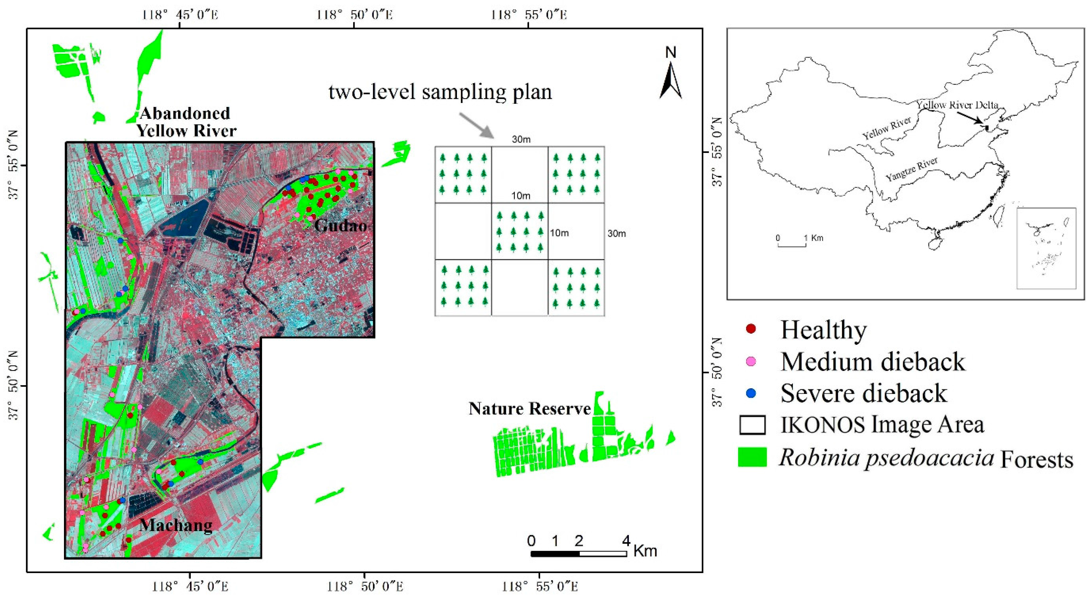
2.1. Study Area

The Yellow River Delta (YRD) is situated in the estuary of the Yellow River in the City of Dongying, Shandong Province of Eastern China (Figure 1). It has a warm temperate, continental monsoon climate with distinctive seasonality. The average annual temperature is 11.7–12.6 °C, and the mean annual precipitation varies between 530 and 630 mm, 70% of which falls during summer. Approximately 10.5 million tons of sand and soil discharged by the river annually are deposited in the delta, forming a vast floodplain and special wetland landscape [54]. The dominant soil types in this area are Calcaric Fluvisols, Salic Fluvisols, and Gleyic Solonchaks. A low groundwater table with a high level of dissolved salts in it and a high evaporation rate (the ratio of the average annual evaporation to precipitation is 3.5:1) make saline soil and secondary saline soil wildly spread. In the YRD, the natural vegetation includes herbs (Viola philippica, Phragmites australis, Setaria viridis, Imperata cylindrica, Aeluropus littoralis, and Phragmites australis, etc.) and shrubs (Salix matsudana and Tamarix chinesis). There are no natural forests in the YRD. Robinia pseudoacacia forests, one of the fast-growing deciduous species in the world, have a certain ability to tolerate drought and soil salinity; therefore they have been planted widely in this area since the 1970s and become the largest artificial forests in China [33]. However, Robinia pseudoacacia forests in the YRD have suffered continuously from dieback and mortality since the 1990s. Besides Robinia pseudoacacia, there are other forest plantations with a relatively small size, including Populus tomentosa, Fraxinus chinesis, Ulmus pumila, and Ailanthus altissima. There are four forest areas in the YRD, including Gudao, Machang, Abandoned Yellow River, and Nature Reserve with a total area of 27.94 km² [33]. Our study area is only part of the Robinia pseudoacacia forest covered by IKONOS imagery in Figure 1.

Figure 1. Location of the study area. The false color composite image covering the Robinia pseudoacacia forests in the study area was made with IKONOS NIR band/Red band/Green band vs. R/G/B. A two-level sampling design (plan) was adopted for a ground survey of forest crown conditions. The color dots in the color composite image show the locations of the sampling plots for three health conditions of Robinia pseudoacacia forests.

Figure 1. Location of the study area. The false color composite image covering the Robinia pseudoacacia forests in the study area was made with IKONOS NIR band/Red band/Green band vs. R/G/B. A two-level sampling design (plan) was adopted for a ground survey of forest crown conditions. The color dots in the color composite image show the locations of the sampling plots for three health conditions of Robinia pseudoacacia forests.

2.2. Datasets

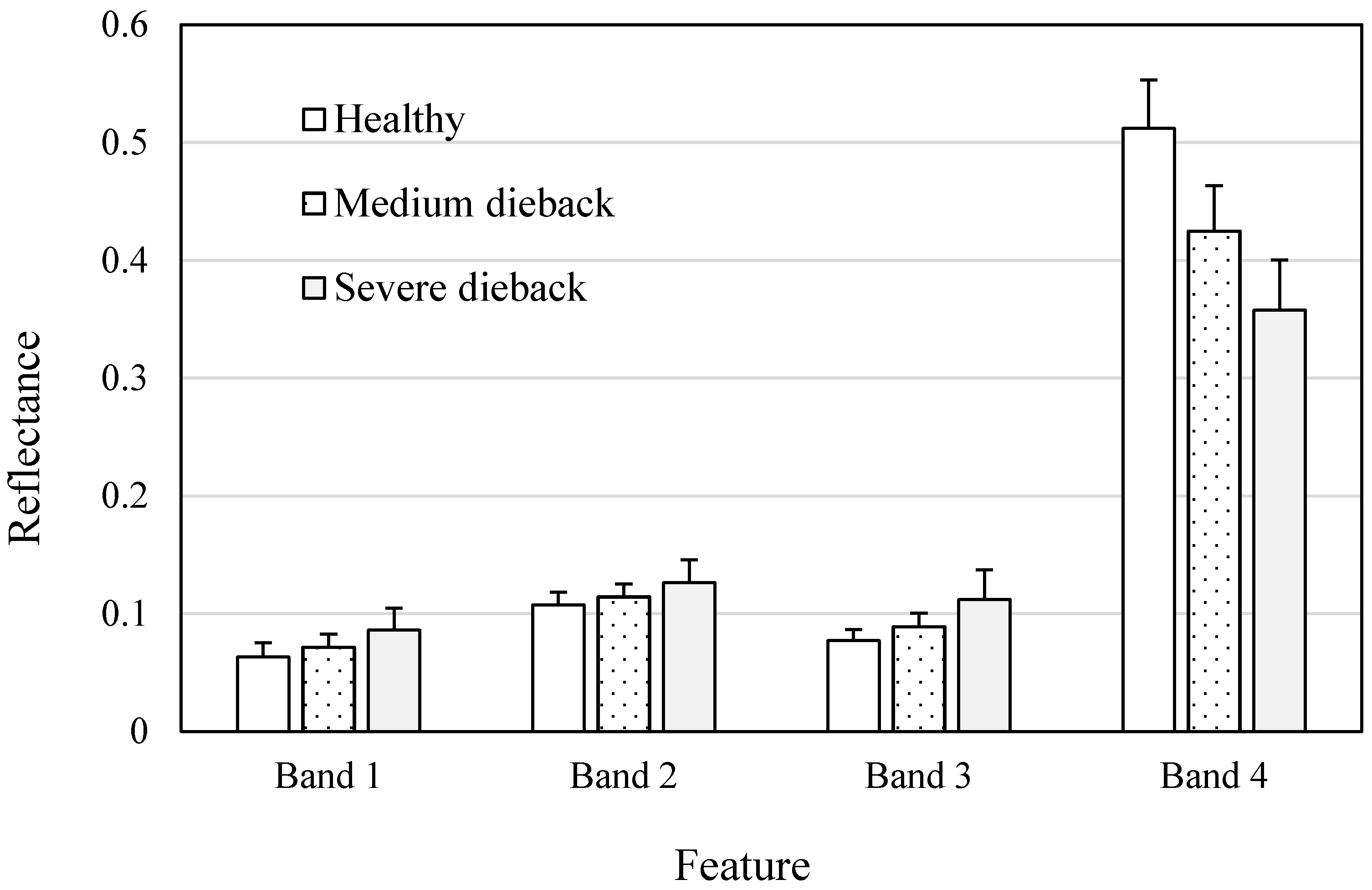
2.2.1. Satellite Imagery

IKONOS imagery. A scene of IKONOS satellite imagery with four multispectral (MS) bands (i.e., blue, green, red, and NIR bands) at 4 m resolution and one panchromatic (Pan) band at 1 m resolution was acquired for the study area on 9 June 2013 with an average off-nadir view angle of 8.1°. Figure 1 shows its false color composite image, which covers an area of 140 km².

ALOS imagery. ALOS (Advanced Land Observation Satellite) imagery obtained on 12 October 2010 was used as a reference for preliminary field surveys of Robinia pseudoacacia forests on 12–20 May 2012 in order to obtain the boundary of Robinia pseudoacacia forests in the study area. Pan-sharpened false color composite ALOS imagery at 2.5 m resolution was brought to the field to delineate the tree crown conditions, which was also a basis for designing the field sampling plan in May 2013.

2.2.2. Field Samples

Aided by the ALOS pan-sharpened imagery and a Global Navigation Satellite System (GNSS) unit with a horizontal accuracy of <1 m, a field crew of five people collected data on Robinia pseudoacacia health status from 75 plots (a plot somewhat similar to a stand in size) within homogenous patches across the study area during 15–26 May 2013 and 29 May–9 June 2014. By considering an average crown diameter of about 4–6 m and tree spacing ranging from 3 to 4 m based on a previous field survey in 2012, we designed a two-level sampling plan (see Figure 1). Each plot represented a 30 m × 30 m area. In each plot, five 10 m × 10 m subplots were arranged, deployed in four corners and one center within a plot. Consequently there were 375 subplots (75 × 5 = 375) in total. GNSS was used to measure the four-corner location of a plot. In every subplot, we first selected three trees that had an approximately average diameter at breast height (DBH) and an average crown dieback, then measured and calculated the five crown condition indicators [55], including live crown ratio (=live crown length/actual tree crown length × 100%), crown density, crown diameter, crown dieback, and foliar transparency, and finally averaged the survey data from the three trees as the subplot crown condition. Per each plot (stand), crown condition was obtained by averaging its five-subplot survey data.

3. Methods

3.1. Image Preprocessing

IKONOS imagery was radiometrically corrected to ground surface reflectance by utilizing the empirical line calibration (ELC) [56]. In this study, the in situ spectral measurements were taken from targets of river (deep/clear water) and concrete ground located within image areas during 25–26 May 2013 by using an Analytical Spectral Devices (ASD) spectrometer. Although in situ spectral measurements were not collected on the same day as the acquisition of IKONOS imagery (9 June 2013), we tried to choose a measuring time close to the image acquisition and clear sky conditions to collect in situ spectra from targets. Both IKONOS MS bands and the Pan band were geometrically rectified into the Universal Transverse Mercator coordinate system using 20 ground control points and a nearest-neighbor resampling method with a root mean square error of less than 0.5 pixels. In addition, since we only focused on Robinia pseudoacacia forests, we used the forest boundary data obtained from the field survey on 12–20 May 2012 to mask out non-forest areas, such as water, urban, roads, crop areas, etc. before extracting textural/spatial information and classifying forest health conditions.

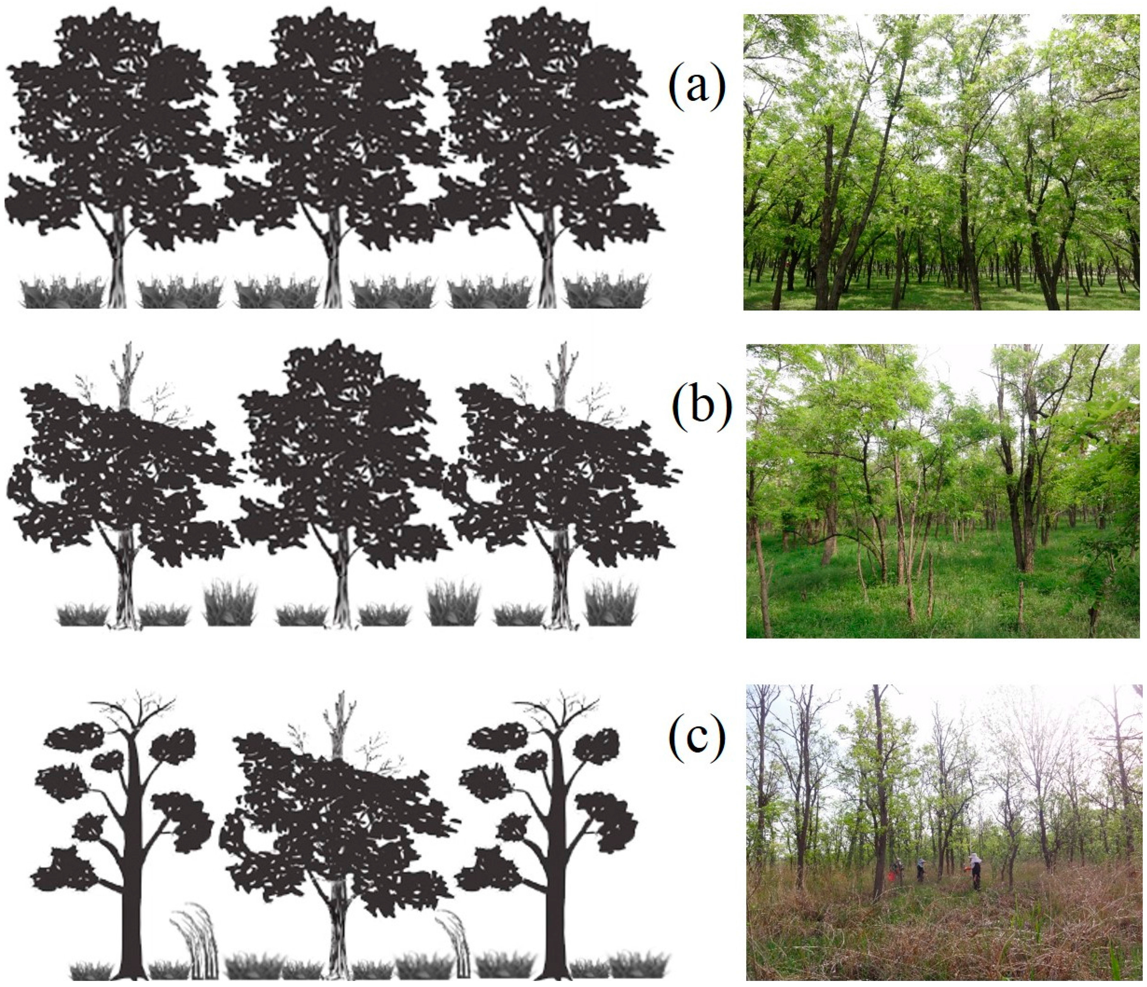
3.2. Crown Condition Classification Standard

Within each of the 375 subplots, three average Robinia pseudoacacia trees were selected and evaluated according to the USFS (United States Forest Service) Crown Condition Classification Guide (CCCG) standard [55]. These CCCG indicator data were then averaged from the five subplots for each plot and each indicator was classified into one class from the three vigor classes based on a range of values in the CCCG (see Table 1).

Table 1. The CCCG ^a tree vigor indicators and classification thresholds ^b.

Indicator	Healthy	Medium Dieback	Severe Dieback
Live crown ratio	>90%	70%–85%	50%–65%
Crown density	>80%	50%–70%	20%–40%
Crown diameter	>55%	26%–54%	1%–25%
Dieback	0%–5%	10%–25%	>30%
Foliar transparency	0%–20%	30%–50%	>60%

^a CCCG: Crown Condition Classification Guide; ^b Values of 100% were recorded as 99%, and intermediate values were upgraded to the next full 5% grouping.

Table 1. The CCCG ^a tree vigor indicators and classification thresholds ^b.

Indicator	Healthy	Medium Dieback	Severe Dieback
Live crown ratio	>90%	70%–85%	50%–65%
Crown density	>80%	50%–70%	20%–40%
Crown diameter	>55%	26%–54%	1%–25%
Dieback	0%–5%	10%–25%	>30%
Foliar transparency	0%–20%	30%–50%	>60%

^a CCCG: Crown Condition Classification Guide; ^b Values of 100% were recorded as 99%, and intermediate values were upgraded to the next full 5% grouping.

3.3. GLCM Textures and Local Spatial Statistics

3.3.1. The Grey-Level Co-Occurrence Matrix (GLCM)

GLCM was suggested as a mechanism for deriving texture measures [57]. Spatial co-occurrence texture analysis requires a user to identify five different control variables [29]: (1) window size; (2) the texture measure(s); (3) input channel (i.e., spectral channel to measure the texture); (4) quantization level of output channel (eight-bit, 16-bit, or 32-bit); and (5) the spatial component (i.e., the inter-pixel distance and angle during co-occurrence computation). Previous research on spruce forest structure variables (including age, top height, circumference, stand density, and basal area) using IKONOS imagery recommended the selection of textural features with consideration of the window size, the displacement, and direction [31]. We adopted this method to compute GLCM textures from IKONOS MS bands. The input pixel values were quantized to 32 discrete levels that led to a 32 × 32 element GLCM matrix. Given a large enough window size, any offset could be used, but (1, 1) is the most commonly used offset [58]. Therefore the displacement of (1, 1) was adopted. In this study we focused on three GLCM control variables, namely, the window size, the texture measure, and the direction based on IKONOS Band 4 (NIR band). The reasons for choosing Band 4 to test the effects of the window size and direction on classifying forest health conditions include (1) the workload was too heavy to test all window sizes and directions for all four MS bands; (2) per statistics of training samples of Robinia pseudoacacia health conditions extracted from MS bands (Figure 2), Band 4 was the most effective to discriminate among three health levels; and (3) Pu and Cheng [59] supported the fact that the TM NIR band was the most important to correlate with LAI (note that TM NIR band has the same wavelength as IKONOS Band 4). Thus the optimal window size and direction would be determined based on IKONOS Band 4, and then the determined window size and direction would be applied to all other IKONOS MS bands.

Figure 2. Means (bars) and standard deviations (short lines) of training samples of three health conditions of Robinia pseudoacacia extracted from IKONOS MS bands. Bands 1–4 represent IKONOS blue, green, red, and NIR band, respectively.

Figure 2. Means (bars) and standard deviations (short lines) of training samples of three health conditions of Robinia pseudoacacia extracted from IKONOS MS bands. Bands 1–4 represent IKONOS blue, green, red, and NIR band, respectively.

For this study, eight widely used GLCM features were selected (Table 2). Window size is an important component of a texture analysis because the texture is a multi-scale phenomenon [60]. If the window size is too small then it does not contain enough information about the area to perform an accurate analysis. However, if the window is too large, then it can overlap with other types of ground cover, and produces erroneous results. This is referred to as the edge effect [61,62]. In this study, we calculated eight GLCM features from IKONOS Band 4 starting from a 3 × 3 window size until an optimal window size leading to the highest classification accuracy could be identified. Since the directionality of texture has the potential to discriminate between isotropic and anisotropic structures [26], we also calculated eight GLCM measures from four directions (0°, 45°, 90°, 135°) based on IKONOS Band 4 to see whether the direction had any impact on the classification accuracy. Then the determined optimal window size and direction were applied to other IKONOS MS bands. Finally, 32 GLCM features (4 MS bands × 8 GLCM measures) extracted from the four MS bands based on the optimal window size and direction were used to classify Robinia pseudoacacia forests’ health conditions with an RF classifier. The GLCM textural analysis was implemented with the ENVI software [63].

3.3.2. Local Spatial Statistics

Spatial variations of forest health conditions were assessed across the study area through the Getis statistic (Gi). From an application perspective and in consideration of remote sensed imagery, pixels from a healthy tree crown will generate clusters that differ in intensity from pixel clusters from a dieback tree crown. The Gi [34], as a dimensionless indicator, expresses the sum of the weighted variable values p_i for some distance d of a particular unit cell i as a proportion of the sum of the variable values over the entire study area (Table 2). In this study, the Gi was used to analyze spatial autocorrelation characteristics of forest health conditions. Toward this objective, the Gi statistics or features were computed with a series of increasing distance value ranging from 1 pixel (i.e., window size of 3 × 3 pixels) and with seven neighborhood rules (including Rook’s case, Bishop’s case, Queen’s case, Horizontal, Vertical, Positive slope, and Negative slope) [34] from four IKONOS MS bands, respectively, using the ENVI software. This procedure was repeated with increasing lag sizes until the distance value leading to the highest classification accuracy could be identified. With this optimal distance value, we compared and selected an optimal neighborhood rule that could lead to the highest classification accuracy.

Table 2. A list of GLCM texture measures ^a and Gi statistic ^b, extracted from the four IKONOS MS bands and used in this analysis.

Name	Feature	Formula
GLCM Texture Measures
MEA (B#)	Mean	${\displaystyle \sum }_{i,j=0}^{N-1}ip\left(i,j\right)=u$
VAR (B#)	Variance	${\displaystyle \sum }_{i,j=0}^{N-1}p\left(i,j\right)\left(i-u\right)²$
HOM (B#)	Homogeneity	${\displaystyle \sum }_{i,j=0}^{N-1}\frac{p\left(i,j\right)}{1+{\left(i,j\right)}^2}$
CON (B#)	Contrast	${\displaystyle \sum }_{i,j=0}^{N-1}p\left(i,j\right)\left(i-j\right)²$
DIS (B#)	Dissimilarity	${\displaystyle \sum }_{i,j=0}^{N-1}p\left(i,j\right)\left|i-j\right|$
ENT (B#)	Entropy	${\displaystyle \sum }_{i,j=0}^{N-1}p\left(i,j\right)\left(-\ln p\left(i,j\right)\right)$
ASM (B#)	Angular Second Moment	${\displaystyle \sum }_{i,j=0}^{N-1}p\left(i,j\right)²$
COR (B#)	Correlation	${\displaystyle \sum }_{i,j=0}^{N-1}p\left(i,j\right)\frac{\left(i-u_i\right)\left(j-u_j\right)}{\sqrt{{\text{σ}}_i^2{\text{σ}}_j^2}}$
Gi Statistic
Gi (B#)	Getis statistic	$\frac{{{\displaystyle \sum }}_i^n{{\displaystyle \sum }}_j^n{w}_{ij}\left(d\right)p_i{p}_j}{{{\displaystyle \sum }}_i^n{{\displaystyle \sum }}_j^n{p}_i{p}_j}, j \ne i$

Note: (B#) represents the band number of IKONOS MS imagery. Per the GLCM texture measure, i, j are the row/column numbers in a spatial-dependence matrix; p (i, j) is the value in the cell i, j in the matrix; N is the number of rows or columns and equals to the number of grey levels. Per the Gi statistic, w_ij (d) is a symmetric one/zero spatial weight matrix with ones for all links defined as being within distance d of a given i; all other links are zero including the link of point i to itself; i is a given pixel and j are the pixels (not including the ith pixel) in the image, p_i, p_j are the pixel values; n is the total number of pixels in the image. ^a Haralick et al. [57]; ^b Getis and Ord [34].

Table 2. A list of GLCM texture measures ^a and Gi statistic ^b, extracted from the four IKONOS MS bands and used in this analysis.

Name	Feature	Formula
GLCM Texture Measures
MEA (B#)	Mean	${\displaystyle \sum }_{i,j=0}^{N-1}ip\left(i,j\right)=u$
VAR (B#)	Variance	${\displaystyle \sum }_{i,j=0}^{N-1}p\left(i,j\right)\left(i-u\right)²$
HOM (B#)	Homogeneity	${\displaystyle \sum }_{i,j=0}^{N-1}\frac{p\left(i,j\right)}{1+{\left(i,j\right)}^2}$
CON (B#)	Contrast	${\displaystyle \sum }_{i,j=0}^{N-1}p\left(i,j\right)\left(i-j\right)²$
DIS (B#)	Dissimilarity	${\displaystyle \sum }_{i,j=0}^{N-1}p\left(i,j\right)\left|i-j\right|$
ENT (B#)	Entropy	${\displaystyle \sum }_{i,j=0}^{N-1}p\left(i,j\right)\left(-\ln p\left(i,j\right)\right)$
ASM (B#)	Angular Second Moment	${\displaystyle \sum }_{i,j=0}^{N-1}p\left(i,j\right)²$
COR (B#)	Correlation	${\displaystyle \sum }_{i,j=0}^{N-1}p\left(i,j\right)\frac{\left(i-u_i\right)\left(j-u_j\right)}{\sqrt{{\text{σ}}_i^2{\text{σ}}_j^2}}$
Gi Statistic
Gi (B#)	Getis statistic	$\frac{{{\displaystyle \sum }}_i^n{{\displaystyle \sum }}_j^n{w}_{ij}\left(d\right)p_i{p}_j}{{{\displaystyle \sum }}_i^n{{\displaystyle \sum }}_j^n{p}_i{p}_j}, j \ne i$

Note: (B#) represents the band number of IKONOS MS imagery. Per the GLCM texture measure, i, j are the row/column numbers in a spatial-dependence matrix; p (i, j) is the value in the cell i, j in the matrix; N is the number of rows or columns and equals to the number of grey levels. Per the Gi statistic, w_ij (d) is a symmetric one/zero spatial weight matrix with ones for all links defined as being within distance d of a given i; all other links are zero including the link of point i to itself; i is a given pixel and j are the pixels (not including the ith pixel) in the image, p_i, p_j are the pixel values; n is the total number of pixels in the image. ^a Haralick et al. [57]; ^b Getis and Ord [34].

3.4. Random Forest Classification

Random forests [46] grow many regression trees without statistical pruning, and the result is based on the average of all the regression trees. Individual regression trees in the forest are built using bootstrap aggregation (bagging), which involves randomly drawing, with replacement, a bootstrap sample of the original training dataset. Each subset selected using bagging to make each individual tree grow usually contains two thirds of the calibration dataset. The samples that are not present in the calibration subset are included as part of another subset called out-of-bag (OOB). In addition to bagging, each tree split is based on a random subset of the input variables [46]. Therefore, the randomness introduced in the dataset selection and in the variable selection (mtry) makes random forests an accurate tool for prediction. Additionally, there are only two tuning parameters required for growing random forests, the number of trees to be grown (ntree), and the number of possible splitting variables (mtry) that are sampled at each node. In this study, we used the default values, i.e., mtry equals the number of root mean square of predictive variables and ntree = 500, as previous researchers have shown that sensitivity of the user-defined parameters is minimal and the default values are often a good choice [64,65].

A useful byproduct of RF is individual variable importance, which is a measure of the strength of a variable in the final model. RF variable importance is a useful output for gaining better insight into which variable or set of variables is the most relevant for the classification of the classes. To assess the importance of each feature, the RF switches one of the input random variables while keeping the rest constant, and it measures the decrease in accuracy that has taken place by means of the OOB error estimation and of Gini Index decrease [46]. We utilized the variable importance to rank the IKONOS spectral/textural/spatial features to account for their ability to discriminate amongst healthy, medium, and severe dieback Robinia pseudoacacia trees.

Although the RF algorithm does include a built-in “out-of-bag” validation scheme, previous study has proved OOB error was insufficient for spatial data [66]. Thus we used an independent validation data set to assess the RF classification accuracy. The ground reference dataset was randomly divided into two thirds (150 polygons) and one third (75 polygons) for training and validation, respectively. RF classification was performed using imageRF [67], which is a license-free platform that can be integrated into commercially-available IDL/ENVI software and can also be run as an add-on EnMAP-Box, which is an open-source and platform-independent software interface for image processing. In this study, confusion matrices were used to assess the classification accuracy from independent validation samples. Kappa index, overall accuracy (OA), Producer’s accuracy (PA), and User’s accuracy (UA) [68,69] were used to assess accuracies of classifying forest health conditions with different spectral/textural/spatial features.

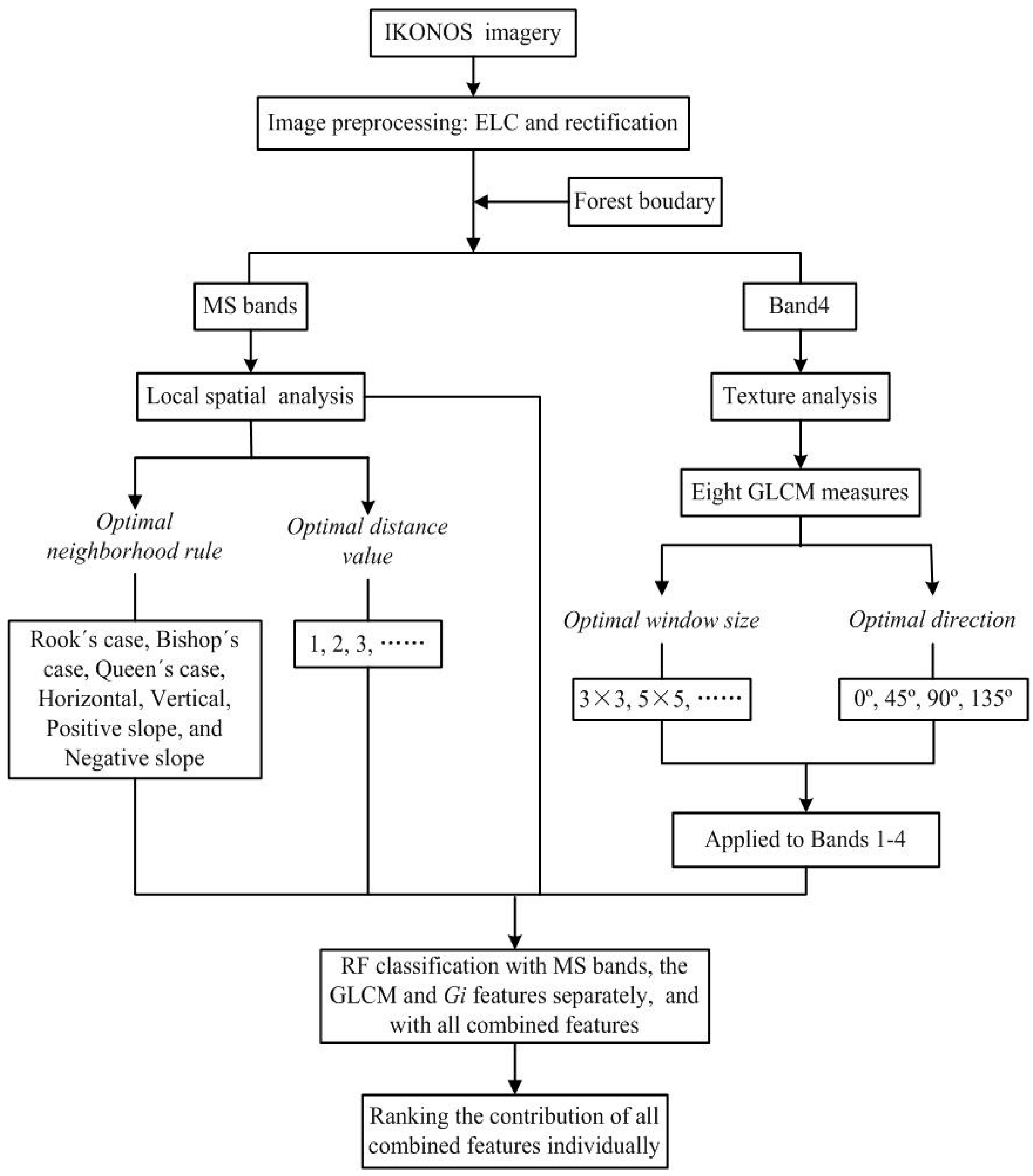
3.5. Experimental Procedure

In this study, the experimental procedure was carried out by using the ENVI software and imageRF software. Figure 3 presents a flowchart for forest health conditions classification using IKONOS MS bands, GLCM features, Gi features, and a combination of the three datasets. In this experiment, after IKONOS imagery data were preprocessed, the procedure of RF classification could be executed with the following four main steps:

(1)

classifying imagery using MS spectral bands only;

(2)

classifying imagery using the GLCM textural features only;

(3)

classifying imagery using the local spatial Gi features only; and

(4)

classifying imagery using combined MS bands, GLCM, and Gi features, and ranking the contribution of the spectral/textural/spatial features to the classification.

Figure 3. A flowchart of the analysis procedure for identifying and mapping the three health conditions of Robinia pseudoacacia. See the text for the full names of those abbreviations used in the figure.

Figure 3. A flowchart of the analysis procedure for identifying and mapping the three health conditions of Robinia pseudoacacia. See the text for the full names of those abbreviations used in the figure.

Step 1 was performed to provide a benchmark against which to compare with those using textural/spatial features only and using combinations of spectral, textural, and spatial features. The performance of the standard (benchmark) classification technique is necessary in order to measure whether incorporating textural/spatial information can improve classification accuracy.

At Step 2, the eight GLCM textures (Table 2) were first calculated from the IKONOS NIR band to determine the control variables (i.e., window size and direction) based on the highest RF classification accuracy, then the optimal window size and direction were applied to other MS bands, and finally GLCM features were used as input to run the RF classification. This step included: (1) calculating the eight GLCM measures from IKONOS Band 4 with window sizes from 3 × 3 through 17 × 17 and a fixed direction 135° to determine an optimal window size; (2) calculating the eight GLCM measures from IKONOS Band 4 with the optimal window size and four directions of 0°, 45°, 90°, and 135° to determine an optimal direction; (3) applying the optimal window size and direction to all four IKONOS MS bands to calculate 32 textures (8 GLCM measures × 4 MS bands); and (4) performing RF classifications using the eight GLCM textures calculated from Band 4 and all 32 GLCM textures calculated from the four MS bands.

At Step 3, first, an iterative classification scheme was used to determine the optimal distance value and the best neighborhood rule for calculating local spatial Gi features. Second, the four Gi features calculated with the optimum distance value and neighborhood rule from the four MS bands were used as input variables of the RF classifier.

At Step 4, the stack of MS bands, GLCM features and Gi features, determined at steps 2 and 3, was used as input to the RF classifier in order to explore whether a combination of MS+GLCM+Gi features could improve classification accuracy compared with using either MS bands, GLCM features, or Gi features only. Then all of the above predictive features were ranked to determine their differentiation ability in assessing Robinia pseudoacacia forest health conditions.

4. Results

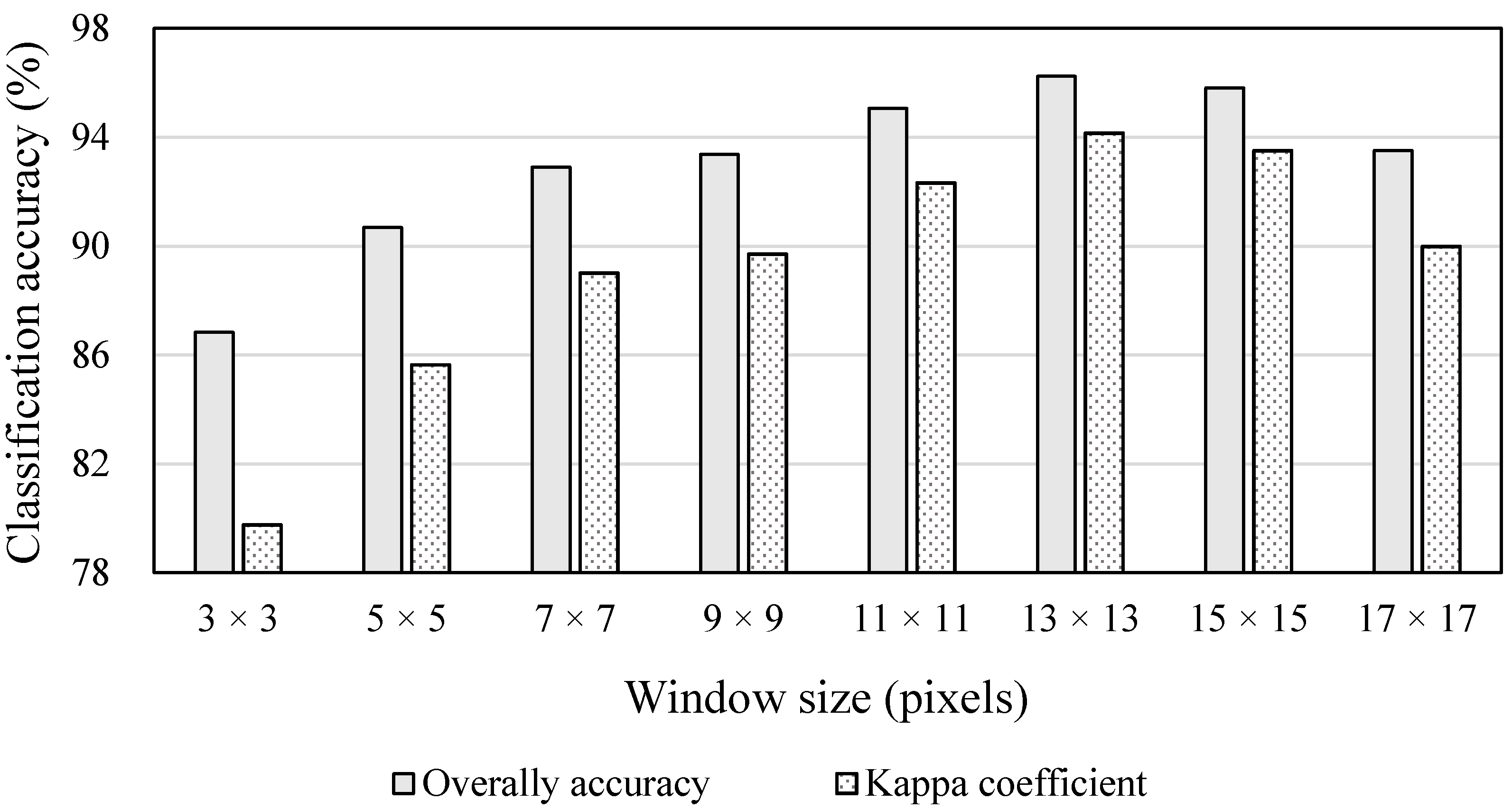
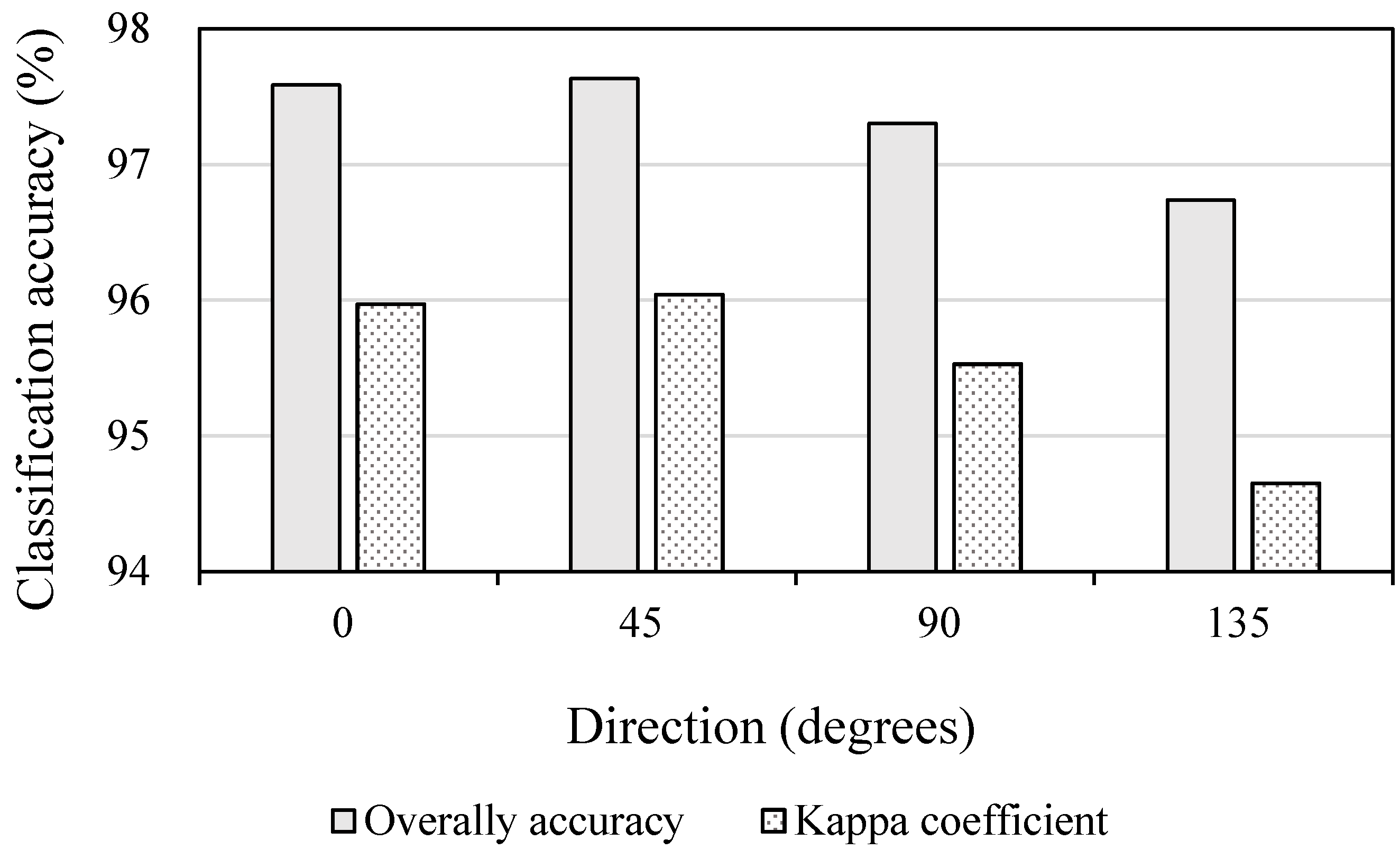
4.1. Determining the Optimal GLCM Window Size and Direction

Figure 4 shows how the classification accuracy changes as the window size increases from 3 × 3 to 17 × 17. All eight GLCM textural features from each window sizes were calculated from IKONOS Band 4 with direction 135°. From the figure, classification accuracy increases as the window size increases until the 13 × 13 window size. After that size, the OA and Kappa coefficients decrease slightly. Therefore, in this study, we chose the 13 × 13 window size as an optimal window size to compute the eight textural features to perform RF classification.

Next, with the fixed 13 × 13 window size, we further tested the effects of four directions (0°, 45°, 90°, 135°) on the RF classification result with the eight GLCM features extracted from IKONOS Band 4 (Figure 5). According to the OA, a direction of 45° has generated slightly better results compared to other directions. However, based on Producer’s accuracy differences among the four directions, calculated from the 13 × 13 window size for the three health levels, one-way ANOVA test (SPSS V.21.0, 2012) results indicated that the differences in producer’s accuracies among the four directions were not statistically significant at α = 0.05. Therefore a direction of 45° was selected as an “optimal” direction that may have a marginal accuracy and may be chosen just by chance. Moreover, the same one-way ANOVA test was also applied to three window sizes (from 11 × 11 to 15 × 15) with the fixed direction of 45°, and the test results also indicated that the differences of Producer’s accuracies among the three window sizes were not statistically significant at α = 0.05. Therefore the window 13 × 13 was selected as an “optimal” window size that may also have a marginal accuracy higher than that of the other window sizes. Finally the optimal determined window size of 13 × 13 and direction of 45° were applied to all four MS bands to extract a total of 32 GLCM features.

Figure 4. RF classification accuracies using the eight GLCM textural features across a range of window sizes. The eight GLCM texture measures were calculated from IKONOS Band 4 with a direction 135° and displacement 1 pixel.

Figure 4. RF classification accuracies using the eight GLCM textural features across a range of window sizes. The eight GLCM texture measures were calculated from IKONOS Band 4 with a direction 135° and displacement 1 pixel.

Figure 5. Comparison of overall accuracies of RF classification across four directions using the eight GLCM features calculated from IKONOS Band 4 with the window size of 13 × 13 and displacement 1 pixel.

Figure 5. Comparison of overall accuracies of RF classification across four directions using the eight GLCM features calculated from IKONOS Band 4 with the window size of 13 × 13 and displacement 1 pixel.

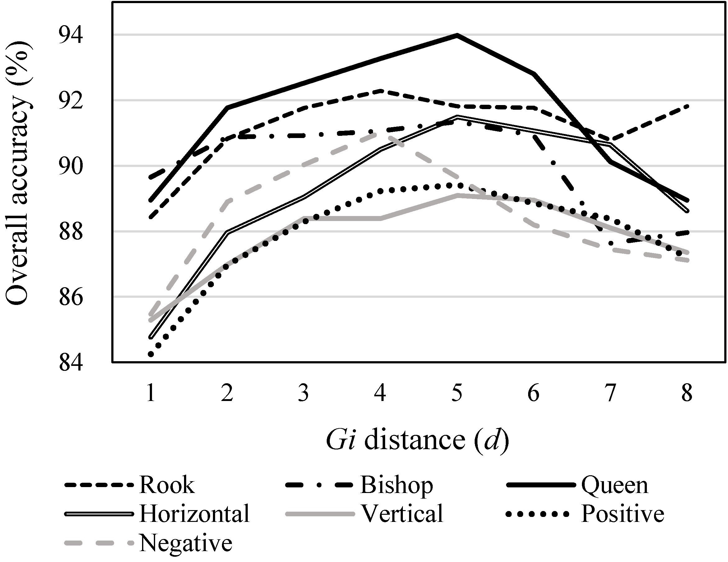
4.2. Determining the Optimal Gi Distance Value and Neighborhood Rule

When comparing results of classification using Gi features with varying distance values and neighborhood rules, it is easy to see from Figure 6 that the Queen’s neighborhood rule and the distance value of 5 would lead to the highest accuracy. Therefore, in this study, we adopted 5 as the optimal distance value and Queen’s as the optimal neighborhood rule to calculate the four Gi features from the four IKONOS MS bands for use in the RF classification.

Figure 6. Illustration of the effects of the Gi distance thresholds (unit: pixel) and neighborhood rules on the RF classification accuracies.

Figure 6. Illustration of the effects of the Gi distance thresholds (unit: pixel) and neighborhood rules on the RF classification accuracies.

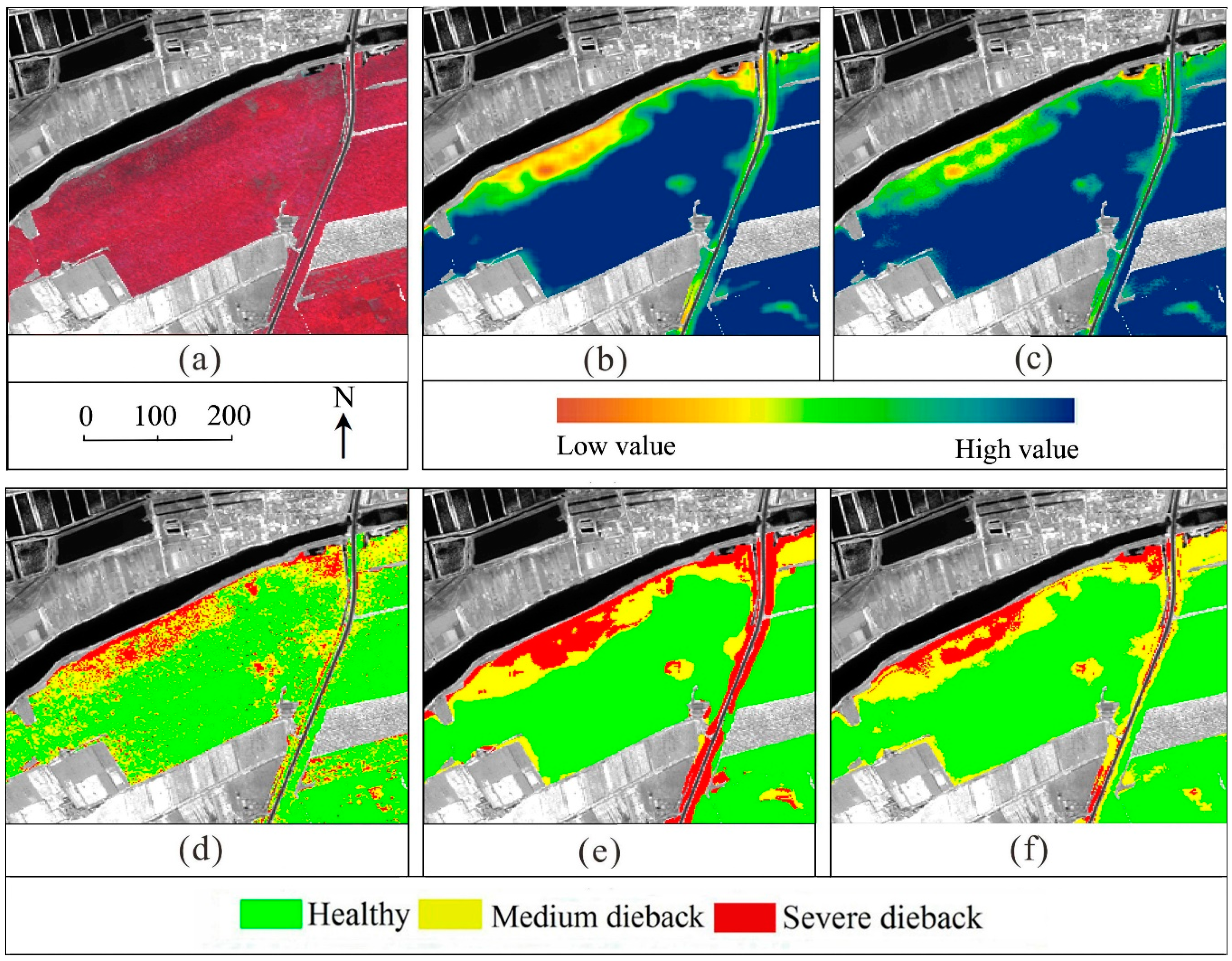
4.3. RF Classification Results

Table 3 lists the RF classification results based on a set of confusion matrices created with independent validation samples using spectral bands, textural features, spatial features, and spectral/textural/spatial features together. If only using spectral bands as input for RF classification, the OA was 79.5% and Kappa coefficient was 0.6821 with lower PA and UA for dieback forests (especially for medium dieback forest sites). If using the eight GLCM features calculated from IKONOS Band 4 as input, the OA of the forest health conditions classification was improved greatly to 97.1% compared to that created with the four MS bands only. However, if using all 32 GLCM features calculated from all four IKONOS MS bands as input, the OA of the forest health conditions classification decreased to 93.3%. The omission and commission errors for severe and medium dieback conditions of Robinia pseudoacacia forests, compared with those using the eight GLCM features as RF predictive variables, increased substantially. If using the four Gi features (calculated from the four MS bands) as input, the classification accuracy (94.0%) was almost the same as that using the 32 GLCM features as input (93.3%). The difference of accuracies between using these two datasets was that the commission errors for severe dieback and omission errors for medium dieback decreased substantially for the Gi features, while omission errors for healthy and commission errors for medium dieback increased slightly. In order to assess the performance of the combined features, the four MS bands, the eight GLCM features, and the four Gi features were combined and fed into the RF classifier. The reason we chose the eight GLCM features rather thanthe 32 GLCM features was that (1) the former yielded a higher classification accuracy and (2) the computational burden would be increased if we used all 32 GLCM features. Table 3 shows that the combined features (16) did not yield a higher classification accuracy (96.9%) than the GLCM features alone (eight) did (97.1%).

Table 3. Confusion matrices and RF classification accuracies using four spectral bands (reflectances); eight GLCM textures (calculated from Band 4 using the window size of 13 × 13 and direction 45°); 32 GLCM textures (calculated from the four MS bands using the window size of 13 × 13 and direction 45°); four Gi features (calculated from the four MS bands using distance value of 5 and Queen’s neighborhood rule); and four spectral, eight GLCM, and four Gi combined features together. The number in parentheses is the number of total features used. OA%: overall accuracy; PA%: Producer’s accuracy; UA%: User’s accuracy; M: medium; S: severe. Accuracy indices were computed based on independent validation samples.

	Spectral Features (4)		GLCM Features from Band 4 (8)		GLCM Features from 4 MS Bands (32)		Gi Features from 4 MS Bands (4)		All Combined Features (16)
OA	79.5		97.1		93.3		94.0		96.9
Kappa	0.7123		0.9554		0.8963		0.9065		0.9416
	PA	UA	PA	UA	PA	UA	PA	UA	PA	UA
Healthy	87.3	88.7	99.5	100.0	99.1	100.0	97.1	100.0	99.5	100.0
M dieback	69.9	67.3	98.1	93.2	92.5	87.0	97.3	85.5	98.4	92.4
S dieback	77.5	79.2	91.5	97.3	83.6	89.5	83.8	95.9	90.3	97.7

Table 3. Confusion matrices and RF classification accuracies using four spectral bands (reflectances); eight GLCM textures (calculated from Band 4 using the window size of 13 × 13 and direction 45°); 32 GLCM textures (calculated from the four MS bands using the window size of 13 × 13 and direction 45°); four Gi features (calculated from the four MS bands using distance value of 5 and Queen’s neighborhood rule); and four spectral, eight GLCM, and four Gi combined features together. The number in parentheses is the number of total features used. OA%: overall accuracy; PA%: Producer’s accuracy; UA%: User’s accuracy; M: medium; S: severe. Accuracy indices were computed based on independent validation samples.

	Spectral Features (4)		GLCM Features from Band 4 (8)		GLCM Features from 4 MS Bands (32)		Gi Features from 4 MS Bands (4)		All Combined Features (16)
OA	79.5		97.1		93.3		94.0		96.9
Kappa	0.7123		0.9554		0.8963		0.9065		0.9416
	PA	UA	PA	UA	PA	UA	PA	UA	PA	UA
Healthy	87.3	88.7	99.5	100.0	99.1	100.0	97.1	100.0	99.5	100.0
M dieback	69.9	67.3	98.1	93.2	92.5	87.0	97.3	85.5	98.4	92.4
S dieback	77.5	79.2	91.5	97.3	83.6	89.5	83.8	95.9	90.3	97.7

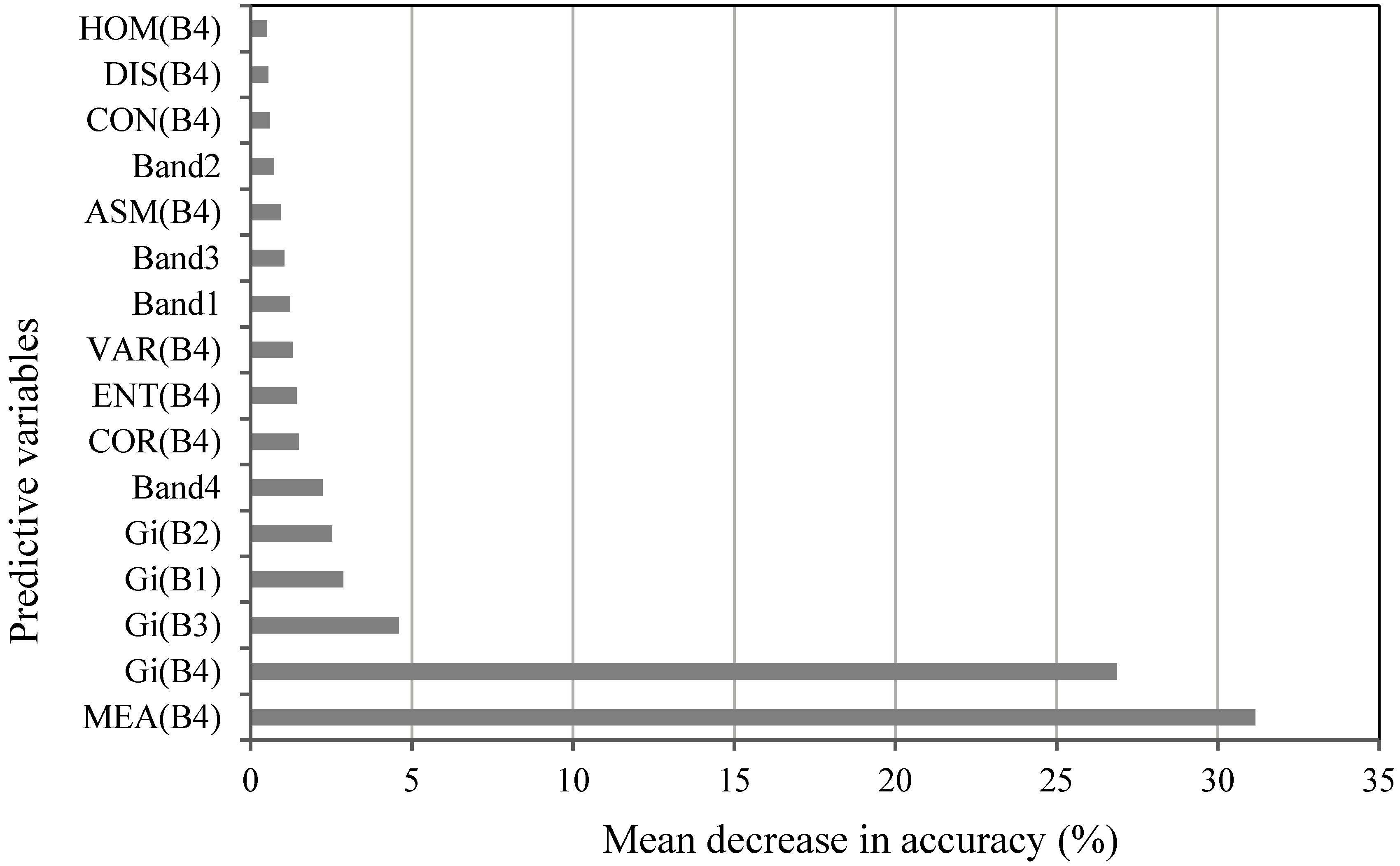
4.4. Contribution of All Predictive Variables

The combined features importance plot in Figure 7 presents the relative contributions of the 16 individual features for separating the three health conditions of Robinia pseudoacacia forests. The plot reveals that the most important predictive variable was GLCM texture mean, extracted from Band 4 of IKONOS imagery, followed by the Gi features calculated from Bands 4, 3, 1 and 2, and then Band 4. According to the accuracy values illustrated in Figure 7, the first and second ranked features MEA (B4) and Gi (B4) are 5–6 times more important than the third ranked feature (Gi (B3)).

5. Discussion

5.1. GLCM Feature Analysis

The moving window size of the GLCM is a key parameter in texture analysis. There are different methods for determining the window size for calculating textures. For example, Franklin et al. [70] used a range of experimental semivariograms to optimize the texture window size in remote sensing of forest inventory and forest structure characteristics. In this study, we determined the optimal window size by comparing RF classification accuracies. For the eight GLCM texture measures, the 13 × 13 window size was an ideal single window choice. Su et al. [71] found that GLCM angular secondary moment at a 45° angle could improve buildings classification using QuickBird image because buildings in Kuala Lumpur, Malaysia strike northwest and southeast, corresponding to the 135° direction. Kayitakire et al. [31] found that the direction parameter had minimal effects on retrieving forest structure variables in even-aged common spruce stands based on IKONOS-2 imagery. In our study area, the direction showed an insignificant impact on GLCM texture information. To compare the performance between textural and spatial features for classifying the three forest health levels, we computed the eight textural features from each IKONOS MS band. However, the eight GLCM features extracted from IKONOS Band 4 achieved a higher OA (97.1%) than that (93.3%) using all 32 GLCM features extracted from the four MS bands (Table 3). The reason for the lower classification accuracy created with the 32 GLCM features may be due to a large amount of redundant and inter-correlated textural information.

Figure 7. Combined individual features’ importance plot, expressed as the mean decrease in accuracy (%) when a feature was left out of a classification. B1, B2, B3, and B4 represent IKONOS blue band, green band, red band, and NIR band, respectively. The eight GLCM features were calculated from IKONOS Band 4 with the window size of 13 × 13 and direction 45°, and displacement 1 pixel. The Gi features were calculated from the four IKONOS MS bands with the distance value of 5 and Queen’s neighborhood rule.

Figure 7. Combined individual features’ importance plot, expressed as the mean decrease in accuracy (%) when a feature was left out of a classification. B1, B2, B3, and B4 represent IKONOS blue band, green band, red band, and NIR band, respectively. The eight GLCM features were calculated from IKONOS Band 4 with the window size of 13 × 13 and direction 45°, and displacement 1 pixel. The Gi features were calculated from the four IKONOS MS bands with the distance value of 5 and Queen’s neighborhood rule.

Figure 8b illustrates the GLCM MEA (B4) with the optimal window size of 13 × 13 and direction 45° covering a partial area of the study area. In this image, one can clearly distinguish many clusters of pixels of varying intensities. The majority of the imaging area was characterized by high GLCM Mean value (in blue in the image). Along the river channel in the north and along the road and drainage ditch from northeast to southwest, the values of MEA (B4) were smaller (in brown to yellow in the image).

5.2. Gi Feature Analysis

Ghimire et al. [39] found that making use of the Gi statistic with different distance values led to a substantial increase in per class classification accuracy of heterogeneous land-cover categories. The Kappa values of the RF classifications that used a combination of spectral and Gi variables at three different distance values (1, 3, and 5 pixels) ranged from 0.85 to 0.92 (vs. 0.78 using only spectral bands). In this study, we also compared classification accuracies at different distance values (from 1 to 8 pixels) and demonstrated that a distance value of 5 pixels was optimal (Figure 6). On the contrary, Myint et al. [38] reported that the Gi statistics calculated from IKONOS pan-sharpened MS bands using the shortest distance threshold (i.e., 1 pixel or 1 m) achieved the highest OA (75%) in urban land-use and land-cover classification. A small window size (or distance value) indicates that a spatial dependency is confined to a very localized region, while a large distance value indicates more spatially extensive spatial dependence [72]. Compared with heterogeneous urban areas, forest is relatively homogeneous, and thus the local spatial autocorrelation covers a larger area. In addition, the optimal distance value of 5 pixels (i.e., 11 × 11 window size for IKONOS MS bands) for Gi features was close to the optimal window size of 13 × 13 for GLCM features.

Figure 8. Comparison between (a) a subset of false color IKONOS composite image (NIR band/red band/green band vs. R/G/B); (b) GLCM texture MEA (B4) calculated from IKONOS NIR band with window size of 13 × 13 and direction 45°; (c) Gi (B4) calculated from IKONOS NIR band with distance value of 5 and the Queen’s neighborhood rule; (d) RF classification result created with the four IKONOS MS bands; (e) RF classification result created with the eight GLCM features calculated from IKONOS NIR band with the window size of 13 × 13 and direction 45°; and (f) RF classification result created with the four Gi features calculated from each IKONOS MS band with the distance value of 5 and Queen’s neighborhood rule.

Figure 8. Comparison between (a) a subset of false color IKONOS composite image (NIR band/red band/green band vs. R/G/B); (b) GLCM texture MEA (B4) calculated from IKONOS NIR band with window size of 13 × 13 and direction 45°; (c) Gi (B4) calculated from IKONOS NIR band with distance value of 5 and the Queen’s neighborhood rule; (d) RF classification result created with the four IKONOS MS bands; (e) RF classification result created with the eight GLCM features calculated from IKONOS NIR band with the window size of 13 × 13 and direction 45°; and (f) RF classification result created with the four Gi features calculated from each IKONOS MS band with the distance value of 5 and Queen’s neighborhood rule.

Figure 8c presents an example of an image created with Gi (B4). By visually comparing Figure 8c with GLCM Mean image in Figure 8b, we found that the spatial structure of the two images was very similar, with a larger area of low values along river channels and road lines.

Figure 7 shows that the first and second important features were both computed from IKONOS NIR band (Band 4). This is because, compared with other visible bands, (1) Band 4 is more effective for detecting healthy or diseased trees with reduced cell vigor (Figure 2) and (2) the NIR band has the greater penetration energy through the canopy, and thus the band, reflecting more understory and ground surface information, can characterize more subtle spatial variation than visible bands. A similar observation was reported by Treits and Hwarth [73].

5.3. Stability of the RF Variable Importance

A RF allows for assessment of the importance of the variables by means of the Gini index and the OOB subset [46]. Some researchers have reported that the stability of RF variable importance was dependent on the number of trees used in the ensemble (e.g., [46,74]), while other researchers have opted to calculate the variable importance after running the RF algorithm many times using different training subsamples of an original dataset [75]. In order to assess the stability of variable importance in this study, RF classification was performed with a different number of trees. We chose GLCM features (8) (Table 2) as an example of RF input with the number of trees from 100 to 800 with an interval of 100. The results demonstrated that the rank of variable importance was always the same with statistically insignificant (at α = 0.05 based on one-way ANOVA test result) change in the variable importance value.

5.4. Implications for Classification of Forest Health Conditions

Among the different spectral, textural, and spatial feature datasets, spectral-only data (i.e., four band reflectance) resulted in the lowest classification accuracy, with a serious salt-and-pepper phenomenon in the classification map (Figure 8d). This was especially obvious for medium or severe dieback forest stands with lower PA and UA in Table 3. Due to understory green grass showing a similar spectral appearance to the healthy tree canopy, it was difficult to distinguish between the healthy and dieback forest crowns using image spectral information only. On the contrary, GLCM features (eight)- and Gi features (four)-based classification accuracy improved greatly (Table 3). The commission and omission errors for the three health conditions of forest stands have substantially decreased (Table 3). This indicated that both textural and local spatial information in the Robinia pseudoacacia forests could help quantify the degree of spatial homogeneity or heterogeneity of different forest conditions. Figure 8e,f shows an almost similar clustered pattern in the classification map of forests’ health conditions using textural and spatial features separately.

In the study area, Robinia pseudoacacia forests are plantations with tree spacing ranging from 3 to 4 m with an average crown diameter of 4–6 m. Based on field survey data, we found that the crown closure was >80%, foliar transparency was <20% and crown diameter was >5.5 m in healthy forest stands with an understory of stunted and shade-tolerant grasses (such as Carex rigescens, Humulus scandens, etc.). In medium dieback forest stands, crown closure was between 50 and 70%, foliar transparency was between 30 and 50%, and crown diameter was between 4.5 and 5.5 m. The understory grass types changed and heliophytes (such as Viola philippica, Setaria viridis, etc.) appeared. With the continuous dieback tree crowns, the understory was covered by tall and dense grasses (such as Imperata cylindrical, Sonchus oleraceus, etc.) with the tree crown closure decreased to 20–40%, foliar transparency >60%, and crown diameter <4.5 m. When a severe dieback forest was near a river or lakeside, Phragmites australis was the predominant understory. Figure 9 shows the schematic representation of three conditions of forest plots. At healthy forest sites (Figure 9a), live tree crowns predominantly occupied each pixel within a window size of 13 × 13 image. Thus, for the homogeneous healthy forests, the image texture was relatively smooth and local spatial dependence was relatively high, leading to a high texture MEA (B4) and Gi (B4) value (blue color in Figure 8b,c). Inversely, at dieback forest sites (see Figure 9b,c), image pixels within the 13 × 13 window size might be covered by different components of dieback crown, live crown, understory grass, canopy shadow, or a mixture of the components, and thus the texture of dieback forest stand would be relatively rough with lower texture mean values (from yellow to brown color in Figure 8b). With the increase of tree dieback, which led to a higher local spatial variation, Gi (B4) values decreased correspondingly (from yellow to brown color in Figure 8c).

Figure 9. Schematic representation of three health conditions of forest plots, each with varying dieback and crown density: (a) a healthy forest; (b) a medium dieback forest; and (c) a severe dieback forest. To the right are photographs representing each health category.

Figure 9. Schematic representation of three health conditions of forest plots, each with varying dieback and crown density: (a) a healthy forest; (b) a medium dieback forest; and (c) a severe dieback forest. To the right are photographs representing each health category.

Remotely sensed data can convey information regarding the distribution, structure, and condition of forests. It was obvious from Figure 8e that most medium and severe dieback forests were distributed along the river channel and road line/drainage ditch. This clustered spatial pattern indicated some underlying physical or ecological processes. Liang and Hua [75] found that there were three main factors that affected the dieback of Robinia pseudoacacia trees in this study area: soil texture, soil salt content, and ground water levels. Loam soil is suitable for Robinia pseudoacacia trees because it has good permeability for air and root growth. If the water table is less than 1 m, Robinia pseudoacacia trees will suffer from high mortality due to root rotting and crown dieback because of long-time waterlogging. Robinia pseudoacacia trees can grow healthily with a soil salt content of less than 0.3%. In the YRD, soil salinity is related to ground elevation, groundwater depth, soil texture, and micro-geomorphology [76]. Zhang and Xing [77] found that higher soil salinity, lower nutrient content, and higher soil bulk density existed at dieback Robinia pseudoacacia forest stands in this study area. Thus inclusion of ancillary data (such as soil salt content, soil texture, groundwater levels, and micro-geomorphology type) in the RF classification may help our understanding of the mechanism of tree crown dieback and improve classification accuracy for future applications. Moreover, in addition to GLCM and Gi features, other spatial features such as morphological textural features [78], which have been proved promising in distinguishing red (Rhizophora mangle), white (Laguncularia racemosa), and black (Avicennia germinans) mangroves and rainforest regions with IKONOS imagery on the Caribbean coast of Panama, should be considered in future studies.

6. Conclusions

In this study we used spectral, spatial, and textural information extracted from IKONOS multispectral imagery and random forest (RF) classifier to determine three health conditions of Robinia pseudoacacia forests in the YRD, China. The experimental results demonstrated that both spatial and textural information outperformed spectral reflectance data. Nevertheless, the combination of all 16 features (four spectral, eight textural, and four spatial) did not yield better classification results than those created by the GLCM features alone (eight), which achieved the highest OA of 97.1%. In this study, to calculate the best local spatial statistical features, an optimal distance value of 5 pixels and the optimal Queen’s neighborhood rule were adopted. The best GLCM texture measures were calculated with the optimal window size of 13 × 13 and direction of 45°. RF variable importance proved that the IKONOS NIR band was the most effective for textural and spatial information extraction, leading to a high separability of Robinia pseudoacacia forests’ health conditions.

Our results also indicated that the RF classifier was a useful and robust tool for identification of forest health conditions using spectral, textural, and spatial features extracted from VHR remote sensing data as input. In addition, texture measures and local spatial statistics extracted from VHR imagery (e.g., IKONOS imagery in this study) could be used to characterize the spatial structure of stressed forests and help us better understand some underlying physical or ecological processes.

References

1. Raffa, K.F.; Aukema, B.H.; Bentz, B.J.; Carroll, A.L.; Hicke, J.A.; Turner, M.G.; Romme, W.H. Cross-scale drivers of natural disturbances prone to anthropogenic amplification: The dynamics of bark beetle eruptions. Bioscience 2008, 58, 501–517. [Google Scholar] [CrossRef]
2. Van Mantgem, P.J.; Stephenson, N.L.; Byrne, J.C.; Daniels, L.D.; Franklin, J.F.; Fulé, P.Z.; Harmon, M.E.; Larson, A.J.; Smith, J.M.; Taylor, A.H.; et al. Widespread increase of tree mortality rates in the western United States. Science 2009, 323, 521–524. [Google Scholar] [CrossRef] [PubMed]
3. Allen, C.D.; Macalady, A.K.; Chenchouni, H.; Bachelet, D.; McDowell, N.; Vennetierf, M.; Kitzbergerg, T.; Riglingh, A.; Breshearsi, D.D.; Hoggj, E.H.; et al. A global overview of drought and heat-induced tree mortality reveals emerging climate change risks of forests. For. Ecol. Manag. 2010, 259, 660–684. [Google Scholar] [CrossRef]
4. McDowell, N.; Pockman, W.T.; Allen, C.D.; Breshears, D.D.; Cobb, N.; Kolb, T.; Sperry, J.; West, A.; Williams, D.; Yepez, E.A. Mechanisms of plant survival and mortality during drought: Why do some plants survive while others succumb to drought? New Phytol. 2008, 178, 719–739. [Google Scholar] [CrossRef] [PubMed]
5. Manion, P.D. Tree Disease Concepts, 2nd ed.; Prentice-Hall Inc.: Upper Saddle River, NJ, USA, 1991; p. 416. [Google Scholar]
6. Manion, P.D.; Lachance, D. Forest Decline Concepts; APS Press: St. Paul, MN, USA, 1992; p. 249. [Google Scholar]
7. Haywood, A.; Stone, C. Mapping eucalypt forest susceptible to dieback associated with bell miners (Manorina melanophys) using laser scanning, SPOT 5 and ancillary topographical data. Ecol. Model. 2011, 222, 1174–1184. [Google Scholar] [CrossRef]
8. Rock, B.N.; Vogelmann, J.E.; Williams, D.L.; Vogelmann, A.F.; Hoshizaki, T. Remote detection of forest damage. BioScience 1986, 36, 439–445. [Google Scholar] [CrossRef]
9. Wulder, M.A.; Dymond, C.C.; White, J.C.; Leckie, D.G.; Carroll, A.L. Surveying mountain pine beetle damage of forests: A review of remote sensing opportunities. Forest Ecol. Manag. 2006, 221, 27–41. [Google Scholar] [CrossRef]
10. Breshears, D.D.; Cobb, N.S.; Rich, P.M.; Price, K.P.; Allen, C.D.; Balice, R.G.; Romme, W.H.; Kastens, J.H.; Floyd, M.L.; Belnap, J.; et al. Regional vegetation die-off in response to global-change-type drought. Proc. Natl. Acad. Sci. USA 2005, 102, 15144–15148. [Google Scholar] [CrossRef] [PubMed]
11. Dorigo, W.; Lucieer, A.; Podobnikar, T.; Čarni, A. Mapping invasive Fallopia japonica by combined spectral, spatial, and temporal analysis of digital orthophotos. Int. J. Appl. Earth Obs. Geoinf. 2012, 19, 185–195. [Google Scholar] [CrossRef]
12. Joria, P.E.; Ahearn, S.C. A comparison of the SPOT and Landsat Thematic Mapper satellite systems for detecting gypsy moth defoliation in Michigan. Photogramm. Eng. Remote Sens. 1991, 57, 1605–1612. [Google Scholar]
13. Royle, D.D.; Lathrop, R.G. Monitoring hemlock forest health in New Jersey using Landsat TM Data and change detection techniques. For. Sci. 1997, 43, 327–335. [Google Scholar]
14. Franklin, S.E.; Wulder, M.A.; Skakun, R.S.; Carroll, A.L. Mountain pine beetle red-attack forest damage classification using stratified Landsat TM data in British Columbia, Canada. Photogramm. Eng. Remote Sens. 2003, 69, 283–288. [Google Scholar] [CrossRef]
15. Wang, C.Z.; Lu, Z.Q.; Haithcoat, T.L. Using Landsat images to detect oak decline in the Mark Twain National Forest, Ozark Highlands. Forest Ecol. Manag. 2007, 240, 70–78. [Google Scholar] [CrossRef]
16. Coops, N.C.; Waring, R.H.; Wulder, M.A.; White, J.C. Prediction and assessment of bark beetle-induced mortality of lodgepole pine using estimates of stand vigour derived from remotely sensed data. Remote Sens. Environ. 2009, 113, 1058–1066. [Google Scholar] [CrossRef]
17. Negrón-Juárez, R.I.; Chambers, J.Q.; Guimaraes, G.; Zeng, H.; Raupp, C.F.M.; Marra, D.M.; Ribeiro, G.H.P.M.; Saatchi, S.S.; Nelson, B.W.; Higuchi, N. Widespread Amazon forest tree mortality from a single cross basin squall line event. Geophys. Res. Lett. 2010, 37, L16701. [Google Scholar] [CrossRef]
18. Ingram, J.C.; Dawson, T.P.; Whittaker, R.J. Mapping tropical forest structure in southeastern Madagascar using remote sensing and artificial neural networks. Remote Sens. Environ. 2005, 94, 491–507. [Google Scholar] [CrossRef]
19. Lee, S.H.; Cho, H.K. Detection of the pine trees damaged by pine wilt disease using high spatial remote sensing data. In Proceedings of the ISPRS Commission VII Symposium “Remote Sensing: From Pixels to Processes”, Enschede, The Netherlands, 8–11 May 2006.
20. Coops, N.C.; Johnson, M.; Wulder, M.A.; White, J.C. Assessment of QuickBird high spatial resolution imagery to detect red attack damage due to mountain pine beetle infestation. Remote Sens. Environ. 2006, 103, 67–80. [Google Scholar] [CrossRef]
21. Huang, X.; Zhang, L.; Li, P. An adaptive multiscale information fusion approach for feature extraction and classification of IKONOS multispectral imagery over urban areas. IEEE Geosci. Remote Sens. Lett. 2007, 4, 654–658. [Google Scholar] [CrossRef]
22. Radeloff, V.C.; Mladenoff, D.J.; Boyce, M.S. Detecting jack pine budworm defoliation using spectral mixture analysis: Separating effects from determinants. Remote Sens. Environ. 1999, 69, 156–169. [Google Scholar] [CrossRef]
23. Franklin, S.E.; Wulder, M.A.; Gerylo, G.R. Texture analysis of IKONOS panchromatic data for Douglas-fir forest age class separability in British Columbia. Int. J. Remote Sens. 2001, 22, 2627–2632. [Google Scholar] [CrossRef]
24. Gong, P.; Howarth, P. The use of structural information for improving land-cover classification accuracies at the rural-urban fringe. Photogramm. Eng. Remote Sens. 1990, 56, 67–73. [Google Scholar]
25. Huang, X.; Liu, X.; Zhang, L. A multichannel gray level co-occurrence matrix for multi/hyperspectral image texture representation. Remote Sens. 2014, 6, 8424–8445. [Google Scholar] [CrossRef]
26. Huang, X.; Zhang, L. An SVM ensemble approach combining spectral, structural, and semantic features for the classification of high-resolution remotely sensed imagery. IEEE Trans. Remote Sens. 2013, 51, 257–272. [Google Scholar] [CrossRef]
27. St-Onge, B.A.; Cavayas, F. Automated forest structure mapping from high resolution imagery based on directional semivariogram estimates. Remote Sens. Environ. 1997, 61, 82–95. [Google Scholar] [CrossRef]
28. Hsu, S.Y. Texture-tone analysis for automated land-use mapping. Photogramm. Eng. Remote Sens. 1978, 44, 1393–1404. [Google Scholar]
29. Franklin, S.; Maudie, A.; Lavlgne, M. Using spatial co-occurrence texture to increase forest structure and species composition classification accuracy. Photogramm. Eng. Remote Sens. 2001, 67, 849–855. [Google Scholar]
30. Lévesque, J.; King, D.J. Spatial analysis of radiometric fractions from high-resolution multispectral imagery for modelling individual tree crown and forest canopy structure and health. Remote Sens. Environ. 2003, 84, 589–602. [Google Scholar] [CrossRef]
31. Kayitakire, F.; Hamel, C.; Defourny, P. Retrieving forest structure variables based on image texture analysis and IKONOS-2 imagery. Remote Sens. Environ. 2006, 102, 390–401. [Google Scholar] [CrossRef]
32. Johansen, K.; Coops, N.C.; Gergel, S.E.; Stange, Y. Application of high spatial resolution satellite imagery for riparian and forest ecosystem classification. Remote Sens. Environ. 2007, 110, 29–44. [Google Scholar] [CrossRef]
33. Wang, H.; Pu, R.; Zhu, Q.; Ren, L.; Zhang, Z.Z. Mapping Health Levels of Robinia pseudoacacia Forests in the Yellow River Delta, China, Using IKONOS and Landsat 8 OLI Imagery. Int. J. Remote Sens. 2015, 36, 1114–1135. [Google Scholar]
34. Getis, A.; Ord, J.K. The analysis of spatial association by use of distance statistics. Geogr. Anal. 1992, 24, 189–206. [Google Scholar] [CrossRef]
35. Ord, J.K.; Getis, A. Local spatial autocorrelation statistics: Distributional issues and an application. Geogr. Anal. 1995, 27, 286–306. [Google Scholar] [CrossRef]
36. Anselin, L. Local indicators of spatial association-LISA. Geogr. Anal. 1995, 27, 93–115. [Google Scholar] [CrossRef]
37. Wulder, M.; Boots, B. Local spatial autocorrelation characteristics of Landsat TM imagery of managed forest area. Can. J. Remote Sens. 2001, 27, 67–75. [Google Scholar] [CrossRef]
38. Myint, S.W.; Wentz, E.A.; Purkis, S.J. Employing spatial metrics in urban land-use/land-cover mapping: Comparing the Getis and Geary indices. Photogramm. Eng. Remote Sens. 2007, 73, 1403–1415. [Google Scholar] [CrossRef]
39. Ghimire, B.; Rogan, J.; Miller, J. Contextual land-cover classification: Incorporating spatial dependence in land-cover classification models using random forests and the Getis statistic. Remote Sens. Lett. 2010, 1, 45–54. [Google Scholar] [CrossRef]
40. LeDrew, E.F.; Holden, H.; Wulder, M.A.; Derksen, C.; Newman, C. A spatial statistical operator applied to multidate satellite imagery for identification of coral reef stress. Remote Sens. Environ. 2004, 91, 271–279. [Google Scholar] [CrossRef]
41. Jin, Y.Q.; Yan, F. Monitoring sandstorms and desertification in northern China using SSM/I data and Getis statistics. Int. J. Remote Sens. 2004, 25, 2053–2060. [Google Scholar] [CrossRef]
42. Merzouki, A.; McNairn, H.; Pacheco, A. Mapping soil moisture using RADARSAT-2 data and local autocorrelation statistics. IEEE J. Sel. Top. App. Earth Obs. Remote Sens. 2011, 4, 128–137. [Google Scholar] [CrossRef]
43. Odongo, V.O.; Hamm, N.A.S.; Milton, E.J. Spatio-temporal assessment of Tuz Gölü, Turkey as a potential radiometric vicarious calibration site. Remote Sens. 2014, 6, 2494–2513. [Google Scholar] [CrossRef]
44. Goetz, S.J.; Wright, R.; Smith, A.J.; Zinecker, E.; Schaub, E. Ikonos imagery for resource management: Tree cover, impervious surfaces and riparian buffer analyses in the mid-Atlantic region. Remote Sens. Environ. 2003, 88, 195–208. [Google Scholar] [CrossRef]
45. Wulder, M.A.; Hall, R.J.; Coops, N.; Franklin, S. High spatial resolution remotely sensed data for ecosystem characterization. Bioscience 2004, 54, 511–521. [Google Scholar] [CrossRef]
46. Breiman, L. Random forests. Mach. Learn. 2001, 45, 5–32. [Google Scholar] [CrossRef]
47. Dye, M.; Mutanga, O.; Ismail, R. Combining spectral and textural remote sensing variables using random forests: Predicting the age of Pinus patula forests in KwaZulu-Natal, South Africa. J. Spat. Sci. 2012, 57, 193–211. [Google Scholar] [CrossRef]
48. Grinand, C.; Rakotomalala, F.; Gond, V.; Vaudry, R.; Bernoux, M.; Vieilledent, G. Estimating deforestation in tropical humid and dry forests in Madagascar from 2000 to 2010 using multi-date Landsat satellite images and the random forests classifier. Remote Sens. Environ. 2013, 139, 68–80. [Google Scholar] [CrossRef]
49. Abdel-Rahman, E.M.; Mutanga, O.; Adam, E.; Ismail, R. Detecting Sirex noctilio grey-attacked and lightning-struck pine trees using airborne hyperspectral data, random forest and support vector machines classifiers. ISPRS J. Photogramm. Remote Sens. 2014, 88, 48–59. [Google Scholar] [CrossRef]
50. Gislason, P.O.; Benediktsson, J.A.; Sveinsson, J.R. Random forests for land cover classification. Pattern Recognit. Lett. 2006, 27, 294–300. [Google Scholar] [CrossRef]
51. Cutler, D.R.; Edwards, T.C.; Beard, K.H.; Cutler, A.; Hess, K.T.; Gibson, J.; Lawler, J.J. Random forests for classification in ecology. Ecology 2007, 88, 2783–2792. [Google Scholar] [CrossRef] [PubMed]
52. Chan, J.C.W.; Paelinckx, D. Evaluation of Random forest and adaboost tree based ensemble classification and spectral band selection for ecotope mapping using airborne hyperspectral imagery. Remote Sens. Environ. 2008, 112, 2999–3011. [Google Scholar] [CrossRef]
53. Wulder, M.; Boots, B. Local spatial autocorrelation characteristics of remotely sensed imagery assessed with the Getis statistic. Int. J. Remote Sens. 1998, 19, 2223–2231. [Google Scholar] [CrossRef]
54. Xu, X.G.; Guo, H.H.; Chen, X.L.; Lin, H.P.; Du, Q.L. A multi-scale study on land use and land cover quality change: The case of the Yellow River Delta in China. GeoJournal 2002, 56, 177–183. [Google Scholar] [CrossRef]
55. Schomaker, M.E.; Zarnoch, S.J.; Bechtold, W.A.; Latelle, D.J.; Burkman, W.G.; Cox, S.M. Crown Condition Classification: A Guide to Data Collection and Analysis; Gen. Tech. Rep. SRS-102; U.S. Department of Agriculture, Forest Service, Southern Research Station: Asheville, NC, USA, 2007.
56. Jensen, J.R. Atmospheric correction. In Introductory Digital Image Processing: A Remote Sensing Perspective, 3rd ed.; Prentice Hall: Upper Saddle River, NJ, USA, 2005; pp. 210–213. [Google Scholar]
57. Haralick, R.M.; Shanmugan, K.; Dinstein, I. Texture features for image classification. IEEE Trans. Syst. Man Cyern. 1973, 3, 610–621. [Google Scholar] [CrossRef]
58. Hall-Beyer, M. GLCM Texture: A Tutorial, Version 2.10. Available online: http://www.fp.ucalgary.ca/mhallbey/tutorial.htm (accessed on 22 February 2015).
59. Pu, R.; Cheng, J. Mapping forest leaf area index using reflectance and textural information derived from WorldView-2 imagery in a mixed natural forest area in Florida, US. Int. J. Appl. Earth Obs. 2015, 42, 11–23. [Google Scholar] [CrossRef]
60. Moskal, L.M.; Franklin, S.E. Classifying multilayer forest structure and composition using high resolution, compact airborne spectrographic imager image texture. In Proceedings of the American Society of Remote Sensing and Photogrammetry Annual Conference, St. Louis, MO, USA, 23–27 April 2001.
61. Puissant, A.; Hirsch, J.; Weber, C. The utility of texture analysis to improve per pixel classification for high to very high spatial resolution imagery. Int. J. Remote Sens. 2005, 26, 733–745. [Google Scholar] [CrossRef]
62. Aplin, P. On scales and dynamics in observing the environment. Int. J. Remote Sens. 2006, 27, 2123–2140. [Google Scholar] [CrossRef]
63. ITTVIS. ITT Visual Information Solutions-Data Analysis and Visualization Software, Training and Consulting. February 2009. Available online: http://www.ittvis.com (accessed on 16 February 2009).
64. Lawrence, R.L.; Wood, S.D.; Sheley, R.L. Mapping invasive plants using hyperspectral imagery and Breiman Cutler classifications (Random Forest). Remote Sens. Environ. 2006, 100, 356–362. [Google Scholar] [CrossRef]
65. Ismail, R.; Mutanga, O. A comparison of regression tree ensembles: Predicating Sirex noctilio induced water stress in Pinus patula forest of KwaZulu-Natal, South Africa. Int. J. Appl. Earth Obs. Geoinf. 2010, 12, 45–51. [Google Scholar] [CrossRef]
66. Mascaro, J.; Asner, G.P.; Knapp, D.E.; Kennedy-Bowdoin, T.; Martin, R.E.; Anderson, C.; Higgins, M.; Chadwick, K.D. A tale of two “Forests”: Random forest machine learning aids tropical forest carbon mapping. PLoS One 2014, 9, e85993. [Google Scholar]
67. Waske, B.; van der Linden, S.; Oldenburg, C.; Jakimow, B.; Rabe, A.; Hostert, P. imageRF—A user-oriented implementation for remote sensing image analysis with Random Forests. Environ. Model. Softw. 2012, 35, 192–193. [Google Scholar] [CrossRef]
68. Congalton, R.G.; Mead, R.A. A quantitative method to test for consistency and correctness in photointerpretation. Photogramm. Eng. Remote Sens. 1983, 49, 69–74. [Google Scholar]
69. Story, M.; Congalton, R.G. Accuracy assessment—A user’s perspective. Photogramm. Eng. Remote Sens. 1986, 52, 397–399. [Google Scholar]
70. Franklin, S.; Wulder, M.; Lavigne, M. Automated derivation of geographic window sizes for use in remote sensing digital image texture analysis. Comput. Geosci. 1996, 22, 665–673. [Google Scholar] [CrossRef]
71. Su, W.; Li, J.; Chen, Y.; Liu, Z.; Zhang, J.; Low, T.M.; Suppiah, I.; Hashim, S.A.M. Textural and local spatial statistics for the object-oriented classification of urban areas using high resolution imagery. Int. J. Remote Sens. 2008, 29, 3105–3117. [Google Scholar] [CrossRef]
72. Griffith, P.; Getis, A.; Griffin, E. Regional patterns of affirmative action compliance costs. Ann. Reg. Sci. 1996, 30, 321–340. [Google Scholar] [CrossRef]
73. Treits, P.; Hwarth, P. High spatial resolution remote sensing data for forest ecosystem classification: An examination of spatial scale. Remote Sens. Environ. 2000, 76, 268–289. [Google Scholar] [CrossRef]
74. Rodriguez-Galiano, V.F.; Ghimire, B.; Rogan, J.; Chica-Olmo, M.; Rigol-Sanchez, J.P. An assessment of the effectiveness of a random forest classifier for land-cover classification. ISPRS J. Photogramm. Remote Sens. 2012, 67, 93–104. [Google Scholar] [CrossRef]
75. Liang, Y.; Long, Z. Theory and Technology on Robinia Pseudoacacia Cultivation; China Forestry Publishing: Beijing, China, 2010. [Google Scholar]
76. Zhang, J.; Xing, S. Research on soil degradation of Robinia pseudoacacia plantation under environmental stress. Chin. J. Soil Sci. 2009, 40, 1086–1091. [Google Scholar]
77. Wang, H.; Gong, P.; Liu, G. Multi-scale spatial variations in soil salt in the Yellow River Delta. Geogr. Res. 2006, 25, 649–658. [Google Scholar]
78. Huang, X.; Zhang, L.; Wang, L. Evaluation of morphological texture features for mangrove forest mapping and species discrimination using multispectral IKONOS Imagery. IEEE Geosci. Remote Sens. Lett. 2009, 6, 393–397. [Google Scholar] [CrossRef]