Prediction of Macronutrients at the Canopy Level Using Spaceborne Imaging Spectroscopy and LiDAR Data in a Mixedwood Boreal Forest

Abstract

Information on foliar macronutrients is required in order to understand plant physiological and ecosystem processes such as photosynthesis, nutrient cycling, respiration and cell wall formation. The ability to measure, model and map foliar macronutrients (nitrogen (N), phosphorus (P), potassium (K), calcium (Ca) and magnesium (Mg)) at the forest canopy level provides information on the spatial patterns of ecosystem processes (e.g., carbon exchange) and provides insight on forest condition and stress. Imaging spectroscopy (IS) has been used particularly for modeling N, using airborne and satellite imagery mostly in temperate and tropical forests. However, there has been very little research conducted at these scales to model P, K, Ca, and Mg and few studies have focused on boreal forests. We report results of a study of macronutrient modeling using spaceborne IS and airborne light detection and ranging (LiDAR) data for a mixedwood boreal forest canopy in northern Ontario, Canada. Models incorporating Hyperion data explained approximately 90% of the variation in canopy concentrations of N, P, and Mg; whereas the inclusion of LiDAR data significantly improved the prediction of canopy concentration of Ca (R² = 0.80). The combined used of IS and LiDAR data significantly improved the prediction accuracy of canopy Ca and K concentration but decreased the prediction accuracy of canopy P concentration. The results indicate that the variability of macronutrient concentration due to interspecific and functional type differences at the site provides the basis for the relationship observed between the remote sensing measurements (i.e., IS and LiDAR) and macronutrient concentration. Crown closure and canopy height are the structural metrics that establish the connection between macronutrient concentration and IS and LiDAR data, respectively. The spatial distribution of macronutrient concentration at the canopy scale mimics functional type distribution at the site. The ability to predict canopy N, P, K, Ca and Mg in this study using only IS, only LiDAR or their combination demonstrates the excellent potential for mapping these macronutrients at canopy scales across larger geographic areas into the next decade with the launch of new IS satellite missions and by using spaceborne LiDAR data.

1. Introduction

Macronutrients (nitrogen (N), phosphorus (P), potassium (K), calcium (Ca) and magnesium (Mg)) are required for plant physiological and ecosystem processes. For example, N is an important constituent of the chlorophyll molecule and the carbon-fixing enzyme ribulose-1, 5-bis-phosphate carboxylase/oxygenase and is thus directly related to photosynthesis [1]. Foliar N is also related to primary production and decomposition [2,3]. P is a component of nucleic acids, lipid membranes, sugar phosphates and ATP, which all have important roles in photosynthesis and respiration [1]. N and P are the major growth-limiting nutrients for plants worldwide [4]. Mg, like N, is also a constituent of the chlorophyll molecule and is directly related to photosynthesis [1]. K has a number of important roles in photosynthesis and respiration, including translocation of photosynthates into sink organs, maintenance of turgor pressure, activation of enzymes, N metabolism and reducing excess uptake of ions such as Na and Fe in saline and flooded soils [5,6]. Ca is required for cell division and cell wall synthesis, and light stimulates its uptake into chloroplasts where it is critical to the function of photosystem I [1,7].

The ability to measure, model and map foliar macronutrients at the canopy level allows us to examine these as proxies for assessing forest condition and stress, as well as ecosystem processes such as forest nutrient cycling and carbon (C) exchange (photosynthesis and net primary production (NPP)). Photosynthesis and NPP are of critical interest for the assessment of C fixation where forests function as sinks for C in the biosphere, given that global atmospheric carbon dioxide concentrations have been increasing at accelerating rates over the last several decades [8]. Macronutrients, in particular N, have been used as proxies for C exchange, or as parameters in ecosystem models. For example, canopy N concentration was used to estimate the NPP of temperate forest ecosystems coupled with field measurements and IS data by Smith et al. [3] and as a parameter in the PnET-II forest process model [9]. Thus, spatially-explicit landscape and regional inputs of foliar N concentration have the potential to improve the accuracy of ecosystem models.

A substantial portion of the published work regarding the prediction of nutrients at the canopy scale has focused on N. Although most canopy level studies have been conducted using airborne IS data, a few have examined satellite IS data. For example, Coops et al. [10] examined the utility of Hyperion IS data to predict N in eucalyptus forest canopies while Smith et al. [11] and Townsend et al. [12] compared the effectiveness of AVIRIS and Hyperion IS data to predict N concentration in temperate forest canopies. Canopy scale analysis to predict N from airborne IS data has been conducted in temperate [13,14,15,16] and tropical [17,18,19,20] forest ecosystems. Work in the boreal forest has been more limited. Ollinger et al. [21] and Knyazikhin et al. [22] did include a boreal coniferous forest site (i.e., Howland Forest, ME) in their studies examining N concentration across multiple ecosystems in the US, but more work is clearly needed in this biome.

Research examining the detection of P, K, Mg and Ca using IS data also has been more limited. The majority of studies have utilized field spectroradiometers to predict P in agricultural fields [23,24] and P and K in the foliage of giant sequoia and eucalyptus trees [25,26]. P, K, Mg and Ca concentrations have been examined in savannah grasses [27] as well as for willow, olive, grass and heather foliage [28]. At airborne scales, AVIRIS data were used to estimate area-integrated P concentrations in tropical forests of Hawaii [29] and African savannah using HyMap data [30]. Mirik et al. [31] found a statistically significant relationship between a simple ratio vegetation reflectivity index (1129 nm/469 nm) and P concentration on an area basis in the forage vegetation of Yellowstone National Park using PROBE-1 data. The small number of studies demonstrates that there is a clear need to investigate the utility of IS data for the estimation of P, K, Mg and Ca in forest canopies. To our knowledge, there is no study that investigates the utility of spaceborne IS data for the prediction of these macronutrients; hence there is a need to test the performance of spaceborne IS data for predicting these macronutrients at the canopy level. This is of interest to the scientific community because of the upcoming IS satellite missions such as the Hyperspectral Infrared Imager (HyspIRI) and the Environmental Mapping and Analysis Program (EnMAP), which will provide continuous global coverage with high fidelity IS data [32,33].

Conventionally, prediction of foliar chemicals using IS data has relied on the presence of absorption features associated with chemical constituents (e.g., pigments, N, cellulose, lignin, proteins) and water along the electromagnetic spectrum [34]. However, foliar biochemical estimation at the canopy level is plagued with several challenges. First, reflectance is attenuated and absorption features are masked due to presence of water in fresh foliage especially in the shortwave infrared (SWIR) [35]. Second, interior air-cell interfaces of fresh foliage randomly scatter light, which interferes with the signal from the subtle absorption features [36]. Third, reflectance data collected over vegetation canopies from airborne and spaceborne platforms are contaminated because of absorption and scattering of the atmosphere as radiation travels through it. Fourth, signal-to-noise ratios (SNR) for current spaceborne IS sensors is low. Fifth, the recorded signal is a mixture of background reflectance composed of soil, water and/or other cover types in environments with incomplete canopy cover. As a result, the spectral response of the vegetation canopy is a combination of the interactions between radiation and canopy structure (e.g., leaf area index, foliage clumping and orientation), atmosphere, background reflectance, sun-target-sensor geometry and absorption features associated with foliar chemicals, which constitute only a small fraction of the spectral response [22,37,38]. Therefore, it is difficult to relate and clearly identify mechanisms linking spectral data, in particular spaceborne spectral data, to nutrient concentration at the canopy level.

Progress has been made to address some of these problems. For example, atmospheric correction algorithms significantly reduce the impact of absorption and scattering. Transformations of the spectrum such as taking the first and second derivatives have been proposed to account for illumination and background effects [39,40]. Continuum removal was developed to enhance the absorption features along the spectrum by Kokaly and Clark (1999). This method has been used to estimate foliar chemical concentrations using spectra collected in the laboratory, field and from the canopy using airborne sensors [30,41,42,43].

Partial least squares (PLS) regression has become a commonly used method to relate IS data to foliar chemistry. PLS regression reduces the full spectrum to a smaller number of independent factors and takes into account the covariance between the response variable and the predictor variables during the dimensionality reduction process, which makes it superior to other methods like principal components analysis, which only takes into account the variance in the predictor variables [44,45]. This reduction process also helps avoid the problem of overfitting due to the presence of many more predictor variables (wavelengths) than dependent variables (chemical concentration), which is the case with IS data. In addition, it allows the full spectrum available after preprocessing to be utilized as opposed to specific bands or spectral regions to estimate chemical concentration. PLS regression has been used with IS data to estimate biochemical concentrations in plant canopies [18,46,47].

The species composition and deciduous and coniferous forest types, i.e., functional types, of the mixedwood boreal forest may provide an indirect method to model macronutrients at the canopy scale. Species composition exerts a major control on spatial patterns of foliar and canopy chemistry and has been shown across tropical, Mediterranean and temperate forests [18,46,48,49,50]. The mechanism that links species composition and canopy chemistry is based on the concept of the ‘global leaf economics spectrum’ [51]; i.e., plant traits that control key chemical, structural and physiological properties such as leaf mass per area (LMA), specific leaf area, leaf lifespan, photosynthesis, leaf N and P fall onto a spectrum across plant species, and species globally converge towards these functional traits [51,52]. With particular reference to K, Ca and Mg, 55% to 66% of the variation in their concentrations were accounted for by species in lowland Bornean forests [50] and approximately, 23%, 50% and 47% and 45%, 70% and 71% of the variance their concentrations were explained by species on lower fertility and higher fertility soils in the western Amazonian forests, respectively [53]. This is also likely to be the case in the mixedwood boreal forest, which contains deciduous and coniferous species and forest types. The canopy N:P ratio has been predicted and mapped based on the spatial variation generated by deciduous and coniferous forest types in a mixedwood boreal forest of northern Ontario [54].

LiDAR data have been used extensively to study boreal forest structure and physiology [55,56,57,58,59] as well as species identification [60]. The mixedwood boreal forest is structurally complex because the coniferous and deciduous species have different heights and canopy shapes. LiDAR can characterize this structural complexity since it provides information about the vertical and horizontal structure of the canopy [61]. If a covariate that establishes a link between the macronutrient concentration and LiDAR data can be identified, then it would be possible to predict macronutrients using LiDAR data. For example, crown closure was identified as the canopy structural metric that made it possible to relate LiDAR data to canopy N:P ratio in the mixedwood boreal forest [54].

Given the importance of species and forest types in controlling forest structure and foliar/canopy chemistry, we hypothesize that canopy macronutrient concentrations for a mixedwood boreal forest in northern Ontario can be modeled using IS and LiDAR data. To test this hypothesis, we examine spaceborne IS and airborne LiDAR data. Our objectives are: (i) to evaluate the utility of spaceborne IS data to estimate canopy macronutrient (N, P, K, Ca and Mg) concentrations; and (ii) to determine the potential for LiDAR data to improve the estimation of canopy nutrients by incorporating canopy structural information.

2. Materials and Methods

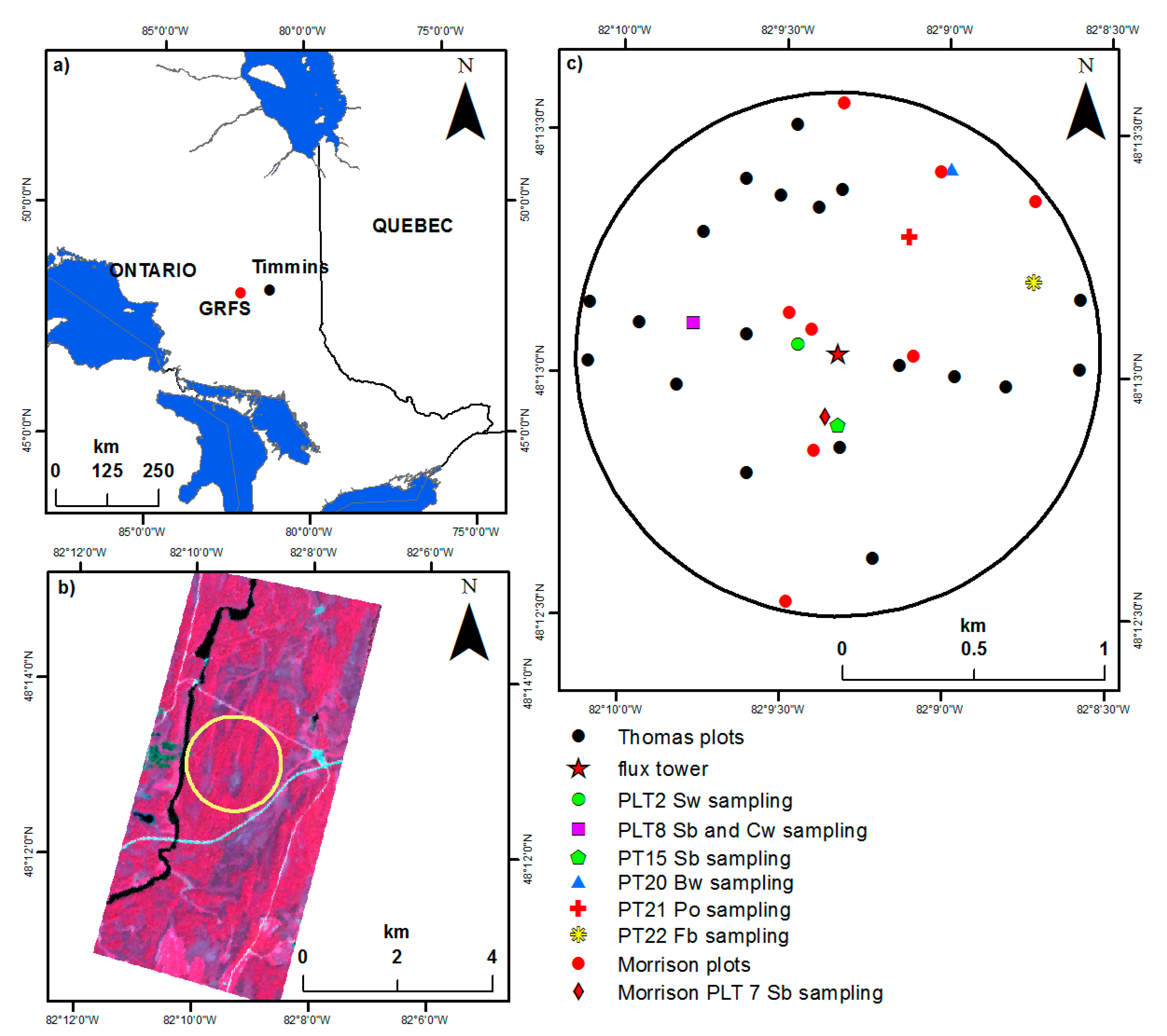
2.1. Study Site

This research was conducted at the mature mixedwood site at the Groundhog River Flux Station (GRFS); one of the stations of the Canadian Carbon Program (formerly the Fluxnet-Canada Research Network). The site is located approximately 80 km southwest of Timmins, Ontario, Canada (Figure 1a). A flux tower, 41 m tall with a 1 km footprint, is located at the site (Figure 1b,c). The site is representative of a mature boreal mixedwood forest with a patchy mixture of five primary tree species including trembling aspen (Po-Populus tremuloides Michx.), white birch (Bw-Betula papyrifera Marsh.), white spruce (Sw-Picea glauca [Moench] Voss), black spruce (Sb-Picea mariana [Mill.] B.S.P.), balsam fir (Fb-Abies balsamea [L.] Mill.), and distinct patches of northern white cedar (Cw-Thuja occidentalis [L.]). A total of 34 circular plots (11.3 m radius) were established using a stratified sampling scheme within the 1 km radius of the tower to capture the major species associations (Figure 1c). Field and remote sensing data used in this study were collected as part of the Canadian Carbon Program and the remote sensing and forest mensuration data have been used in previous studies [54,55,62].

2.2. Field Data

Multiple foliage samples were collected from the upper sunlit portions of the canopy from five trees in each of six different sampling plots for all species except black spruce for which 13 trees were sampled in July 2005 (Figure 1c). The number of leaves collected from each tree ranged from 10 to 40 leaves for deciduous species, and 400–1500 needles for coniferous species. Samples were analyzed at the inorganic laboratory of the Ontario Forest Research Institute (Sault Ste. Marie, Ontario) to determine the foliar concentration of N, P, K, Ca and Mg. Total N in the foliage was determined through the conversion of all forms of N into N₂ by dry combustion. The Kjeldahl method was used to extract the cations of P, K, Ca and Mg, which were measured using inductively coupled plasma-atomic emission spectroscopy. Average nutrient concentration for each species was calculated by averaging the results of the foliage samples. To scale the macronutrient concentration from leaf level to canopy level in each plot, the average nutrient concentration of a given species was multiplied by its species presence weighted by its biomass according to the formula below:

$$avg.nut plot={\displaystyle \sum }_{i=1}^n\left(avg.nu{t}_i\right)f_i$$

(1)

where i represents a given species in plot, avg.nut_i represents the average nutrient concentration for species i, and f_i is the biomass fraction of species i within the plot which is calculated by dividing the total biomass of species i by the total biomass of all species within the plot.

Figure 1. (a) Location of the Groundhog River Flux Station (GRFS). (b) Flux tower footprint at the mixedwood forest at the GRFS. (c) Plot layout and sample plot locations at the mixedwood forest site. Sw = white spruce (Picea glauca); Cw = northern white cedar (Thuja occidentalis); Sb = black spruce (Picea mariana); Bw = white birch (Betula papyrifera); Po = trembling aspen (Populus tremuloides); Fb = balsam fir (Abies balsamea).

Figure 1. (a) Location of the Groundhog River Flux Station (GRFS). (b) Flux tower footprint at the mixedwood forest at the GRFS. (c) Plot layout and sample plot locations at the mixedwood forest site. Sw = white spruce (Picea glauca); Cw = northern white cedar (Thuja occidentalis); Sb = black spruce (Picea mariana); Bw = white birch (Betula papyrifera); Po = trembling aspen (Populus tremuloides); Fb = balsam fir (Abies balsamea).

Forest mensuration data were collected in 2003 and 2004 in accordance with Fluxnet-Canada protocols [63] (now known as the Canadian Carbon Program). Diameter at breast height (dbh), height to the top of the crown, crown width taken along two axes assuming an elliptical shape, and species were recorded for each tree with a dbh greater than 9 cm within each plot. Structural metrics describing canopy shape including crown closure (percentage of ground covered by tree crowns as viewed from above) and height including average height (arithmetic mean of all tree heights), dominant height (maximum tree height), mean dominant height (mean height of the 100 largest trees ha⁻¹), Lorey’s height (tree height weighted by basal area) and basal area were calculated for each plot from these measurements. Total aboveground biomass (kg·ha⁻¹) for each plot was calculated summing the aboveground biomass of trees in the plot using the allometric equations developed for Ontario hardwoods and softwoods that incorporated dbh and tree height [64,65].

2.3. Remote Sensing Data

Hyperion EO-1 data (400–2500 nm with 10 nm spectral resolution and 30 m spatial resolution) were collected for the GRFS in July 2005 to coincide with the foliar sample collection. Hyperion data have a lower SNR than airborne sensors; hence, they require significant preprocessing. First, bands that had no data or had very low SNR were omitted from the analysis (149 spectral bands across 477–1346, 1487–1790 and 2032–2335 nm range were suitable for analysis). Second, scan lines that caused image striping were restored by taking the average of the adjacent lines. Subsequently, the data were atmospherically corrected using the fast line-of-sight atmospheric analysis of spectral hypercubes (FLAASH) program. FLAASH uses the MODTRAN4 radiation transfer code to convert radiance at the top of the atmosphere to reflectance at the surface pixel by pixel. Following atmospheric correction, geometric correction was completed using a 0.5 m resolution digital elevation model (DEM) generated from high-density (3–8 pulses m⁻²) discrete return LiDAR data with first and last returns. LiDAR data were collected at a flying altitude of 244 m in August, 2003 by Airborne 1 Corp. (El Segundo, CA, USA) using the ALTM 2050 (Optech Inc., Toronto, Ontario, Canada) with positional error of 13 cm in the x and y directions and less than 15 cm in the z direction [66] (Optech Inc, 2002). The final root-mean-square error (RMSE) of the georectification was less than one third of a Hyperion pixel size, i.e., less than 10 m. Continuum-removed spectrum of Hyperion reflectance data were obtained for each plot.

Metrics that characterize the vertical and horizontal canopy structure (e.g., percentiles of height, maximum height, mean, standard deviation (SD), and coefficient of variation (CV = SD/mean)) were derived from the same LiDAR data described above. Since raw LiDAR data are referenced to an ellipsoid or datum, they need to be converted to heights above the ground before relating them to forest mensuration data such as tree/canopy height. A DEM with 0.5 m resolution was generated from ground returns using spline interpolation and was validated using 29 independent survey-grade GPS z-coordinates (slope = 1.02, R² = 0.99) [67]. Ground elevations for each LiDAR point derived from the DEM was subtracted from the corresponding first return LiDAR points to obtain height above ground of the canopy, i.e., canopy height model (CHM), from which the LiDAR metrics were calculated for each plot.

2.4. Statistical Analysis

Analysis of variance (ANOVA) was conducted to calculate the amount of variance explained by species and functional types in macronutrient concentrations. Multiple mean comparisons between species for each macronutrient were carried out by Tukey’s honest significance test. Principal component analysis (PCA) was used to observe the distribution of macronutrient concentrations across species. PCA results were displayed using principal components 1 and 2.

We used PLS regression to relate Hyperion continuum-removed spectrum to canopy macronutrient concentration at the plot level. PLS regression reduces the full spectrum to a smaller number of independent factors and takes into account the covariance between the response variable and the predictor variables during the dimensionality reduction process, which makes it superior to other methods like principal components analysis, which only takes into account the variance in the predictor variables [44,45]. It is an appropriate method to analyze IS data, which usually contains many more predictor variables (wavelengths) than dependent variables (macronutrient concentration). PLS regression has been used with IS data to estimate biochemical concentrations in plant canopies [18,42,47]. We first conducted PLS regression analysis only using Hyperion continuum-removed spectrum. To test the contribution of LiDAR data to explain the variance in macronutrient concentration, we then carried out PLS regression analysis combining Hyperion and LiDAR data. Variables were standardized (i.e., mean-centered and scaled) prior to PLS regression analysis. We used the minimum predicted residual sum of squares (PRESS) RMSE criterion to decide on the number of factors selected for a given PLS model. PRESS RMSE is calculated by performing the leave-one-out cross-validation method where residuals are calculated by iteratively leaving one plot out of the analysis. PRESS RMSEs (hereafter called prediction RMSE) were reported on the plots showing model fits. For each macronutrient predictive model, standardized regression coefficients and variable importance of projection (VIP) values were calculated. The regression coefficients indicate the importance of each predictor variable for the prediction of the response variable. VIP shows the contribution of each independent variable to the model for both predictor and response variables. VIP values less than 0.8 indicate insignificance in terms of variable contribution according to Wold’s criterion [68]. Thus, a small coefficient and VIP value for a predictor variable suggests that the given variable is not contributing to the PLS model.

Canopy macronutrients and structure relationships were examined at the plot level to help identify suitable LiDAR metrics. Since most of these metrics were not normally distributed, non-parametric correlation test (i.e., Spearman’s test) was used. Predictive models of canopy level macronutrient concentration were generated from LiDAR metrics using multiple linear regression. Models containing a maximum of two variables were generated to avoid overfitting and multicollinearity was avoided by allowing a maximum variance inflation factor (VIF) of 5. The residuals were tested for normality using the Shapiro–Wilk test to satisfy the normality assumption of the F distribution, which is used to test for model significance. As in PLS models, model validation was performed by leave-one-out cross-validation and was reported as percent of the mean.

2.5. Generation of Canopy Macronutrient Maps

We generated maps to be able to visualize the spatial distribution of macronutrient concentration at the canopy scale at GRFS. The maps were generated by applying the standardized coefficients derived from the PLS regression models to the respective bands of the Hyperion image for each macronutrient.

3. Results

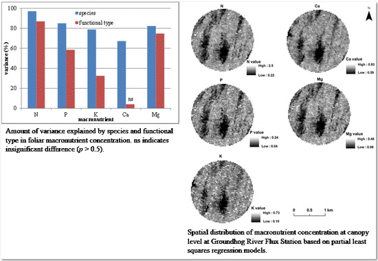
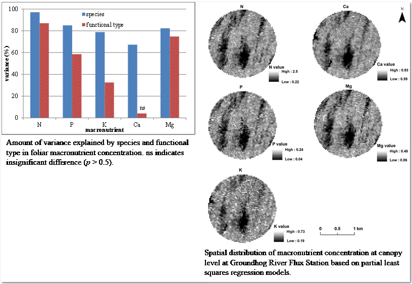
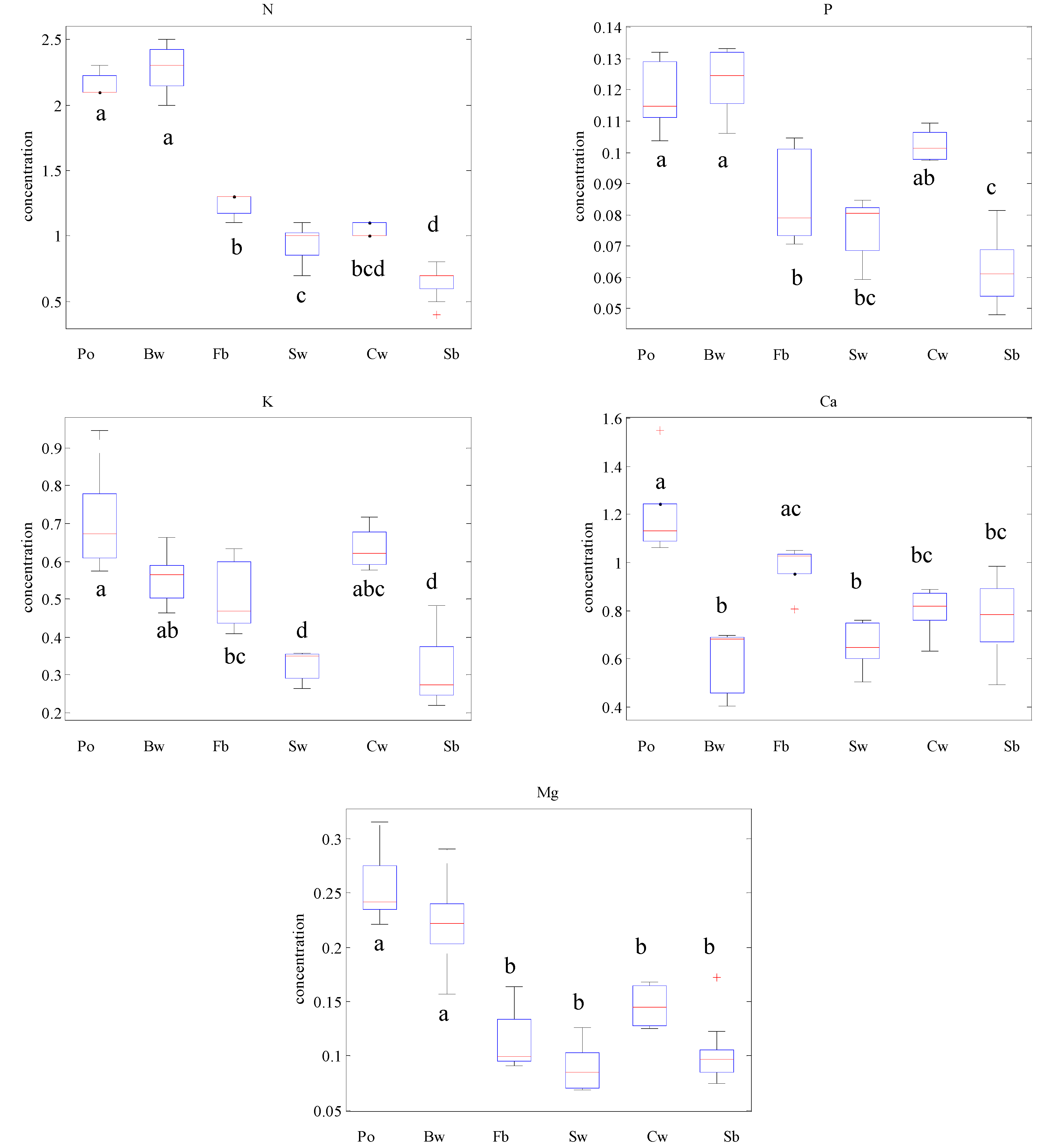
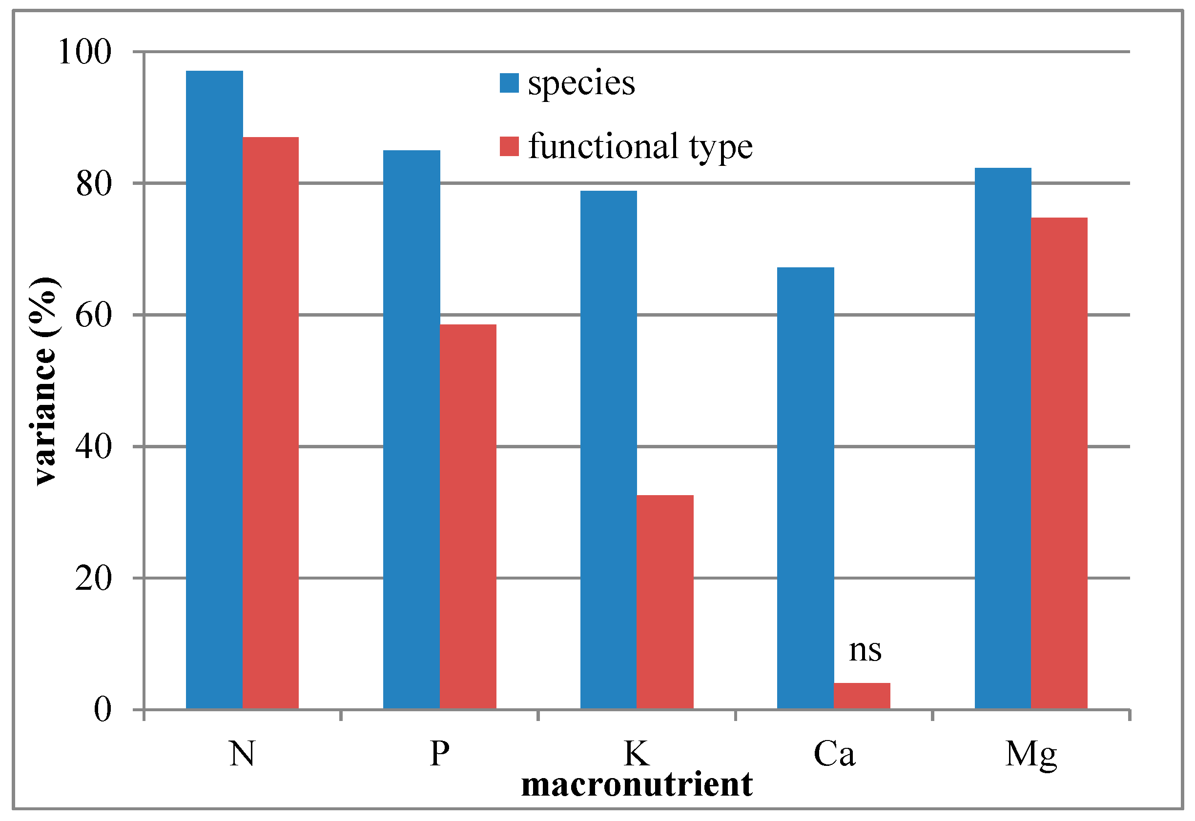
3.1. Variation of Macronutrient Concentration by Species and Functional Type

Foliar concentrations of N, P and Mg are higher for the deciduous species. Trembling aspen and white birch have significantly greater concentrations of these macronutrients than coniferous species. Black and white spruces have the lowest concentrations of these macronutrients. There is more overlap between the functional types for K and Ca foliar concentration and the difference in Ca concentration between functional types is insignificant (Figure 2).

Figure 2. Boxplots of foliar macronutrient concentration: Units of concentration are %. n = 5 for all species except black spruce (n = 13). Lowercase letters denote significant differences in macronutrient concentration among species (p ≤ 0.05). Po = trembling aspen; Bw = white birch; Fb = balsam fir; Sw = white spruce; Cw = white cedar; and Sb = black spruce.

Figure 2. Boxplots of foliar macronutrient concentration: Units of concentration are %. n = 5 for all species except black spruce (n = 13). Lowercase letters denote significant differences in macronutrient concentration among species (p ≤ 0.05). Po = trembling aspen; Bw = white birch; Fb = balsam fir; Sw = white spruce; Cw = white cedar; and Sb = black spruce.

The PCA results showed that 87% of the variance in macronutrient concentration could be explained by two principal components (Figure 3). The first component is an average of all macronutrients except Ca, which only has small contribution to the first component. The second component is dominated by Ca. It can be seen that coniferous species are clustered together at the lower end of principal component 1 indicating lower concentrations of N, P, K and Mg. Deciduous species are grouped together at the higher end of component 1 indicating that they have greater concentrations of these four macronutrients. However, deciduous species are distinctly separated from each other along component 2. This indicates that Ca concentration of trembling aspen is greater than white birch. Indeed, white birch has the lowest Ca concentration among all species. Coniferous species tend to have a gradient of Ca concentration.

Figure 3. Principal component analysis (PCA) of foliar macronutrient concentrations across species. Po = trembling aspen; Bw = white birch; Fb = balsam fir; Sw = white spruce; Cw = white cedar; and Sb = black spruce.

Figure 3. Principal component analysis (PCA) of foliar macronutrient concentrations across species. Po = trembling aspen; Bw = white birch; Fb = balsam fir; Sw = white spruce; Cw = white cedar; and Sb = black spruce.

Figure 4. Amount of variance explained by species and functional type in foliar macronutrient concentration. ns indicates insignificant difference (p > 0.5).

Figure 4. Amount of variance explained by species and functional type in foliar macronutrient concentration. ns indicates insignificant difference (p > 0.5).

Species and functional types explain most of the variance in macronutrient concentration at the foliar level. Variance ranging from 67% to 97% was explained by species; the lowest for Ca and the highest for N. Functional type explained lower macronutrient variance than species. In particular, only 4% and 33% of the variance were explained by functional type for Ca (p = 0.23) and K concentration (Figure 4).

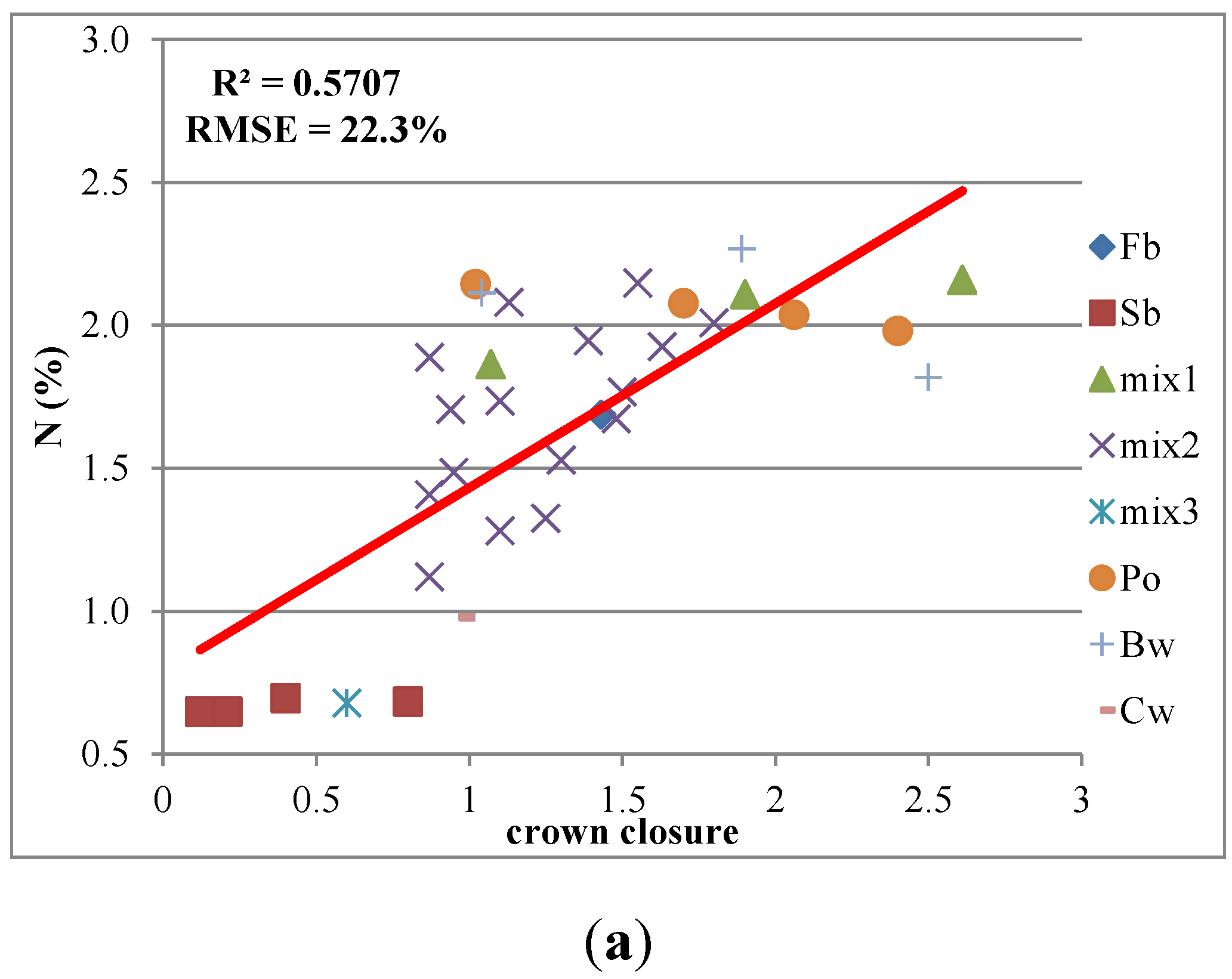
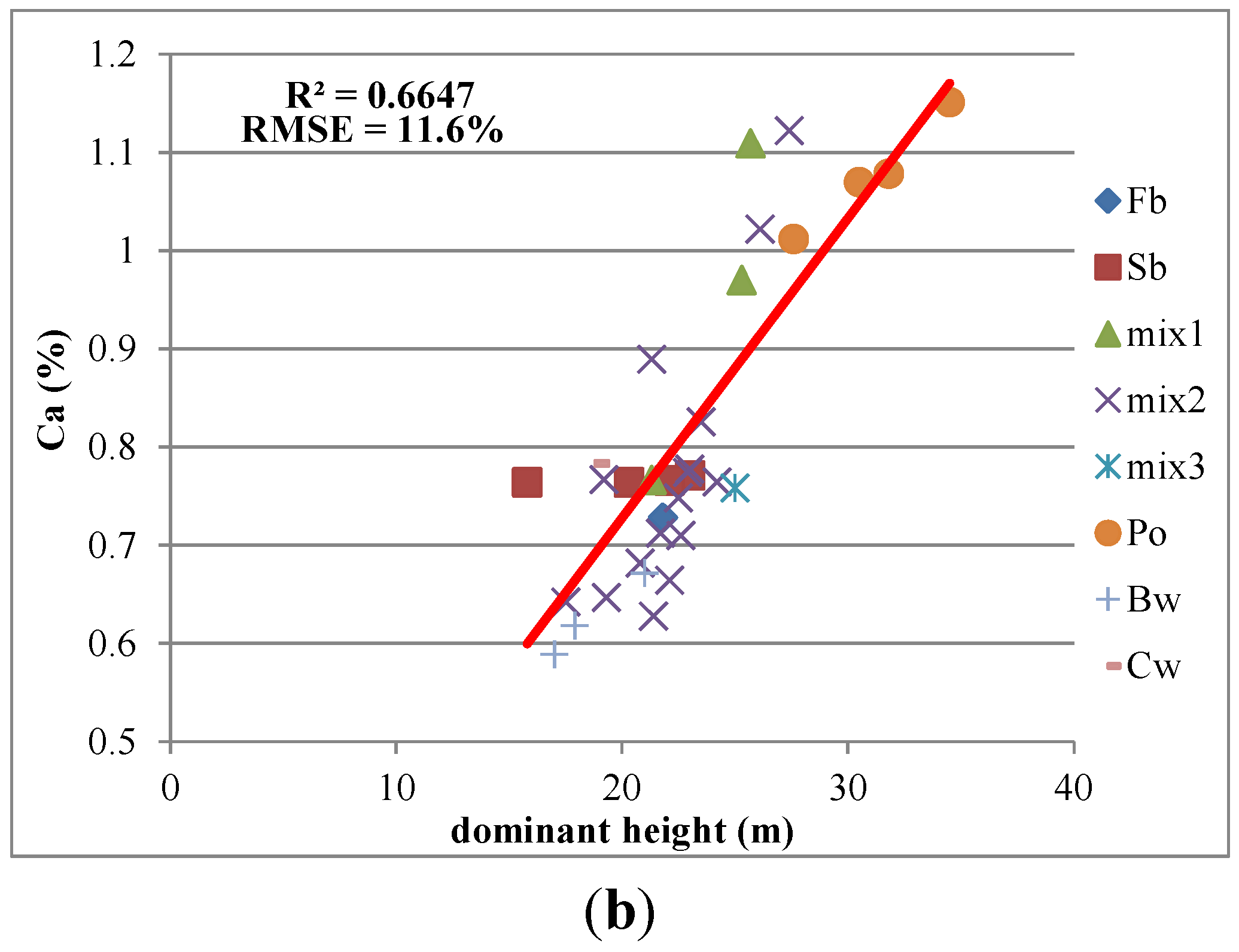
3.2. Relationships between Canopy Structure and Macronutrients

All of the macronutrients, with the exception of Ca, have significant correlation with crown closure, whereas Ca exhibits significant correlation with height, as do K and Mg (Table 1).

Table 1. Spearman’s correlation coefficients between macronutrient concentration and canopy structural metrics. Units of concentration are %. (* and ** denote significance at p < 0.01 and p < 0.0001, respectively).

	N	P	K	Ca	Mg
Dominant Height (m)	0.34	0.33	0.48**	0.71*	0.47**
Mean Dominant Height (m)	0.34	0.33	0.49**	0.70*	0.46**
Lorey's Height (m)	0.42	0.41	0.52**	0.65*	0.51**
Average Height (m)	0.32	0.30	0.41	0.48**	0.39
Crown Closure	0.74*	0.74*	0.69*	0.18	0.76*
Basal Area (m2·ha−1)	0.45**	0.46**	0.63*	0.56**	0.55**
Biomass (kg·ha−1)	0.38	0.38	0.52**	0.48**	0.48**

Table 1. Spearman’s correlation coefficients between macronutrient concentration and canopy structural metrics. Units of concentration are %. (* and ** denote significance at p < 0.01 and p < 0.0001, respectively).

	N	P	K	Ca	Mg
Dominant Height (m)	0.34	0.33	0.48**	0.71*	0.47**
Mean Dominant Height (m)	0.34	0.33	0.49**	0.70*	0.46**
Lorey's Height (m)	0.42	0.41	0.52**	0.65*	0.51**
Average Height (m)	0.32	0.30	0.41	0.48**	0.39
Crown Closure	0.74*	0.74*	0.69*	0.18	0.76*
Basal Area (m2·ha−1)	0.45**	0.46**	0.63*	0.56**	0.55**
Biomass (kg·ha−1)	0.38	0.38	0.52**	0.48**	0.48**

The relationship of macronutrients with basal area is stronger for K, Ca and Mg compared to N and P and there is no significant correlation between biomass and N and P (Table 1). When N and Ca concentration are plotted against crown closure and dominant height, the relationship of species composition and functional type with macronutrient concentration becomes clear (Figure 5). Low N levels are characteristic of plots dominated by black spruce and other coniferous species, whereas high N levels are characteristic of plots dominated by white birch, trembling aspen and their mixtures. On the other hand, white birch dominated plots represent the lowest end of the range for Ca concentration. The relationships of P, K and Mg with crown closure were very similar to that of N and crown closure.

Figure 5. The relationship between (a) N concentration and crown closure, and (b) Ca concentration and dominant height at the plot level. Red line is the linear fit. Bf = balsam fir; Sb = black spruce; Po = trembling aspen; Bw = white birch; Cw = white cedar; mix1 = mixed deciduous; mix2 = mixed deciduous and conifer; and mix3 = mixed conifer.

Figure 5. The relationship between (a) N concentration and crown closure, and (b) Ca concentration and dominant height at the plot level. Red line is the linear fit. Bf = balsam fir; Sb = black spruce; Po = trembling aspen; Bw = white birch; Cw = white cedar; mix1 = mixed deciduous; mix2 = mixed deciduous and conifer; and mix3 = mixed conifer.

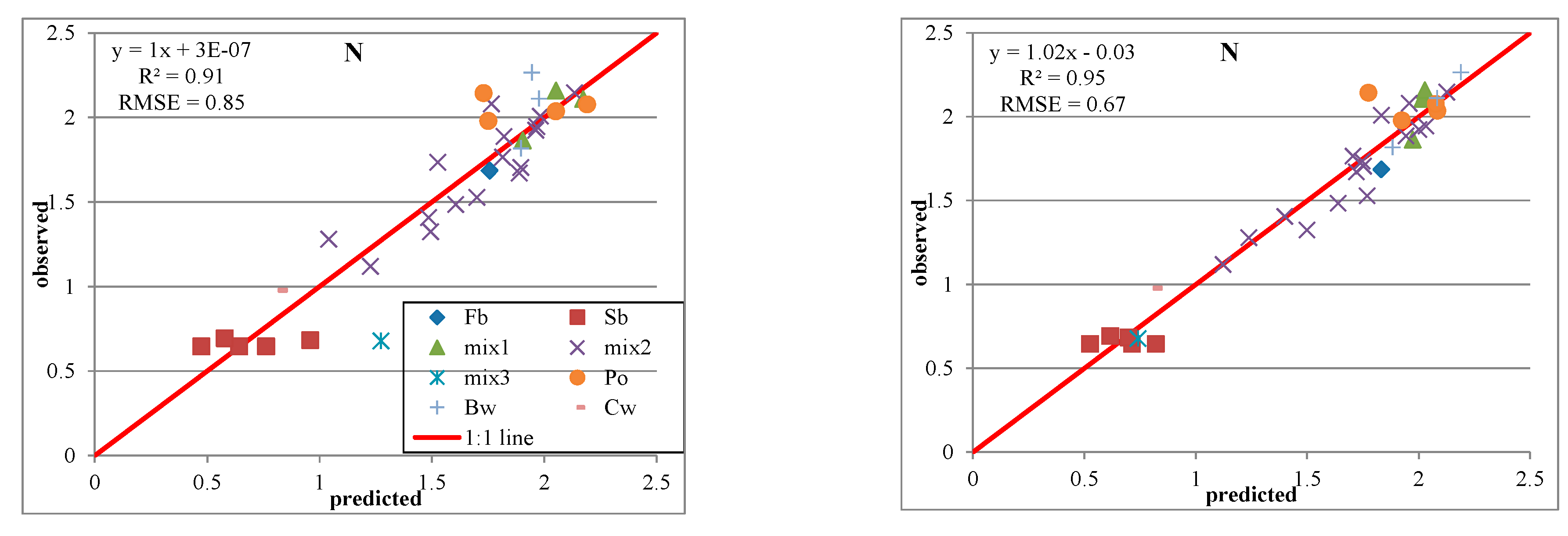
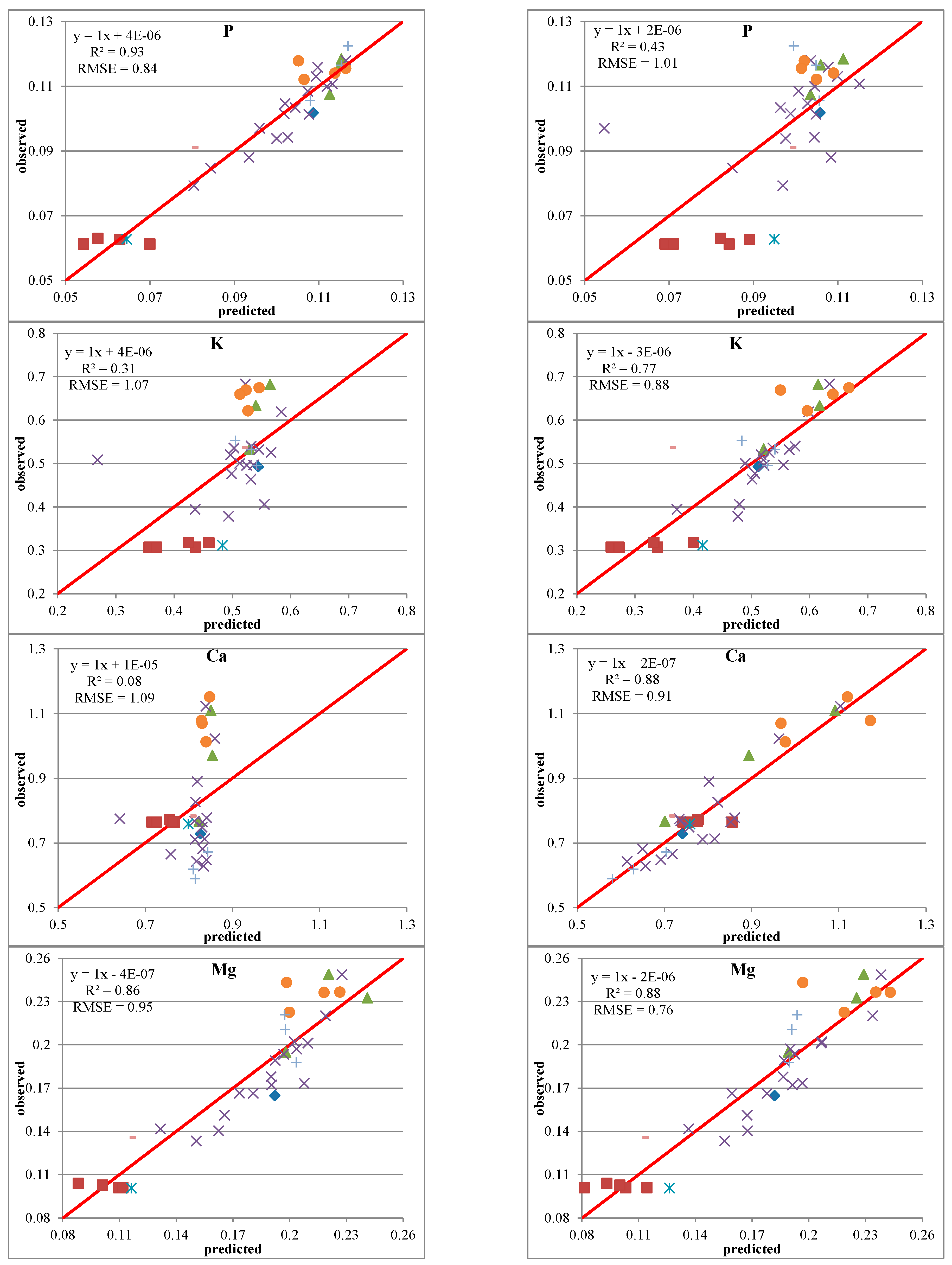
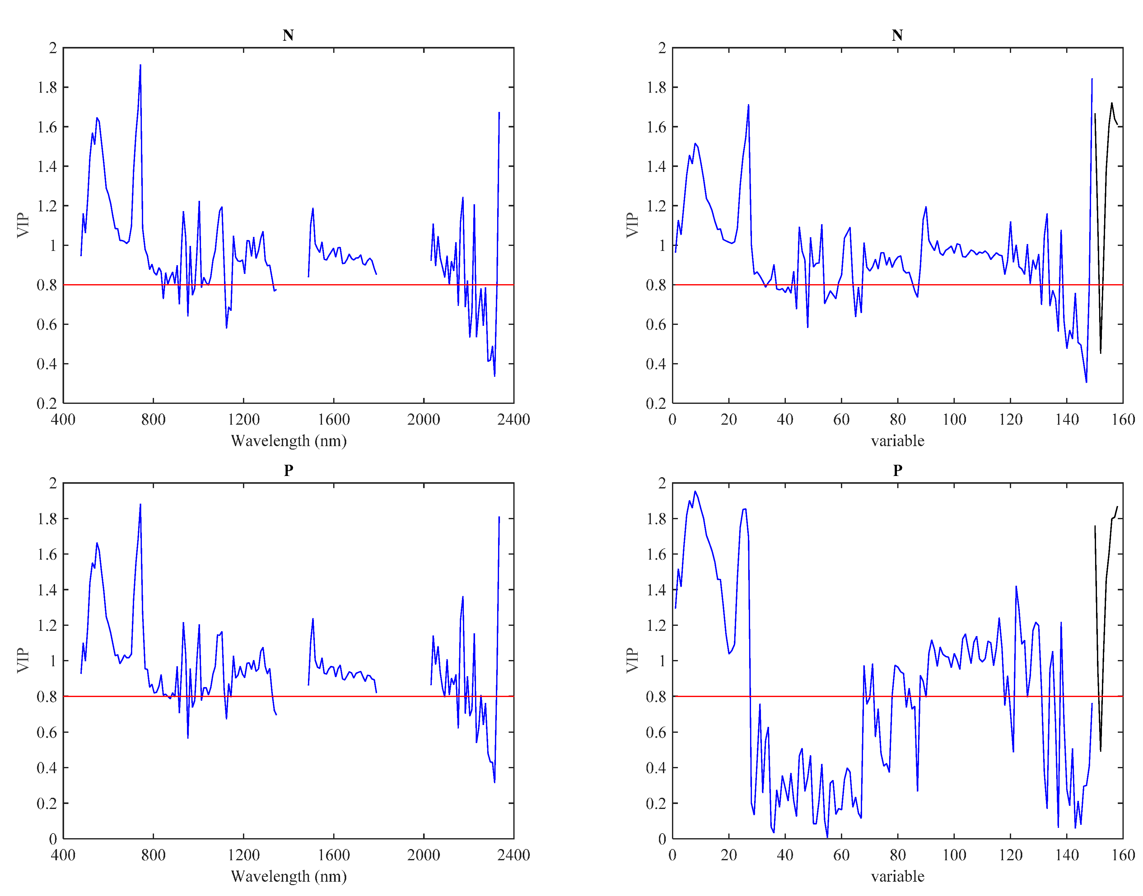
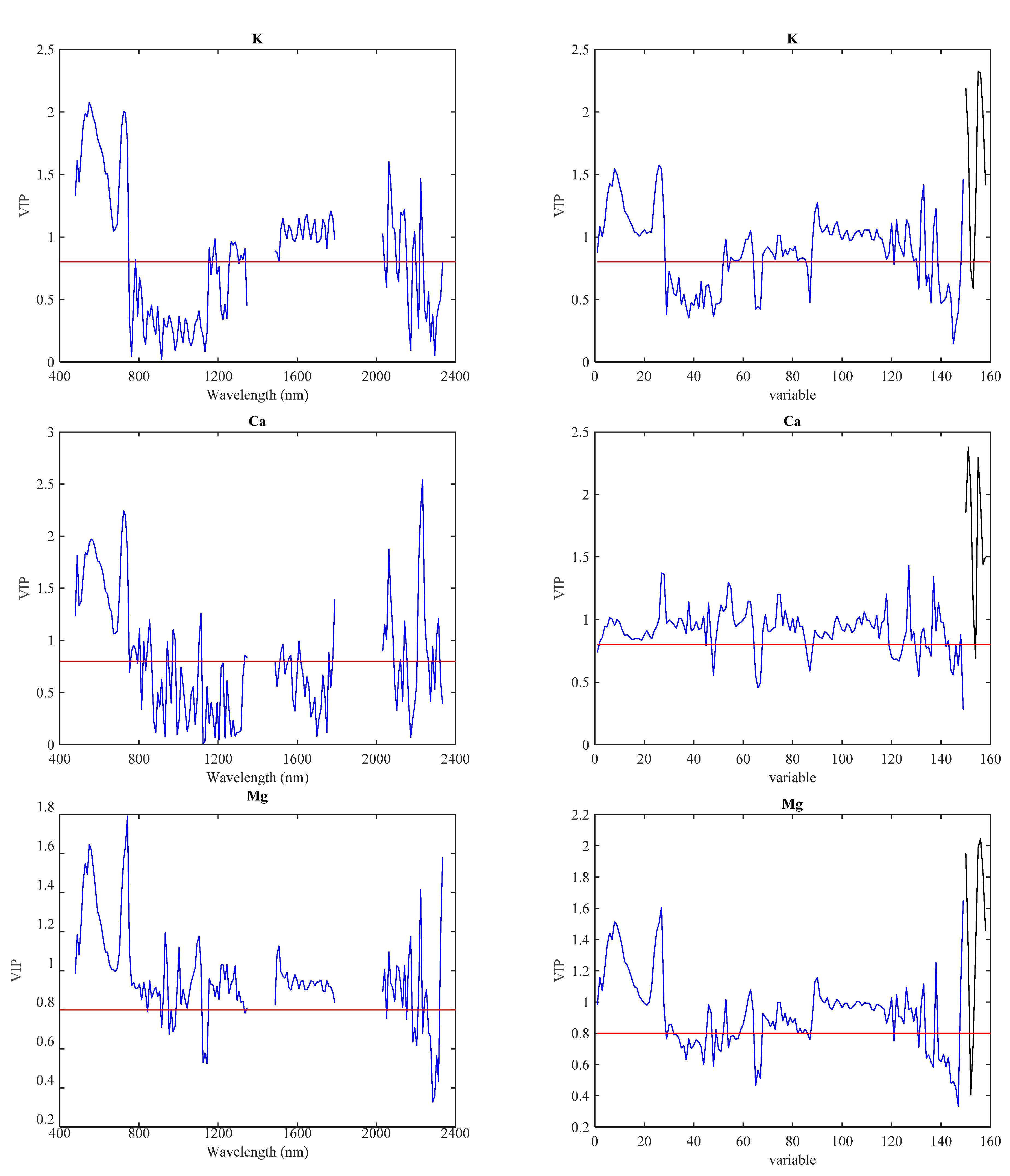
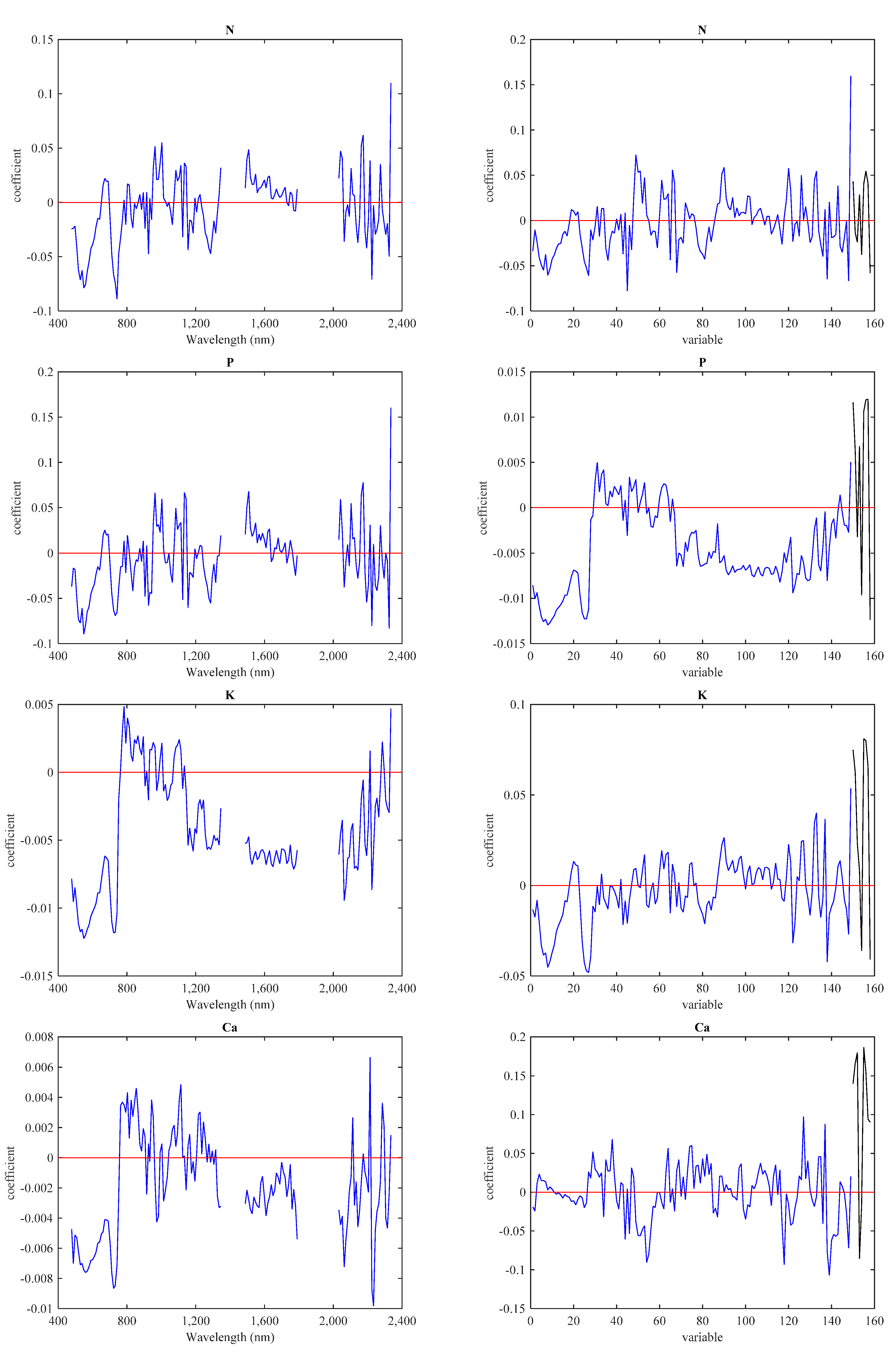
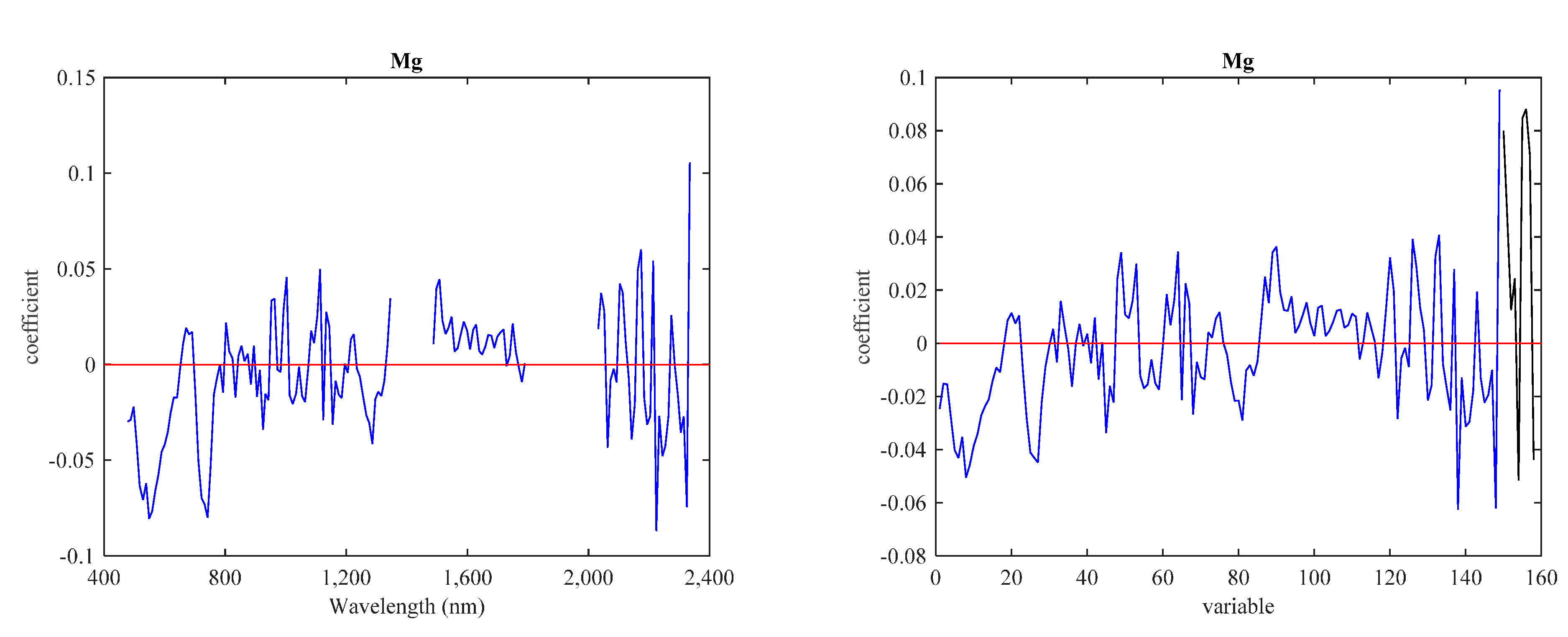
3.3. Predictive Models with IS Data

PLS models derived using Hyperion data explained 91%, 93% and 86% of the variation in canopy N, P and Mg concentrations with four, five and four factors, respectively. On the other hand, only 8% and 31% of the variation in canopy Ca and K concentrations were accounted for IS data with large prediction RMSEs (Figure 6). These graphs reflect the transition between functional types and species composition at GRFS. Basically, PLS analysis is capturing this functional type variation. Plots dominated by trembling aspen and mixtures of aspen and birch tend to cluster at the high end while plots dominated by black spruce and mixtures of the coniferous species tend to cluster at the low end of the range for N, P, K and Mg for the PLS models (Figure 6). Examination of the coefficients and VIP plots reveal that all portions of the spectrum, although with greater contributions by the visible and SWIR regions, contributed to explain the variance in concentrations of N, P and Mg (Figure 7 and Figure 8). Only visible and SWIR regions of the spectrum contributed for predicting K and Ca concentrations and the coefficients for their predictive models were two orders of magnitude smaller than the coefficients of other macronutrients’ models (Figure 7 and Figure 8).

Figure 6. Scatterplots of observed vs. predicted macronutrient concentrations. Left column shows partial least squares (PLS) model fits using only IS data and right column shows PLS model fits using IS and LiDAR data together of N, P, K, Ca and Mg, respectively. Concentration units are %. RMSEs are leave-one-out cross validation errors of standardized data. Red line indicates the 1:1 relationship. Fb = balsam fir; Sb = black spruce; Po = trembling aspen; Bw = white birch; Cw = white cedar; mix1 = mixed deciduous; mix2 = mixed deciduous and conifer; and mix3 = mixed conifer.

Figure 6. Scatterplots of observed vs. predicted macronutrient concentrations. Left column shows partial least squares (PLS) model fits using only IS data and right column shows PLS model fits using IS and LiDAR data together of N, P, K, Ca and Mg, respectively. Concentration units are %. RMSEs are leave-one-out cross validation errors of standardized data. Red line indicates the 1:1 relationship. Fb = balsam fir; Sb = black spruce; Po = trembling aspen; Bw = white birch; Cw = white cedar; mix1 = mixed deciduous; mix2 = mixed deciduous and conifer; and mix3 = mixed conifer.

Figure 7. Standardized coefficients for the partial least squares (PLS) regression predictive models. Left column shows the coefficients for the models derived using only IS data and right column shows the coefficients for the models using IS and LiDAR data together for N, P, K, Ca and Mg, respectively. The black line in the right column graphs represents LiDAR data. The x-axis in the right column graphs represents the same 149 wavelengths in the left column graphs and additionally the LiDAR data. The red line indicates zero.

Figure 7. Standardized coefficients for the partial least squares (PLS) regression predictive models. Left column shows the coefficients for the models derived using only IS data and right column shows the coefficients for the models using IS and LiDAR data together for N, P, K, Ca and Mg, respectively. The black line in the right column graphs represents LiDAR data. The x-axis in the right column graphs represents the same 149 wavelengths in the left column graphs and additionally the LiDAR data. The red line indicates zero.

Figure 8. Variable importance of projection (VIP) values for the partial least squares (PLS) regression predictive models. Left column shows the values derived using only IS data and right column shows the values using IS and LiDAR data together for N, P, K, Ca and Mg, respectively. The black line in the right column graphs represents LiDAR data. The x-axis in the right column graphs represents the same 149 wavelengths in the left column graphs and additionally the LiDAR data. The red line indicates Wold’s criterion value of 0.8.

Figure 8. Variable importance of projection (VIP) values for the partial least squares (PLS) regression predictive models. Left column shows the values derived using only IS data and right column shows the values using IS and LiDAR data together for N, P, K, Ca and Mg, respectively. The black line in the right column graphs represents LiDAR data. The x-axis in the right column graphs represents the same 149 wavelengths in the left column graphs and additionally the LiDAR data. The red line indicates Wold’s criterion value of 0.8.

3.4. Predictive Models with LiDAR Data

LiDAR models did not result in any improvement in terms of variance explained compared to the PLS models derived using IS data for N, P and Mg. However, there was significant improvement for the prediction of K and Ca using LiDAR data. The variance explained in Ca concentration by the LiDAR model was 10-fold greater than the PLS model and the prediction RMSE was the lowest among all of the macronutrients (Table 2). The reason Ca concentration is much better predicted with the LiDAR data is because dominant height follows a similar distribution across species to the foliar concentration of Ca. For instance, unlike the other macronutrients, white birch is at the lowest end of the Ca range instead of black spruce (Figure 5b). The amount of variance explained for K concentration more than doubled compared to the IS model (from 31% to 68%) with a single variable LiDAR model. Fiftieth percentile of height was consistently selected for all macronutrient predictive models and maximum height was selected in three of the models (Table 2).

Table 2. Predictive models generated from LiDAR structural metrics using multiple linear regression. RMSEs are reported as percent of the mean.

Nutrient	LiDAR Metric	R2	Adjusted R2	Residuals Shapiro		Prediction RMSE
N	50th perc. ht., max. ht.	0.71	0.69	0.97	0.37	19.5
P	50th perc. ht., max. ht.	0.65	0.63	0.96	0.30	12.9
K	50th perc. ht.	0.68	0.67	0.97	0.45	13.9
Ca	50th perc. ht., cv.	0.80	0.79	0.98	0.75	9.4
Mg	50th perc. ht., max. ht.	0.77	0.76	0.96	0.32	13.8

Table 2. Predictive models generated from LiDAR structural metrics using multiple linear regression. RMSEs are reported as percent of the mean.

Nutrient	LiDAR Metric	R2	Adjusted R2	Residuals Shapiro		Prediction RMSE
N	50th perc. ht., max. ht.	0.71	0.69	0.97	0.37	19.5
P	50th perc. ht., max. ht.	0.65	0.63	0.96	0.30	12.9
K	50th perc. ht.	0.68	0.67	0.97	0.45	13.9
Ca	50th perc. ht., cv.	0.80	0.79	0.98	0.75	9.4
Mg	50th perc. ht., max. ht.	0.77	0.76	0.96	0.32	13.8

3.5. Predictive Models with IS and LiDAR Data

Combination of IS and LiDAR in the PLS regression analysis further improved the prediction accuracy for N, K, Ca and Mg compared to models derived from only using IS and only using LiDAR data. For these macronutrients, the amount of variance explained increased and the prediction RMSEs decreased (Figure 6). However, prediction accuracy for P decreased when IS and LiDAR data were combined in the PLS regression analysis compared to models derived from only using IS and only using LiDAR data. Amount of variance decreased from 95% to 43% with increase in prediction RMSE to 1.01 from 0.84 compared to the IS models (Figure 6). Most of the LiDAR metrics contribute to explain variance in macronutrient concentrations though it is most evident in Ca and K predictions where model coefficients increased by one- to two-fold compared to the IS only models and there are sharp increases in the VIP values (Figure 7 and Figure 8). On the other hand, model coefficients decreased by two-fold and the contribution of NIR portion decreased for P prediction (Figure 7 and Figure 8).

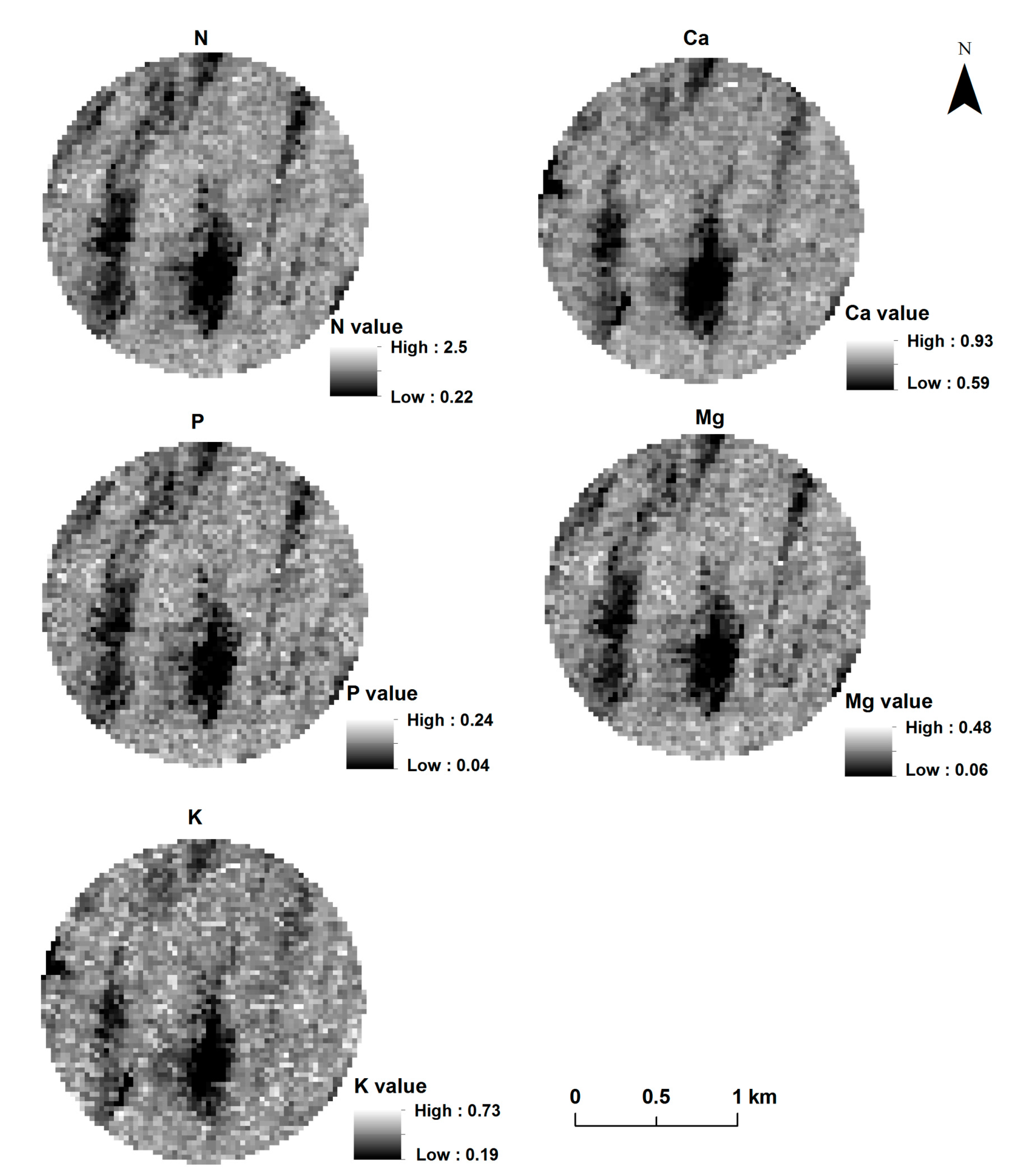
3.6. Spatial Distribution of Canopy Macronutrient Concentration

The general pattern of spatial distribution of macronutrients at the canopy of GRFS mixedwood forest is very similar (Figure 9). This pattern basically reflects the functional type distribution at the site. The areas that are low in the concentration of macronutrients are dominated by black spruce and mix of other coniferous species. Likewise, the areas that have high concentrations of macronutrients are dominated by deciduous species. The pattern appears to be slightly less evident for Ca and K for which the very low concentration areas to the north and west are diminished in size (Figure 9).

Figure 9. Spatial distribution of macronutrient concentration at canopy level at Groundhog River Flux Station (GRFS). Units of concentration are %. Maps are generated from partial least squares (PLS) regression models using Hyperion data.

Figure 9. Spatial distribution of macronutrient concentration at canopy level at Groundhog River Flux Station (GRFS). Units of concentration are %. Maps are generated from partial least squares (PLS) regression models using Hyperion data.

4. Discussion

Foliar macronutrient concentrations vary by species composition and functional types at GRFS, which agrees well with similar studies conducted in different ecosystems. McNeil et al. [48] showed that 93% of the spatial variation in foliar N was explained by species composition in temperate mixedwood forests of the Adirondack Park, New York. Similarly, 58% of the variation in foliar N was accounted for by plant community type in a Mediterranean ecosystem in California [46]. Species composition explained 66%, 60%, 63%, 57% and 60% of the variation in foliar N, P, K, Ca and Mg, respectively, in a lowland tropical forest in Borneo [50]. In Amazonian tropical forests, species composition explained 78%, 38% and 28% of the variation in foliar N, P and Ca, respectively [18]. Asner et al. [49] also determined that species were the major factor causing chemical variance in Australian tropical forests. Site characteristics including soil quality, slope, aspect, and elevation also contribute to chemical variation, which we did not account for in our study. However, from our observations we know that pure black spruce patches are found on the boggy, low-nutrient sections of the site and thus reflect the soil quality indirectly. Since the GRFS site has minimal elevation gradients, it is unlikely that site characteristics will contribute much to the variation in foliar macronutrients at the site.

Our estimates of N, P and Mg using spaceborne Hyperion data are better than the few other studies that were conducted using spectroradiometer and airborne data whereas our estimates Ca and K are worse. For example, canopy P concentration in African savannah grass was predicted with an R² of 0.63 and RMSE of 28% using airborne IS data [30]. The simple ratio vegetation index (1129 nm/462 nm) calculated from airborne IS data was correlated with P (R² = 0.65) in the forage vegetation canopy composed of grasses, sedges, forbs, sagebrush and willow in Yellowstone National Park [31]. Predictive models with R² values of 0.73, 0.67, 0.77, 0.17 and 0.33 for N, Ca, Mg, P and K, respectively, were reported for greenhouse-grown tropical grass canopies using the continuum removal technique in the 550–750 nm range using spectroradiometer data [43]. One reason for the difference between the amount of variance explained in Ca concentration between our study and this study may be related to the low correlations of Ca with other macronutrients in our dataset compared to theirs where Ca exhibited very significant correlations with N and Mg. In a previous study using spectroradiometer data and the continuum removal technique, the authors successfully modeled N, Ca, Mg, P and K concentrations (i.e., R² values of 0.70, 0.50, 0.68, 0.80 and 0.64, respectively) for a canopy of five grass species [27]. Meanwhile, Ferwerda and Skidmore [28] modeled N, Ca, Mg, P and K (R² values of 0.76, 0.65, 0.56, 0.85 and 0.73, respectively) from reflectance collected from olive, heather, willow and mopane leaf samples using stepwise regression where up to four bands were included in the models. In the studies cited so far, the prediction accuracy for Ca is consistently better than reported here. In addition to the correlation between macronutrients, this may be a result of the macronutrients having significant relationships with crown closure at GRFS. Crown closure reflects the amount of green foliage in the canopy and directly controls the spectral response collected over the canopy. Crown closure was identified as the biophysical variable linking spectral data to canopy N:P ratio over two seasons at the same site [54] and it was also found to be controlling the spectral response in jack pine stands of northern Ontario, Canada [69].

Observed vs. predicted graphs of PLS models reflect the transition between functional types and species composition at GRFS. Basically, PLS analysis is capturing this functional type variation. The relationship between LiDAR and macronutrients is also based on the canopy biophysical variables, which display a gradient across functional types. The reason Ca concentration is much better predicted with the LiDAR data is because dominant height follows a similar distribution across species to the foliar concentration of Ca. This is clearly visible in the observed Ca vs. dominant height graph across plots. For instance, unlike the other macronutrients, white birch is at the lowest end of the Ca range instead of black spruce (Figure 5b).

Spatial distribution of canopy macronutrient concentration at GRFS mimics the functional type variation and thus, the spatial patterns of macronutrients are driven by the functional types’ distribution at the site. Forest type variation was also found to be the underlying factor in explaining the observed spatial patterns of canopy N:P ratio at this site [54].

The combination of IS and LiDAR data improved the prediction accuracy of N, K, Ca and Mg with very significant improvements especially for Ca and K. This is very important because information on the spatial distribution of these macronutrients at the canopy scale will allow researchers and forest managers to assess forest condition and stress and use this information to relate it to ecosystem processes such as forest nutrient cycling and C exchange.

The ability to predict N, P and Mg concentration at the canopy scale using spaceborne IS data is very encouraging as it demonstrates the potential for mapping these macronutrients at the canopy scale across large geographic areas at lower cost. This study is a precursor to the feasibility of canopy scale macronutrient mapping across large regions of forest harvesting in the mixedwood boreal forest, which is not too far given the planned satellite IS missions to be launched within this decade such as NASA’s HyspIRI and ESA’s EnMAP. The data from these sensors will have higher SNR, and temporal and spatial resolution than currently available making it more likely to have success at predicting macronutrients.

We used airborne LiDAR and spaceborne IS data (i.e., Hyperion) in this study. Both have limited geographic coverage since availability is based on user request. LiDAR data are costly to acquire. Hyperion data have low SNR, require significant preprocessing. These factors limit their widespread use by researchers. Given the cost disadvantage and geographic limitation of airborne LiDAR data, spaceborne LiDAR data such as Geoscience Laser Altimeter System (GLAS) should be tested to predict macronutrients. This study was conducted at one site representing the mixedwood boreal forest. It remains to be seen whether some canopy structural metrics can be identified linking foliar chemistry and remote sensing data in other ecosystems as well. Despite being collected two years prior to foliage sampling, the LiDAR data to macronutrients relationship is still strong because the canopy structure and height do not change substantially over that time period.

One unexpected result of the study was the decrease in the prediction accuracy of P when IS and LiDAR data were combined. This is perplexing given the fact that P can actually be predicted with moderate accuracy (R² = 0.63, prediction RMSE = 13%) using LiDAR data and with very high accuracy with IS data alone (R² = 0.93, standardized prediction RMSE = 0.84). This needs to be tested in other studies to see whether similar results are obtained.

Currently, scientific community is limited by the quality and continuous availability of IS data. There will be big strides in the field of canopy chemistry research if high quality and continuous IS data become available along with improvements in the methods to analyze spaceborne LiDAR data.

5. Conclusions

This study has examined the utility of spaceborne IS and airborne LiDAR data for modeling canopy macronutrient (N, P, K, Mg and Ca) concentrations in a mixedwood boreal forest. The mechanism that underlies the relationship between IS and LiDAR data and macronutrient concentration is the variation in macronutrient concentrations generated by interspecific and functional type differences at the site. Specifically, crown closure and canopy height are the structural metrics that determine the relationship between macronutrient concentration and IS and LiDAR data, respectively. Spaceborne IS (i.e., Hyperion) data accounted for 91%, 93% and 86% of the variation in canopy N, P and Mg concentration, respectively. Combination of IS and airborne LiDAR data significantly improved the prediction accuracy of canopy Ca and K concentration but decreased the prediction accuracy of canopy P concentration. Using only LiDAR data, variance ranging from 65% to 80% in macronutrient concentration could be explained. The spatial distribution of macronutrient concentration at the canopy scale mimics functional type distribution at the site. The ability to predict canopy macronutrients using only IS, only LiDAR or their combination demonstrates the potential for mapping these macronutrients at the canopy scale across larger geographic areas with the availability of high quality, spatially and temporally continuous IS data such as HyspIRI and EnMAP planned to be launched within this decade and by using spaceborne LiDAR data such as GLAS. Studies testing spaceborne IS and LiDAR data should be conducted to predict macronutrients and other biochemicals in other ecosystems.

References

1. Taiz, L.; Zeiger, E. Plant Physiology, 5th ed.; Sinauer Associates Inc.: Sunderland, MA, USA, 2010. [Google Scholar]
2. Melillo, J.M.; Aber, J.D.; Muratore, J.M. Nitrogen and lignin control of hardwood leaf litter decomposition dynamics. Ecology 1982, 63, 621–626. [Google Scholar] [CrossRef]
3. Smith, M.L.; Ollinger, S.V.; Martin, M.E.; Aber, J.D.; Hallett, R.A.; Goodale, C.L. Direct estimation of aboveground forest productivity through hyperspectral remote sensing of canopy nitrogen. Ecol. Appl. 2002, 12, 1286–1302. [Google Scholar] [CrossRef]
4. Chapin, F.S. The mineral nutrition of wild plants. Annu. Rev. Ecol. Syst. 1980, 11, 233–260. [Google Scholar] [CrossRef]
5. Marschner, H. Mineral Nutrition of Higher Plants, 2nd ed.; Academic Press: San Diego, CA, USA, 1995. [Google Scholar]
6. Mengel, K.; Kirkby, E.A. Principles of Plant Nutrition, 5th ed.; Kluwer Academic Publishers: Dordrecht, The Netherlands, 2001. [Google Scholar]
7. Hepler, P.K. Calcium: A central regulator of plant growth and development. Plant Cell 2005, 17, 2142–2155. [Google Scholar] [CrossRef] [PubMed]
8. Olivier, J.G.J.; Janssens-Maenhout, G.; Peters, J.A.H.W.; Wilson, J. Long-Term Trend in Global CO2 Emissions 2011 Report; PBL/JRC: The Hague, The Netherlands, 2011. [Google Scholar]
9. Ollinger, S.V.; Smith, M.L. Net primary production and canopy nitrogen in a temperate forest landscape: An analysis using imaging spectroscopy, modeling, and field data. Ecosystems 2005, 8, 1–19. [Google Scholar] [CrossRef]
10. Coops, N.C.; Smith, M.L.; Martin, M.E.; Ollinger, S.V. Prediction of eucalypt foliage nitrogen content from satellite-derived hyperspectral data. IEEE Trans. Geosci. Remote Sens. 2003, 41, 1338–1346. [Google Scholar] [CrossRef]
11. Smith, M.L.; Martin, M.E.; Ollinger, S.V.; Plourde, L. Analysis of hyperspectral data for estimation of temperate forest canopy nitrogen concentration: Comparison between an airborne (AVIRIS) and a spaceborne (Hyperion) sensor. IEEE Trans. Geosci. Remote Sens. 2003, 41, 1332–1337. [Google Scholar] [CrossRef]
12. Townsend, P.A.; Foster, J.R.; Chastain, R.A., Jr.; Currie, W.S. Application of imaging spectroscopy to mapping canopy nitrogen in the forests of the central Appalachian Mountains using Hyperion and AVIRIS. IEEE Trans. Geosci. Remote Sens. 2003, 41, 1347–1354. [Google Scholar] [CrossRef]
13. Wessman, C.A.; Aber, J.D.; Peterson, D.L.; Melillo, J.M. Remote sensing of canopy chemistry and nitrogen cycling in temperate forest ecosystems. Nature 1988, 335, 154–156. [Google Scholar] [CrossRef]
14. Curran, P.J.; Kupiec, J.A.; Smith, G.M. Remote sensing the biochemical composition of a slash pine canopy. IEEE Trans. Geosci. Remote Sens. 1997, 35, 415–420. [Google Scholar] [CrossRef]
15. Martin, M.E.; Aber, J.D. High spectral resolution remote sensing of forest canopy lignin, nitrogen, and ecosystem processes. Ecol. Appl. 1997, 7, 431–444. [Google Scholar] [CrossRef]
16. Wicklein, H.F.; Ollinger, S.V.; Martin, M.E.; Hollinger, D.Y.; Lepine, L.C.; Day, M.E.; Bartlett, M.K.; Richardson, A.D.; Norby, R.J. Variation in foliar nitrogen and albedo in response to nitrogen fertilization and elevated CO2. Oecologia 2012, 169, 915–925. [Google Scholar] [CrossRef] [PubMed]
17. Carlson, K.M.; Asner, G.P.; Hughes, R.F.; Ostertag, R.; Martin, R.E. Hyperspectral remote sensing of canopy biodiversity in Hawaiian lowland rainforests. Ecosystems 2007, 10, 536–549. [Google Scholar] [CrossRef]
18. Asner, G.P.; Martin, R.E.; Tupayachi, R.; Anderson, C.B.; Sinca, F.; Carranza-Jimenez, L.; Martinez, P. Amazonian functional diversity from forest canopy chemical assembly. Proc. Natl. Acad. Sci. USA 2014, 111, 5604–5609. [Google Scholar] [CrossRef] [PubMed]
19. Asner, G.P. Hyperspectral remote sensing of canopy chemistry, physiology, and biodiversity in tropical rainforests. In Hyperspectral Remote Sensing of Tropical and Sub-Tropical Forests; Kalacska, M., Sanches-Azofeifa, G.A., Eds.; CRC Press: Boca Raton, FL, USA, 2008; pp. 261–296. [Google Scholar]
20. Kokaly, R.F.; Asner, G.P.; Ollinger, S.V.; Martin, M.E.; Wessman, C.A. Characterizing canopy biochemistry from imaging spectroscopy and its application to ecosystem studies. Remote Sens. Environ. 2009, 113, S78–S91. [Google Scholar] [CrossRef]
21. Ollinger, S.V.; Richardson, A.D.; Martin, M.E.; Hollinger, D.Y.; Frolking, S.E.; Reich, P.B.; Katul, G.G.; Mungere, J.W.; Orend, R.; Smith, M.-L.; et al. Canopy nitrogen, carbon assimilation, and albedo in temperate and boreal forests: Functional relations and potential climate feedbacks. Proc. Natl. Acad. Sci. USA 2008, 105, 19336–19341. [Google Scholar] [CrossRef] [PubMed]
22. Knyazikhin, Y.; Schull, M.A.; Stenberg, P.; Mottus, M.; Rautiainen, M.; Yang, Y.; Marshak, A.; Carmona, P.L.; Kaufmanna, R.K.; Lewis, P.; et al. Hyperspectral remote sensing of foliar nitrogen content. Proc. Natl. Acad. Sci. USA 2012, 110, E185–E192. [Google Scholar] [CrossRef] [PubMed]
23. Al-Abbas, A.H.; Barr, R.; Hall, J.D.; Crane, F.L.; Baumgardner, M.F. Spectra of normal and nutrient deficient maize leaves. Agron. J. 1974, 66, 16–20. [Google Scholar] [CrossRef]
24. Osborne, S.L.; Schepers, J.S.; Francis, D.D.; Schlemmer, M.R. Detection of phosphorous and nitrogen deficiencies in corn using spectral radiance measurements. Agron. J. 2002, 94, 1215–1221. [Google Scholar] [CrossRef]
25. Gong, P.; Pu, R.; Heald, R.C. Analysis of in situ hyperspectral data for nutrient estimation of giant sequoia. Int. J. Remote Sens. 2002, 23, 1827–1850. [Google Scholar] [CrossRef]
26. Ponzoni, F.J.; de M. Gonçalves, J.L. Spectral features associated with nitrogen, phosphorus, and potassium deficiencies in Eucalyptus saligna seedling leaves. Int. J. Remote Sens. 1999, 20, 2249–2264. [Google Scholar] [CrossRef]
27. Mutanga, O.; Skidmore, A.K.; Prins, H.H.T. Predicting in situ pasture quality in the Kruger National Park, South Africa, using continuum-removed absorption features. Remote Sens. Environ. 2004, 89, 393–408. [Google Scholar] [CrossRef]
28. Ferwerda, J.G.; Skidmore, A.K. Can nutrient status of four woody plant species be predicted using field spectrometry? ISPRS J. Photogramm. Remote Sens. 2007, 62, 406–414. [Google Scholar] [CrossRef]
29. Porder, S.; Asner, G.P.; Vitousek, P.M. Ground-based and remotely sensed nutrient availability across a tropical landscape. Proc. Natl. Acad. Sci. USA 2005, 102, 10909–10912. [Google Scholar] [CrossRef] [PubMed]
30. Mutanga, O.; Kumar, L. Estimating and mapping grass phosphorus concentration in an African savanna using hyperspectral image data. Int. J. Remote Sens. 2007, 28, 4897–4911. [Google Scholar] [CrossRef]
31. Mirik, M.; Norland, J.E.; Crabtree, R.L.; Biondini, M.E. Hyperspectral one-meter-resolution remote Sensing in Yellowstone National Park, Wyoming: I. Forage nutritional values. Rangel. Ecol. Manag. 2005, 58, 452–458. [Google Scholar] [CrossRef]
32. NASA HyspIRI Mission Website. Available online: http://hyspiri.jpl.nasa.gov (accessed on 9 April 2015).
33. EnMAP Website. Available online: http://www.enmap.org/sites/default/files/pdf/pub/EnMAP_komplett_web_eng.pdf (accessed on 14 April 2015).
34. Curran, P.J. Remote sensing of foliar chemistry. Remote Sens. Environ. 1989, 30, 271–278. [Google Scholar] [CrossRef]
35. Kokaly, R.F.; Clark, R.N. Spectroscopic determination of leaf biochemistry using band-depth analysis of absorption features and stepwise multiple linear regression. Remote Sens. Environ. 1999, 67, 267–287. [Google Scholar] [CrossRef]
36. Yoder, B.J.; Pettigrew-Cosby, R.E. Predicting nitrogen and chlorophyll content and concentrations from reflectance spectra (400–2500 nm) at leaf and canopy scales. Remote Sens. Environ. 1995, 53, 199–211. [Google Scholar] [CrossRef]
37. Asner, G.P. Biophysical and biochemical sources of variability in canopy reflectance. Remote Sens. Environ. 1998, 64, 234–253. [Google Scholar] [CrossRef]
38. Ollinger, S.V. Sources of variability in canopy reflectance and the convergent properties of plants. New Phytol. 2011, 189, 375–394. [Google Scholar] [CrossRef] [PubMed]
39. Dixit, L.; Ram, S. Quantitative analysis by derivative electronic spectroscopy. Appl. Spectrosc. Rev. 1985, 21, 311–418. [Google Scholar] [CrossRef]
40. Elvidge, C.D.; Chen, Z. Comparison of broad-band and narrow-band red and near-infrared vegetation indices. Remote Sens. Environ. 1995, 54, 38–48. [Google Scholar] [CrossRef]
41. Curran, P.J.; Dungan, J.L.; Peterson, D.L. Estimating the foliar biochemical concentration of leaves with reflectance spectrometry-testing the Kokaly and Clark methodologies. Remote Sens. Environ. 2001, 76, 349–359. [Google Scholar] [CrossRef]
42. Huang, Z.; Turner, B.J.; Dury, S.J.; Wallis, I.R.; Foley, W.J. Estimating foliage nitrogen concentration from HYMAP data using continuum removal analysis. Remote Sens. Environ. 2004, 93, 8–29. [Google Scholar] [CrossRef]
43. Mutanga, O.; Skidmore, A.K.; Kumar, L.; Ferwerda, J. Estimating tropical pasture quality at canopy level using band depth analysis with continuum removal in the visible domain. Int. J. Remote Sens. 2005, 26, 1093–1108. [Google Scholar] [CrossRef]
44. Kramer, R. Chemometric Techniques for Quantitative Analysis; Marcel Dekker: New York, NY, USA, 1998. [Google Scholar]
45. Feilhauer, H.; Asner, G.P.; Marten, R.E.; Schmidtlein, S. Brightness-normalized Partial Least Squares Regression for hyperspectral data. J. Quant. Spectrosc. Radiat. Transf. 2010, 111, 1947–1957. [Google Scholar] [CrossRef]
46. Dahlin, K.M.; Asner, G.P.; Field, C.B. Environmental and community controls on plant canopy chemistry in a Mediterranean-type ecosystem. Proc. Natl. Acad. Sci. USA 2013, 110, 6895–6900. [Google Scholar] [CrossRef] [PubMed]
47. Mitchell, J.; Glenn, N.; Sankey, T.; Derryberry, D.W.; Germino, M. Remote sensing of sagebrush canopy nitrogen. Remote Sens. Environ. 2012, 124, 217–223. [Google Scholar] [CrossRef]
48. McNeil, B.E.; Read, J.M.; Sullivan, T.J.; McDonnell, T.C.; Fernandez, I.J.; Driscoll, C.T. The spatial pattern of nitrogen cycling in the Adirondack Park, New York. Ecol. Appl. 2008, 18, 438–452. [Google Scholar] [CrossRef] [PubMed]
49. Asner, G.P.; Martin, R.E.; Ford, A.J.; Metcalfe, D.J.; Liddell, M.J. Leaf chemical and spectral diversity of Australian tropical forests. Ecol. Appl. 2009, 19, 236–253. [Google Scholar] [CrossRef] [PubMed]
50. Asner, G.P.; Martin, R.E.; Suhaili, A. Sources of canopy chemical and spectral diversity in lowland Bornean forest. Ecosystems 2012, 15, 504–517. [Google Scholar] [CrossRef]
51. Wright, I.J.; Reich, P.B.; Westoby, M.; Ackerly, D.D.; Baruch, Z.; Bongers, F.; Cavender-Bares, J.; Chapin, T.; Cornelissen, J.H.C.; Diemer, M.; et al. The worldwide leaf economics spectrum. Nature 2004, 428, 821–827. [Google Scholar] [CrossRef] [PubMed]
52. Reich, P.B.; Walters, M.B.; Ellsworth, D.S. From tropics to tundra: Global convergence in plant functioning. Proc. Natl. Acad. Sci. USA 1997, 94, 13730–13734. [Google Scholar] [CrossRef] [PubMed]
53. Asner, G.P.; Martin, R.E.; Carranza-Jimenez, L.; Sinca, F.; Tupayachi, R.; Anderson, C.B.; Martinez, P. Functional and biological diversity of foliar spectra in tree canopies throughout the Andes to Amazon region. New Phytol. 2014, 204, 127–139. [Google Scholar] [CrossRef] [PubMed]
54. Gökkaya, K.; Thomas, V.; Noland, T.; McCaughey, H.; Morrison, I.; Treitz, P. Mapping continuous forest type variation by means of correlating remotely sensed metrics to canopy N:P ratio in a boreal mixedwood forest. Appl. Veg. Sci. 2015, 18, 143–157. [Google Scholar] [CrossRef]
55. Thomas, V.; Treitz, P.; McCaughey, J.H.; Noland, T.; Rich, L. Canopy chlorophyll concentration estimation using hyperspectral and LiDAR data for a boreal mixedwood forest in northern Ontario, Canada. Int. J. Remote Sens. 2008, 29, 1029–1052. [Google Scholar] [CrossRef]
56. Korhonen, L.; Korpela, I.; Heiskanen, J.; Maltamo, M. Airborne discrete-return LiDAR data in the estimation of vertical canopy cover, angular canopy closure and leaf area index. Remote Sens. Environ. 2011, 115, 1065–1080. [Google Scholar]
57. Vepakomma, U.; St-Onge, B.; Kneeshaw, D. Response of a boreal forest to canopy opening: Assessing vertical and lateral tree growth with multi-temporal LiDAR data. Ecol. Appl. 2011, 21, 99–121. [Google Scholar] [CrossRef] [PubMed]
58. Magnussen, S.; Wulder, M. Post-fire canopy height recovery in Canada’s boreal forests using Airborne Laser Scanner (ALS). Remote Sens. 2012, 4, 1600–1616. [Google Scholar] [CrossRef]
59. Bolton, D.K.; Coops, N.C.; Wulder, M.A. Measuring forest structure along productivity gradients in the Canadian boreal with small-footprint Lidar. Environ. Monit. Assess. 2013, 185, 6617–6634. [Google Scholar] [CrossRef] [PubMed]
60. Li, J.; Hu, B.; Noland, T.L. Classification of tree species based on structural features derived from high density LiDAR data. Agric. For. Meteorol. 2013, 171–172, 104–114. [Google Scholar] [CrossRef]
61. Van Leeuwen, M.; Nieuwenhuis, M. Retrieval of forest structural parameters using LiDAR remote sensing. Eur. J. For. Res. 2010, 129, 749–770. [Google Scholar] [CrossRef]
62. Gökkaya, K.; Thomas, V.; Noland, T.; McCaughey, H.; Treitz, P. Testing the robustness of predictive models for chlorophyll generated from spaceborne imaging spectroscopy data for a mixedwood boreal forest canopy. Int. J. Remote Sens. 2014, 35, 218–233. [Google Scholar] [CrossRef]
63. National Forest Inventory Ground Sampling Guidelines, version 4.0. Available online: http://www.proprights.org/PDFs/workshop_2011/References/Forest%20Humus/GroundSamplingGuidelines_v.4.0._back.pdf (accessed on 31 August 2013).
64. Alemdag, I.S. Mass Equations and Merchantability Factors for Ontario Softwoods; Information Report PI-X-23; Canadian Forest Service: Chalk River, ON, Canada, 1983.
65. Alemdag, I.S. Total Tree and Merchantable Stem Biomass Equations for Ontario Hardwoods; Information Report PI-X-46; Canadian Forestry Service: Chalk River, ON, Canada, 1984.
66. Optech Inc. ALTM 2050 Airborne Laser Terrain Mapper on-line technical specifications document. Available online: http://als.nyme.hu/fileadmin/dokumentumok/als/Leirasok/Optech_ALTM_2050.pdf (accessed on 9 April 2015).
67. Thomas, V.; Treitz, P.; McCaughey, J.H.; Noland, T.; Morrison, I. Mapping stand-level forest biophysical variables for a mixedwood boreal forest using lidar: an examination of scanning density. Can. J. For. Res. 2006, 36, 34–47. [Google Scholar] [CrossRef]
68. Wold, S. PLS for multivariate linear modeling. In Chemometric Methods in Molecular Design (Methods and Principles in Medicinal Chemistry); de Vaterbeemd, H., Ed.; Verlag-Chemie: Weinheim, Germany, 1984; pp. 195–218. [Google Scholar]
69. Croft, H.; Chen, J.M.; Noland, T.L. Stand age effects on Boreal forest physiology using a long time-series of satellite data. For. Ecol. Manag. 2014, 328, 202–208. [Google Scholar] [CrossRef]