Article

Characterising the Land Surface Phenology of Europe Using Decadal MERIS Data

by
Victor F. Rodriguez-Galiano
1,2,*,
Jadunandan Dash
2 and
Peter M. Atkinson
2,3,4,5
1
Physical Geography and Regional Geographic Analysis, University of Seville, Seville 41004, Spain
2
Global Environmental Change and Earth Observation Research Group, Geography and Environment, University of Southampton, Southampton SO17 1BJ, UK
3
Faculty of Science and Technology, Engineering Building, Lancaster University, Lancaster LA1 4YR, UK
4
Faculty of Geosciences, University of Utrecht, Heidelberglaan 2, Utrecht 3584 CS, The Netherlands
5
School of Geography, Archaeology and Palaeoecology, Queen’s University Belfast, Belfast BT7 1NN, Northern Ireland, UK
*
Author to whom correspondence should be addressed.
Remote Sens. 2015, 7(7), 9390-9409; https://doi.org/10.3390/rs70709390
Submission received: 5 April 2015 / Revised: 9 July 2015 / Accepted: 15 July 2015 / Published: 22 July 2015

Abstract

:
Land surface phenology (LSP), the study of the timing of recurring cycles of changes in the land surface using time-series of satellite sensor-derived vegetation indices, is a valuable tool for monitoring vegetation at global and continental scales. Characterisation of LSP and its spatial variation is required to reveal and predict ongoing changes in Earth system dynamics. This study presents and analyses the LSP of the pan-European continent for the last decade, considering three phenological metrics: onset of greenness (OG), end of senescence (EOS), and length of season (LS). The whole time-series of Multi-temporal Medium Resolution Imaging Spectrometer (MERIS) Terrestrial Chlorophyll Index (MTCI) data at 1 km spatial resolution was used to estimate the phenological metrics. Results show a progressive pattern in phenophases from low to high latitudes. OG dates are distributed widely from the end of December to the end of May. EOS dates range from the end of May to the end of January and the spatial distribution is generally the inverse of that of the OG. Shorter growing seasons (approximately three months) are associated with rainfed croplands in Western Europe, and forests in boreal and mountainous areas. Maximum LS values appear in the Atlantic basin associated with grasslands. The LSP maps presented in this study are supported by the findings of a previous study where OG and EOS estimates were compared to those of the pan-European phenological network at certain locations corresponding to numerous observations of deciduous tree plant species. Moreover, the spatio-temporal pattern of the OG and EOS produced close agreement with the dates of deciduous tree leaf unfolding and autumnal colouring, respectively (pseudo R-squared equal to 0.70 and 0.71 and root mean square error of six days (over 365 days)).

Graphical Abstract

1. Introduction

Phenology, the study of the timing of recurring biological cycles, has emerged as an important scientific research focus as vegetation phenological events are regarded as one of the indicators of climate change [1,2,3]. All vegetation phenological events, such as emergence of the first leaf, flowerin,g or senescence, occur at a specific time depending upon the species, and local environmental and climatic conditions of the current and preceding months. In northern latitude regions such as Europe, temperature is one of the main drivers regulating vegetation phenological events. Thus, changes in temperature as a consequence of global warming may lead to changes in the timing of phenological events [4]. In addition, vegetation phenology is of paramount importance for the understanding of ecosystem functioning, playing an important role in gas and energy fluxes, surface albedo, and species interactions [5,6,7]. Given the pivotal role of this aspect of vegetation dynamics (phenology responds to climate drivers; phenology drives ecosystem functioning and land-atmosphere exchanges), there is a pressing need for routine monitoring of vegetation phenology and to understand further how these events vary over space and time. Thus, characterisation of the spatial patterns in phenology across extensive regions, as an indicator of the status of ecosystems, is important in understanding existing conditions as well as future changes.
Vegetation phenological studies are currently undertaken from two different perspectives: Ground-observed phenology and satellite-estimated phenology, commonly termed land surface phenology (LSP). More recently, observations have been obtained using continuous images from fixed digital cameras looking across the landscape (e.g., Phenocam network [8]). The dates of plant phenophases have been observed traditionally through individual plant observations by individuals (e.g., citizen scientist) and in many countries there are established networks to support and coordinate these observations. Numerous ground phenological studies have been conducted in Europe [2,3,9,10,11,12,13,14] to investigate vegetation response as short- and/or long-term response to climatic drivers. These phenological studies have the advantage of long temporal coverage with many of these going back to the early 1900s, although the phenological events identified represent individual species rather than communities [15,16]. Alternatively, land surface phenology derived from satellite observation complements ground observations, allowing the mapping of vegetation phenology potentially at the global scale and providing an integrative view at the landscape level [17]. The ability of remotely sensed data to monitor inter-annual changes in phenological events is reliant on the sensitivity of vegetation indices (used as a surrogate for monitoring vegetation growth) to changes in both leaf area and chlorophyll concentration [18]. Satellite-based information can be used to construct multi-temporal records of vegetation index data (phenological profiles) to estimate key phenological metrics (such as onset of greenness (OG), end of senescence (EOS), or length of season (LS)) [19].
Since the launch of satellite sensors, such as the National Oceanic and Atmospheric Administration (NOAA) Advanced Very High Resolution Radiometer (AVHRR) and National Aeronautics and Space Administration (NASA) Moderate Resolution Imaging Spectroradiometer (MODIS), vegetation indices such as the Normalised Difference Vegetation Index (NDVI) have been used extensively in the study of vegetation dynamics at local-to-global scales (Table 1). However, the spatial resolution of the AVHRR dataset (mostly reported at 8 km) can be too coarse for studying complex landscapes with a highly heterogeneous vegetation cover and relief such as Europe. At this coarse resolution, the satellite sensor integrates different vegetation types and communities across different elevation ranges and with different sensitivities to climate. Therefore, some of the phenological information can be averaged or degraded at this scale [20]. Hence, there is a need for accurate characterization of phenology at a finer spatial resolution.
Remote sensing and, more precisely, the design of new satellite sensors, have undergone rapid development over recent years. The new generation of sensors, such as MERIS (Medium Resolution Imaging Spectrometer), greatly increases the potential to study phenology at continental and regional scales. The Envisat MERIS sensor has many virtues [18,21]: (i) good radiometric quality; (ii) well-placed spectral sampling at visible and near-infrared (NIR) wavelengths, coupled with narrow bands that theoretically increase the accuracy of vegetation monitoring: (iii) and a spatial resolution up to 300 m (at nadir). Studying phenological trends requires long time-series, and studies in continental Europe using these more sophisticated satellite sensors are scarce. Although, the continuity of MERIS has been interrupted from 2012, the availability of a time-series of 10 years of Terrestrial Chlorophyll Index (MTCI) data at 1 km spatial resolution provides the potential opportunity for a new characterisation of vegetation phenology across Europe. This spatially continuous phenological information covering the entire European continent is not yet available for the last decade. Several LSP studies that used other satellite sensors such as MODIS or SPOT (Satellite Pour l'Observation de la Terre) VGT (Vegetation) exist at a spatial resolution equal to or finer than 1 km for different regions of Europe (see Table 1), such as: Fennoscandia [22], Ireland [23], Boreal Eurasia [24], and Western Europe [25]. However, at this spatial resolution, studies at a continental level are scarce [26], especially when focused on the last decade [25,27], and none of them address the characterisation of different types of vegetation in different biogeographic regions.
The overall objective of this research was to characterise the spatial distribution of the main phenological events (OG, EOS, and LS) for the pan-European continent in the last decade at a spatial resolution of 1 km. A secondary objective was to characterise the phenology of the main natural vegetation types in different biogeographical regions of Europe. This aspect is critical because many previous studies have not stratified phenological characteristics by land cover class and biogeographical region in Europe. Our approach establishes a potential reference for evaluating the susceptibility of vegetation to global climatic changes, and allows comparison of how different regions could respond under climatic conditions. The spatio-temporal reliability of the LSP estimates presented in this study has already been assessed in a separate study [28] using ground phenology observations for a large number of points of different deciduous tree plant species collected across Europe.
Table 1. Land surface phenology studies in Europe. AVHRR, Advanced Very High Resolution Radiometer; GIMMS, Global Inventory Modelling and Mapping Studies; PAL, Path finder AVHRR Land; MODIS, Moderate Resolution Imaging Spectroradiometer; SPOT, Satellite Pour l'Observation de la Terre.
StudyYear of PublicationStudy AreaTypeResolutionPeriodComposite PeriodVegetation Index
Myneni, et al. [29]1997GlobalGIMMS AVHRR8 km1981–199110 daysNDVI
Tucker, et al. [30]2001Northern HemisphereAVHRR8 km1982–19997 daysNDVI
Zhou, et al. [31]2001EurasiaGIMMS AVHRR9 km1981–199915 daysNDVI
Stockli and Vidale [32]2004EuropePAL AVHRR8 Km1982–200110 daysNDVI
Tateishi and Ebata [33]2004GlobalPAL AVHRR8 Km1982–200010 daysNDVI
Beck, Atzberger, Høgda, Johansen and Skidmore [22]2006Finland Norway and SwedenMODIS250 m2000–200416 daysNDVI
Karlsen, et al. [34]2007FennoscandiaGIMMS AVHRR8 Km1982–200215 daysNDVI
Delbart, Picard, Le Toans, Kergoat, Quegan, Woodward, Dye and Fedotova [24]2008Boreal EurasiaSPOT VGT1 Km1998–200510 daysNDVI
Maignan, et al. [35]2008EuropePAL AVHRR8 Km1982–19991 dayDVI
Julien and Sobrino [36]2009GlobalGIMMS AVHRR8 Km1981–200310 daysNDVI
De Beurs and Henebry [37]2010EurasiaPAL AVHRR8 km1981–199910 daysNDVI
Hogda, et al. [38]2011FennoscandiaGIMMS AVHRR8 Km1982–2011 15 daysNDVI
Jeong, et al. [39]2011Northern HemisphereGIMMS AVHRR8 km1982–200815 daysNDVI
Ivits, et al. [40]2012EuropeGIMMS AVHRR8 Km1982–200615 daysNDVI
O’Connor, Dwyer, Cawkwell and Eklundh [23]2012IrelandMERIS1.2 Km2003–200910 daysMGVI
Atzberger, et al. [41]2013EuropeGIMMS AVHRR MODIS8 Km2003–201115 daysNDVI
Hamunyela, Verbesselt, Roerink and Herold [25]2013Western EuropeMODIS250 m2001–201116 daysNDVI
Han, Luo and Li [26]2013EuropeSPOT VGT1 Km1999–200510 daysNDVI
Klisch, Atzberger and Luminari [27]2014EuropeMODIS250 m2003–201116 daysNDVI
Zhang, et al. [42]2014GlobalAVHRR and MODIS5 Km1982–20103 daysEVI

2. Data and Methods

2.1. Dataset

Three data sources were used for this research, they include: (i) temporal composites of MERIS MTCI; (ii) GlobCover 2009 land cover map; and (iii) a classification of the European biogeographical regions.
The MERIS MTCI is a ratio of the difference in reflectance between band 10 and band 9 and the difference in reflectance between band 9 and band 8 of the MERIS standard band setting. Bands 10, 9, and 8 correspond to wavelengths 753.75 nm, 708.75 nm, and 681.25 nm, respectively [21]. The MTCI is a surrogate of canopy chlorophyll content, and therefore provides a good estimation of photosynthetically active period of vegetation growth. We used composites of MERIS MTCI data at 1 km spatial resolution from 2002 to 2012. Composite periods were equal to eight days for the period from 2002–2007 and ten days for 2008–2012. This dataset was supplied by the European Space Agency and processed by Airbus Defence and Space. MTCI data were composited from the MERIS L2 product using an arithmetic mean and flux conservation resampling algorithm. The arithmetic mean is less sensitive to temporal biases and produces consistent images in both the spatial and temporal domains.
Land cover information was acquired from the Global Land Cover Classification (GlobCover2009) dataset at 300 m spatial resolution [43]. Currently, the GlobCover2009 dataset, derived from MERIS data, is the most detailed and recent global land cover map available with a hierarchical thematic legend consisting of 22 classes. Globcover2009 was selected for its greater consistency with MERIS MTCI time-series and its high geolocational accuracy (<150 m) [44].
Homogeneous biogeographical regions were used to stratify the European landscape at an aggregate level of ecological complexity. The map of biogeographical regions was based on the official delineations used in the Habitats Directive (92/43/EEC) and for the EMERALD Network set up under the Convention on the Conservation of European Wildlife and Natural Habitats (Bern Convention). This map categorizes Europe into 11 relatively homogeneous regions at a map scale of 1:1,000,000.

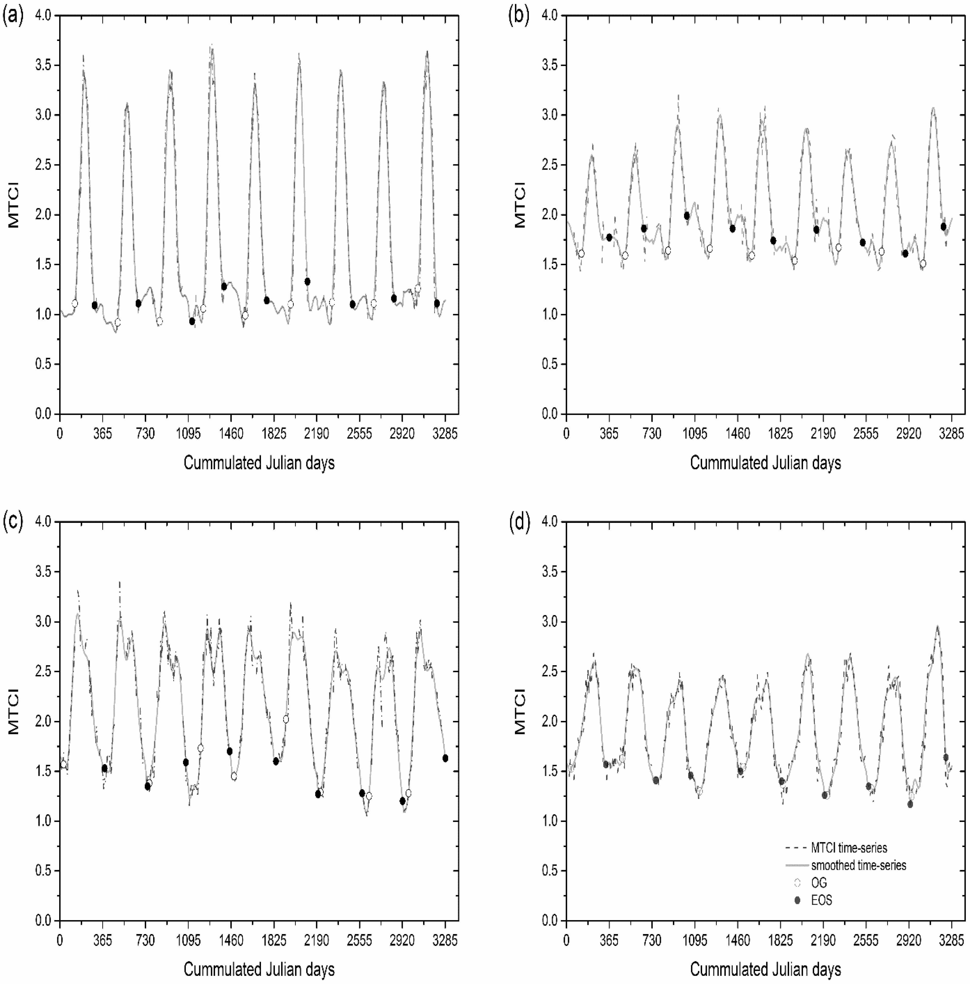
2.2. Phenology Estimates

The time-series MTCI data for every estimation period (i.e., year) used 1.5 years of data (from October in the previous year to the month of July in the next year) to estimate both the OG and EOS for every pixel. This length was used because the annual pattern spans across calendar years and hence complete information about LSP would not be obtained using single year data. The yearly values of OG and EOS were estimated for each image pixel of the study area using the methodology described in Dash, Jeganathan and Atkinson [18]. This methodology consists of two major procedures: data smoothing and extraction of phenological metrics.
The MERIS MTCI is a ratio of the difference in reflectance between band 10 and band 9 and the difference in reflectance between band 9 and band 8 of the MERIS standard band setting. Bands 10, 9 and 8 correspond to wavelengths 753.75 nm, 708.75 nm, and 681.25 nm, respectively. The MTCI time-series was smoothed using the Fourier method [45,46]. Although, there is a lack of general consensus regarding the robustness of smoothing methods and its performance can vary depending on data, Atkinson, et al. [47] showed that Fourier methods have a competitive performance when applied to MERIS MTCI data and require the specification of one parameter only, the number of harmonics for reconstruction. The first six Fourier components (mean + five harmonics) were used because they reproduced satisfactorily the original annual growth profile, obtaining a good fit between raw and smoothed MTCI time-series. Figure 1 shows some examples of raw MTCI and smoothed time-series as well as the extracted phenology metrics for different land cover types.
Figure 1. Inter-annual variation in MTCI values and phenology metrics for major natural vegetation types. (a) Broadleaved deciduous forests; (b) needleleaved evergreen forests; (c) grasslands; (d) shrublands.
Remotesensing 07 09390 g001
The first derivative (difference between one composite value and its immediate preceding neighbour) of MTCI time-series was computed to locate the annual maximum. This peak was defined as a point on the phenological profile where the curvature changes the sign before and after a negative and positive trend of five successive composites, respectively. Next, the derived data were searched backward and forward departing at the maximum annual peak to estimate the OG and EOS, respectively. OG was defined as a valley at the beginning of the growing season point (a change in derivative value from positive to negative) and EOS was defined as a valley point occurring at the decaying end of a phenology cycle (a change in derivative value from negative to positive) [18]. The searching function stops when a valley peak greater than one-fifth of the annual maximum peak is reached. The composite number identified during the phenology estimation procedure was then converted to Julian days, assigning the date of the last day of the composite period. Figure 1 shows some examples of MTCI time-series for different land covers and the estimated phenology metrics.
The length of the season was equal to the number of days between OG and EOS. The phenological information over homogeneous pixels was grouped and analysed in terms of each natural vegetation land cover and different biogeographical regions. The statistical significance of the differences in OG and EOS between different biogeographical regions was assessed through a two-tailed t-test. A median phenological map was produced from the 10 years of time-series data to characterise the spatial variation of phenology across Europe. The 10-year time-series analysed overcomes some limitations in the satellite sensor data quality for a specific year and minimises the inter-annual variation in LSP metrics.

3. Results

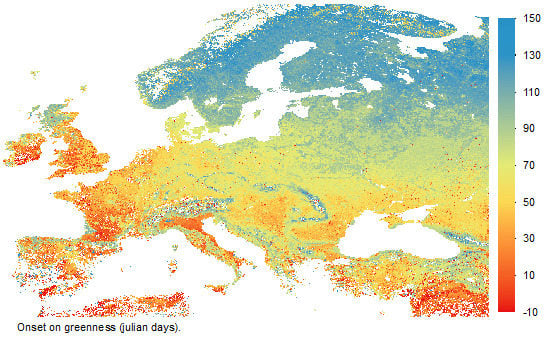
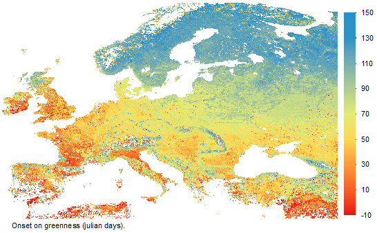
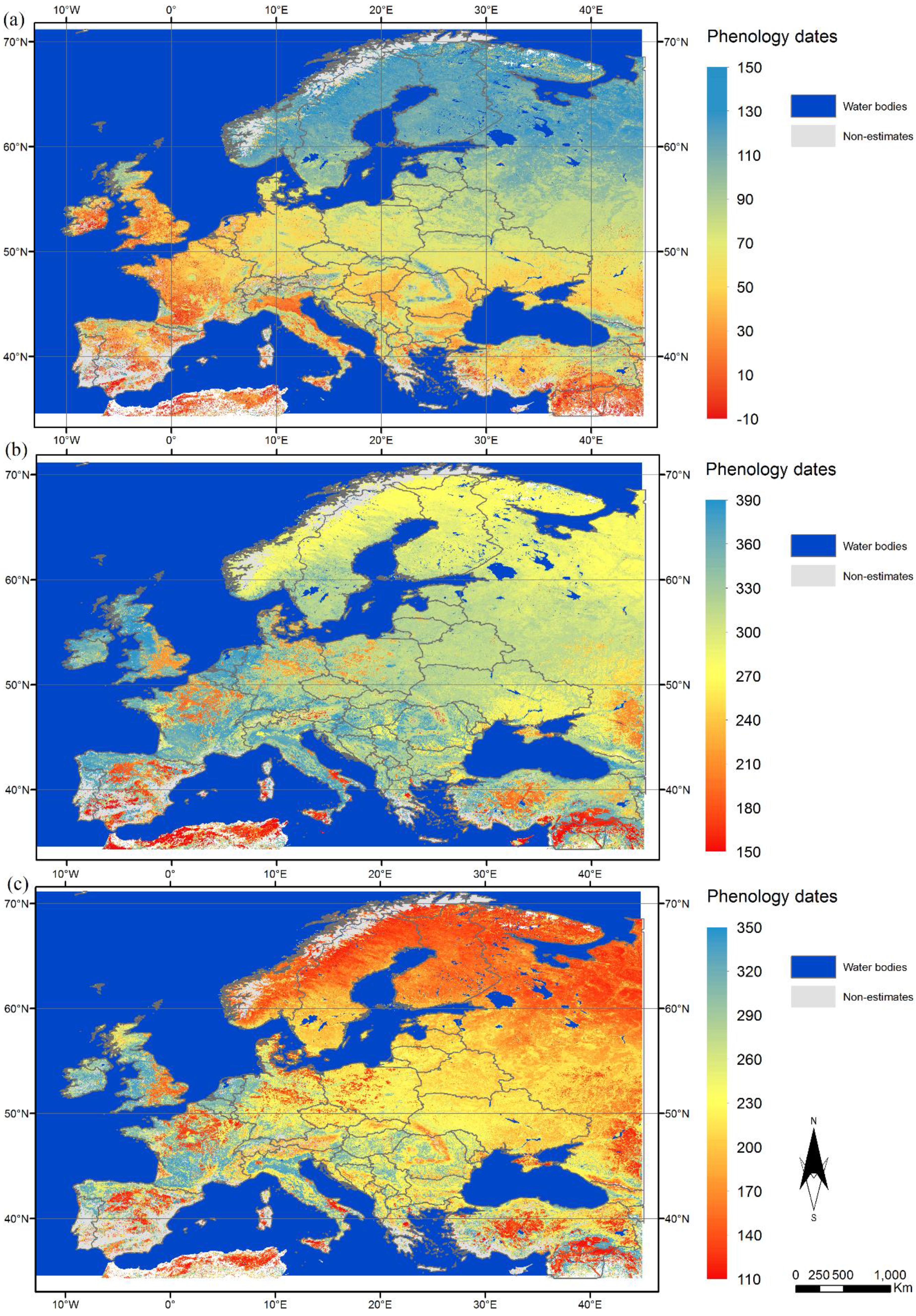
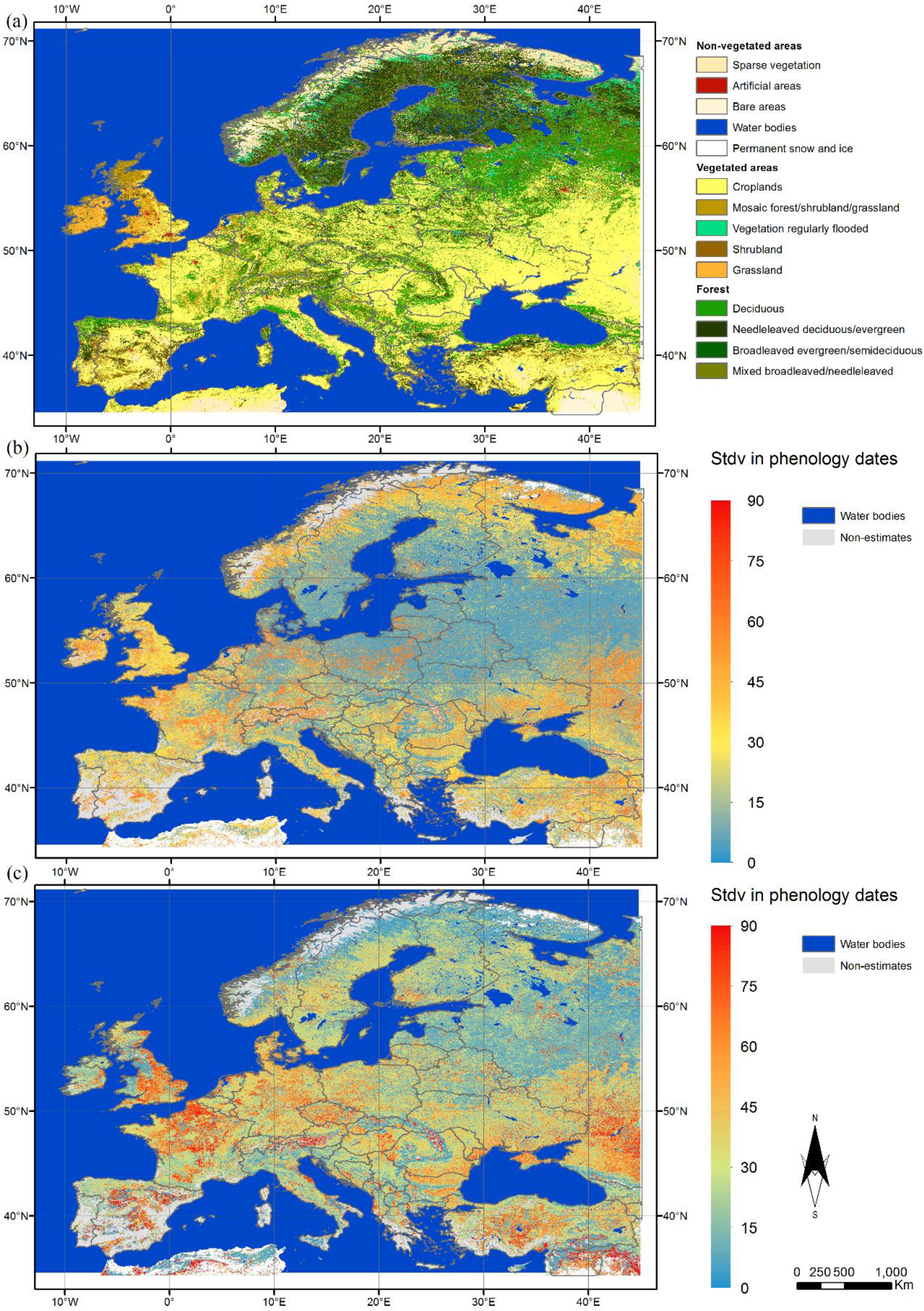
3.1. Spatial Variation in Phenological Metrics

Figure 2 shows the OG, EOS, and LS of the vegetation of the pan-European continent. OG dates are widely distributed from -10 days (approximately 21 December) to 150 days (30 May): later OG dates were observed at higher latitudes and vice versa. Earlier OG is associated mainly with rainfed croplands in the south of Europe and grasslands in Ireland and the southwest of England and Wales. On the other hand, later OG occurs in Fennoscandia and the north of Russia and in mountainous areas such as the Carpathians or the Caucasus. The progressive patterns in phenophases from low to high latitudes are attributed mainly to temperature variation [48], but also to the photoperiod and winter chilling requirements for some temperate tree species [5]. In terms of longitudinal variation, the OG of the Atlantic and Mediterranean basin regions is earlier than the OG of the Continental region. This is likely due to different vegetation responses to climatic conditions (i.e., temperature and precipitation) [39]. This large variability in phenophases could be explained not only by the difference in climatic conditions between coastal and interior continental regions, but also by the effect of changes in altitude associated with the mountain ridges.
The EOS dates range from 150 days (30 May) to 390 days (25 January), and their spatial distribution is generally the reverse of that of the OG dates for natural vegetation (Figure 2b). The later OG is generally coincident with a delayed EOS. However, this is only applicable to regions of natural or semi-natural vegetation, whereas cropland areas are characterised by earlier OG and EOS. Hence, regions with a later EOS exhibit longer length than regions with an earlier OG (Figure 2c). Note that there exist areas in Western Europe mainly associated with crops which present earlier dates for both OG and EOS.
Figure 2. Phenology maps of Europe. (a) Onset of greenness (OG); (b) end of senescence (EOS); (c) length of the season (LS).
Remotesensing 07 09390 g002
Figure 3. Standard deviation of phenology estimates. (a) Spatial distribution of different land cover types (DF); (b) onset of greenness (OG); (c) end of senescence (EOS).
Remotesensing 07 09390 g003
Figure 4. Boxplots showing the distribution of OG, EOS, and LS for each vegetation type and biogeographical region (box, interquartile range; horizontal line, median; vertical lines, minimum and maximum). Box plots are shown ordinally from earliest to latest date and resume the information about the timing of phenophases from 2003 to 2011. Map shows the spatial distribution of the European biogeographical regions delineated in the Habitats Directive (92/43/EEC). Colours in the map correspond to the colours of boxplots. Alpine (Alp), Anatolian (Ana), Black Sea (B. Sea), Continental (Cont), Mediterranean (Med), Panonian (Pan), and Steppic (Step).
Remotesensing 07 09390 g004
LS durations are given in Figure 2c. Shorter growing seasons (approximately three months) are associated with rainfed croplands in West Europe, and forests in boreal and mountainous areas. Maximum LS values (approximately one year) appear in the Atlantic basin associated with grasslands (see Figure 1d). Atzberger, Klisch, Mattiuzzi and Vuolo [41], Jeong, Ho, Gim and Brown [39], and Zhang, Tan and Yu [42], and Atzberger, Klisch, Mattiuzzi and Vuolo [41] found similar dates and patterns of variability for all phenophases. However, it should be noted that some differences can be attributed to the inclusion of crops in the present map.
The spatial distribution of spring phenophases (i.e., OG) is in agreement with the expected pattern of European classification of biogeographical regions and the GlobCover2009 land cover map. Interestingly, the spatial variability at a local scale (high frequency component) is determined by the type of land cover, whereas at a larger scale (low frequency component) the variability in phenophases matches the pattern of the biogeographical regions.
Figure 3 shows the standard deviation of LSP estimates over the 10-year period. The maximum deviation of EOS is larger than for OG in general terms (up to 90 days vs. 60 days, respectively). This could be due to either higher uncertainties in the estimates of autumn phenophases or a greater complexity of autumn phenology. All phenophases showed a similar spatial pattern in standard deviation which is driven mainly by land cover type. Rainfed crops in France and the United Kingdom experienced the greatest variability (mostly due to different crop types and management practices), followed also by crops in the Steppic biogeographic region (see Figure 4). Forests generally presented a very small variability, usually around five days. However, northern latitude forests presented a high variability in OG and a low variability in EOS. Although further research on this phenomenon in northern forests is required, it could be related to the photoperiod having a more important role in the senescence of northern forests (considering that the photoperiod is more stable in time than temperature).

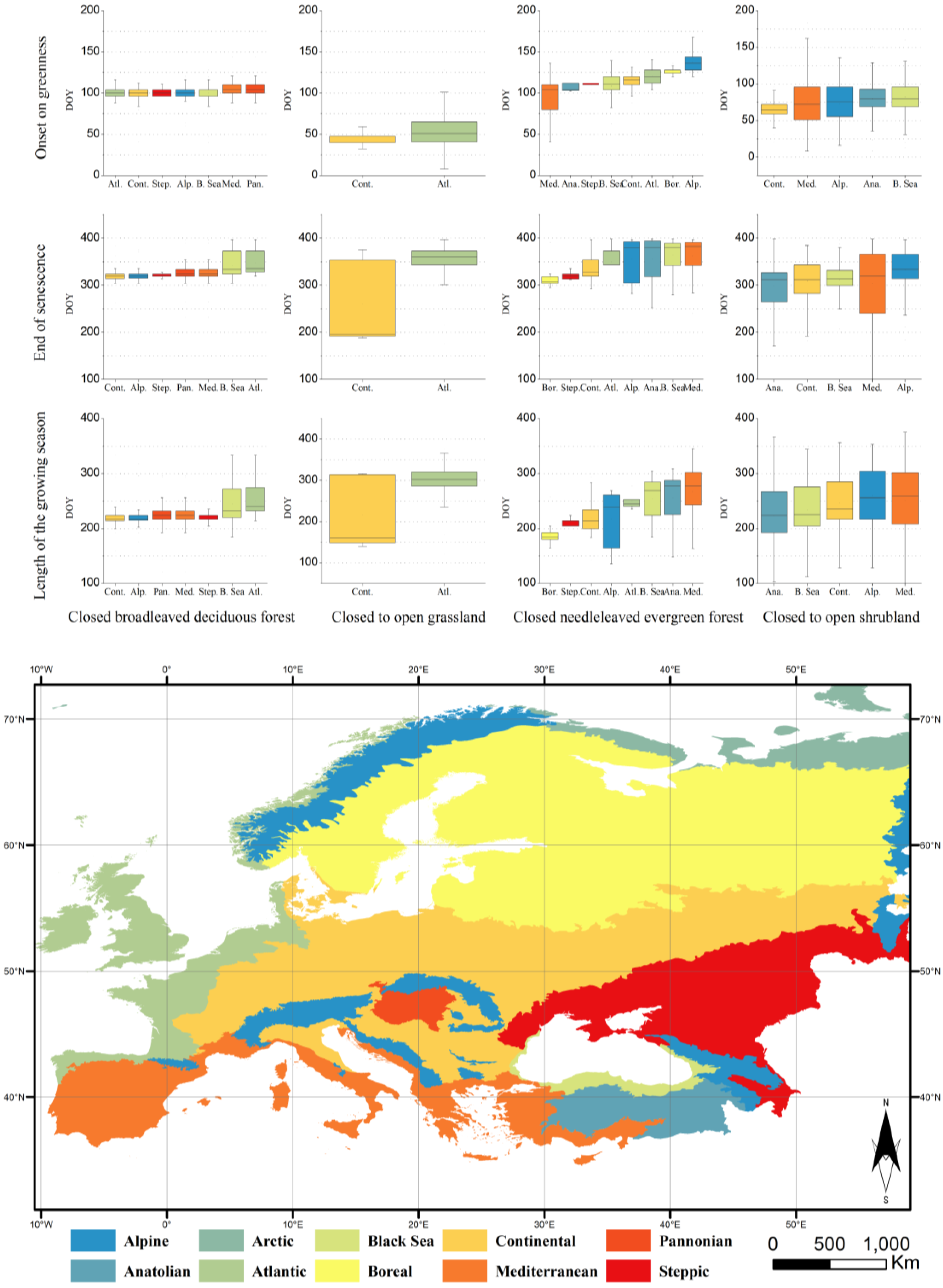
3.2. Characterisation of the Phenology of the Main Biogeographical Regions in Europe

LSP varies greatly over broad geographic gradients, according to climate zone and vegetation type [5]. Figure 4 shows the boxplot computed from homogeneous pixels of the four major natural vegetation types for the different European biogeographical regions. In general, grasslands present the earliest OG values, starting around the middle of February, followed by shrublands for which OG starts from the first week of March, deciduous trees the second week of April and needle-leaved evergreen forests from the same date as deciduous trees until mid-May, depending on the biogeographic region. A similar pattern can be observed for the end of senescence. However, there is greater variability within biogeographical regions. EOS is reached first by the continental grasslands around the middle of July, followed by Mediterranean evergreen forests at the end of August, shrublands from the second week of November, deciduous forests from the middle of November, and finally, evergreen forests, which can last until the end of the year. Regarding LS, Atlantic grasslands present the longest growing season, which is equal to 302 days, followed by the southern evergreen forests with LS over 250 days, and the shrublands and evergreen forests of the remaining biogeographical regions which vary between 184 (Boreal) and 245 (Atlantic) days. Shrublands and deciduous forests have similar growing season lengths (around 220 days) with slight variation depending on the biogeographical region.
Different levels of response to environmental drivers can be observed according to the vegetation type. For broadleaved deciduous forests and shrublands, the phenological variations are relatively stable in all regions, whereas needle-leaved evergreen forests or grasslands present greater variability between biogeographical regions and phenophases. The variation of OG of deciduous trees is grouped into two categories: Alpine regions and northern latitudes, such as Atlantic, Continental, and Steppe regions starting during the first week of April; and the southern biogeographical regions (Black Sea, Mediterranean, and Panonian), which start four days later. EOS dates are more diverse and ranged from 16 November for Alpine, Steppe, and Continental regions until 30 November and 2 December for the Black Sea and Atlantic Regions, respectively. In terms of LS, it can be observed that deciduous trees of regions with higher values of EOS produce slightly longer growing seasons (Atlantic and Black Sea), equal to 240 and 232 days, respectively, perhaps due to the oceanic influence keeping the temperature warmer for a relatively longer period. The timing of grasslands was estimated for the Atlantic and Continental regions only, as large homogeneous sites were not found for the remaining biogeographical regions. Grasslands present similar OG dates in both regions. However, there are important discrepancies regarding the EOS and LS times. Continental grasslands have a median EOS date equal to 196 Julian days (15 July), more than four months earlier than Atlantic grasslands (26 December). This results in a LS equal to five-and-a-half months for Continental grasslands against a LS of almost a year for Atlantic grasslands (11.8 months). Additionally, the variance in estimated EOS for Continental grasslands was significantly greater than for other categories. This can be due to the wide longitudinal range of the Continental region, but also to greater difficulty in estimating the autumnal phenophases in temperate regions [5].
Needle-leaved evergreen forests presents a latitudinally controlled phenological pattern which is mediated by the influence of relief. OG starts first in the south, around 14 April for Mediterranean and Anatolian regions, whereas the rest of the biogeographical regions are from one-to-four weeks delayed according to a latitudinal gradient. For Alpine evergreen forests, OG starts later than Boreal evergreen forests, with OG dates equal to 16 May and 6 May, respectively. This difference can be due to the influence of Alpine Tundra on the estimation of dates for the Alpine region. However, the EOS for Boreal evergreen forests is earlier than for any other biogeographical region (4 November), resulting in the shortest LS (184 days). The EOS for Steppe evergreen forests occurs 12 days later than for Boreal forests, followed by the Continental and Atlantic regions. The EOS for the Mediterranean, Anatolian, Black Sea, and Alpine regions spans the start of the calendar year occurring in mid-January. The LS of the three first regions mentioned before are quite similar, with LS values of nine months (277, 269, and 277 days, respectively). However, the length of the season in Alpine evergreen forests is shorter due to a much-delayed OG (7.8 months), which can be influenced by the timing of snowmelt and the photoperiod in the Alpine Tundra ecosystem [49].
Shrubland phenophases are quite similar between biogeographical regions, but have greater variation within a region. OG occurs from 4 March to 20 March, and EOS occurs from 8 November to 30 November. The LS for shrublands varies from 7.3 to 8.5 months. A clear latitudinal gradient could not be found for shrublands, presenting a high variance in phenophase date. This variation, especially in the Mediterranean region, could be associated to differences in elevation and precipitation, together with heterogeneity in the landscape [24].

4. Discussion

The present research was based on the estimation of the date of different land surface phenological events using MERIS MTCI time-series data, providing a description of how OG, EOS, and LS vary for major vegetation types across the main biogeographical regions of the pan-European continent. These results provide a description of European vegetation phenology for the last decade and provide a potential reference point against which to assess future climate impacts on vegetation growth cycles. The phenology maps obtained represent one of the most recent characterisations of vegetation phenology at the European continental scale, and were computed from MERIS MTCI data from 2002 to 2012 (the whole period of MERIS acquisitions) at a spatial resolution (1 km) finer than that of most previous studies.
The spatial distributions of the estimated OG, EOS, and LS follow the expected pattern of the European classification of biogeographical regions. Therefore, the obtained OG, EOS, and LS values are appropriate as a reference for analysing regional differences in the long-term variation in phenology cycles [39]. However, there were difficulties with obtaining homogeneous pixels for phenology estimation that can undermine the reliability of some of these estimates. On one hand, we used GlobCover2009, assuming that there were no changes in the natural vegetation land cover during this period. On the other hand, the heterogeneity of the landscape in certain regions due to the effects of relief or human factors made it difficult to identify sufficient pixels for some land cover types in certain regions. Apart from the issues related to pixel mixture, a mixed signal might also exist in a single land cover type due to multi-canopy layers [50,51]. In general, estimation for deciduous trees is more reliable than for other land-cover types, as they are well represented in all biogeographical regions and tend to form large patches of the same vegetation type, reducing the influence of mixed or border pixels. However, shrublands are usually more dispersed and less dense than deciduous forests and, therefore, are more likely to be associated with noisy (mixed) signals. This effect can be appreciated in the greater dispersion of the boxplots (Figure 4), although this greater variability can also be associated with greater relief. Most estimates of phenological dates (Figure 4), with the exception of continental grasslands and Atlantic and Steppe evergreen forests, were estimated from a large number of locations (hundreds of pure patches for every land cover type) within each biogeographical region. Additionally, it should be noted that all dates described in this study correspond to median values to minimize the effects described above. Table 2 and Table 3 show the statistical significance of the differences in the phenology dates of land covers in different biogeographical regions. Most biogeographical regions exhibited statistically significant differences for the dates of either OG or EOS (p-value < 0.05) and, therefore, different growing seasons, considering both timing and length. The differences in the autumn and spring phenology of shrublands between different biogeographical regions were significantly greater than those of other land covers. On the contrary, deciduous and evergreen forests exhibited greater similarities for OG or EOS dates in certain regions. More specifically, the average phenology of Alpine and Continental regions was not significantly different for deciduous forests. This is probably due to the broad similarity in their climatic pattern, in particular, the inter-annual pattern of temperature distribution. On the other hand, the Anatolian region was not found to be significantly different to most of the remaining regions, although the number of homogeneous deciduous tree samples (N = 15) might have limited the power of the t-test and, therefore, affected the interpretability of the results for this biogeographical region.
Table 2. p-values obtained from a two-tailed t-test between the OG of different biogeographical regions. Biogeographical regions with non-significant differences in both OG and EOS are given in bold.
Broadleaved Deciduous Forest
AlpineAnatolianBlack SeaContinentalMediterraneanPanonian
Anatolian0.067--
Black Sea0 *0.1--
Continental0.8080.0660 *--
Mediterranean0 *0.027 *0 *0 *--
Panonian0 *0.1050.6990 *0 *--
Steppic0.4670.0620 *0.5070 *0 *
Needleleaved Evergreen Forest
AlpineAnatolianBlack SeaContinentalMediterranean
Anatolian0 *--
Black Sea0 *0.03 *--
Continental0 *0 *0*--
Mediterranean0 *0.6910.001 *0 *--
Steppic0 *0.03 *0.8160.021 *0.002 *
Shrublands
AlpineAnatolianBlack SeaContinental
Anatolian0 *--
Black Sea0 *0 *--
Continental0 *0 *0 *--
Mediterranean0 *0 *0 *0 *
Grasslands
Continental
Atlantic0.826 *
* Statistically significant differences.
Comparisons of the satellite-derived phenological event dates in this study with those from previous studies could increase our understanding of the spatial patterns of vegetation phenology across Europe. Although, several studies of both LSP and ground phenology have been published in recent years focused on Europe or the Northern Hemisphere, most of them are related to phenology changes or trends across time, rather than the characterisation of phenological event dates. Apart from the scarce number of studies, there are some technical reasons that make a comparison challenging [42]. The determination of the timing of vegetation phenophases varies greatly according to different factors, including: (i) the methods applied to process the time-series (i.e., filtering or smoothing) [47,52]; (ii) the temporal base information estimate [16]; and (iii) the sensors and vegetation indices used [41,53]. Jeong, Ho, Gim and Brown [39], using NDVI time-series from different sensors, estimated the OG of temperate vegetation in the Northern Hemisphere from 21 March to 20 May, and the EOS from 17 September to 26 November. Although the same latitudinal and longitudinal pattern can be observed (Figure 2), there are significant differences in terms of their study design and data used that make a comparison between the absolute dates difficult. The latitudinal range of the mentioned study is narrower, as they did not consider crops, which are present in many areas of southern Europe. Based on estimation for homogeneous pixels only (Figure 4), our findings revealed a different timing for the phenological events: the earliest OG occurred for the Atlantic grasslands around 17 February and the latest for Alpine evergreen forests on 16 May. EOS ranged from 5 July (Continental grasslands) to16 January (Mediterranean evergreen forests). On the other hand, comparing our results to the dates for deciduous trees from the International Phenological Gardens (IPG) dataset reported by Chmielewski and Rötzer [54], we obtained an earlier pattern for spring phenology and a delayed pattern for autumn. Specifically, LSP, OG, and EOS occurred 11 days earlier and 30 days later than the start and end of the season of IPG trees, respectively. This has been reported as expected by different studies that compare LSP and ground phenology [16]. However, it should be noted that the study period of the cited study and the definition of start and end of the season are different.
Table 3. p-values obtained from a two-tailed t-test between the OG of different biogeographical regions. Significant differences are highlighted with an asterisk. Biogeographical regions with non-significant differences in both OG and EOS are given in bold.
Broadleaved Deciduous Forest
AlpineAnatolianBlack SeaContinentalMediterraneanPanonian
Anatolian0.271--
Black Sea0 *0.137--
Continental0.3240.250 *--
Mediterranean0 *0.9990 *0 *--
Panonian0.1680.3640 *0.0860 *--
Steppic0.021 *0.3660 *0.001 *0 *0.949
Needleleaved Evergreen Forest
AlpineAnatolianBlack SeaContinentalMediterranean
Anatolian0.836--
Black Sea0.1540.202--
Continental0.048 *0.3280 *--
Mediterranean0 *0 *0 *0 *--
Steppic0 *0.018 *0 *0.006 *0 *
Shrublands
AlpineAnatolianBlack SeaContinental
Alpine--
Anatolian0 *--
Black Sea0 *0 *--
Continental0 *0 *0.001 *--
Mediterranean0 *0 *0.380 *
Grasslands
Continental
Atlantic0 *
* Statistically significant differences.

5. Conclusions

MERIS MTCI time-series were used to spatially characterise the phenology of the pan-European continent, and this phenology was analysed by main vegetation type and biogeographical region. Spatial variability in OG, EOS, and LS was determined by analysing homogeneous groups of vegetated pixels, defined in terms of vegetation type and biogeographical region. In line with expectations, incremental latitudinal variation was observed for OG, whereas the opposite pattern was found for EOS, when considering natural vegetation. However, this latitudinal gradient was interrupted in mountainous regions. In terms of longitude, coastal regions experienced an earlier OG and more delayed EOS than interior regions. Statistically significant differences existed between biogeographical regions in terms of the dates of both OG and EOS for all land cover types considered in this study.
The phenology maps produced here represent one of the most comprehensive and recent assessments of the land surface phenology of continental Europe at a 1 km spatial resolution. The spatial variability of phenology can be used for tuning models of carbon emissions and can play an important role in monitoring programmes for the management of natural vegetation. Further research is needed to study and understand the main drivers of LSP in Europe among different land covers and biogeographic regions.

Acknowledgments

The first author is a Marie Curie Grant holder (Ref. FP7-PEOPLE-2012-IEF- 331667). The authors are grateful for the financial support given by the European Commission under the 7th Framework Programme, the Spanish MINECO (project BIA2013-43462-P), and Junta de Andalucía (Group RNM122). PMA is grateful to the University of Utrecht for supporting him with The Belle van Zuylen Chair.

Author Contributions

Victor F. Rodriguez-Galiano, Jadunandan Dash and Peter M. Atkinson conceived and designed the experiments; Victor F. Rodriguez-Galiano performed the experiments; Victor F. Rodriguez-Galiano analysed the data; Jadunandan Dash contributed analysis tools; Victor F. Rodriguez-Galiano drafted the paper. All authors contributed to the final paper.

Conflicts of Interest

The authors declare no conflict of interest.

References

  1. Parmesan, C.; Yohe, G. A globally coherent fingerprint of climate change impacts across natural systems. Nature 2003, 421, 37–42. [Google Scholar] [CrossRef] [PubMed]
  2. Menzel, A.; Sparks, T.H.; Estrella, N.; Koch, E.; Aaasa, A.; Ahas, R.; Alm-Kübler, K.; Bissolli, P.; Braslavská, O.; Briede, A.; et al. European phenological response to climate change matches the warming pattern. Glob. Change Biol. 2006, 12, 1969–1976. [Google Scholar] [CrossRef]
  3. Wolkovich, E.M.; Cook, B.I.; Allen, J.M.; Crimmins, T.M.; Betancourt, J.L.; Travers, S.E.; Pau, S.; Regetz, J.; Davies, T.J.; Kraft, N.J.B.; et al. Warming experiments underpredict plant phenological responses to climate change. Nature 2012, 485, 494–497. [Google Scholar] [CrossRef] [PubMed]
  4. Sobrino, J.A.; Julien, Y.; Morales, L. Changes in vegetation spring dates in the second half of the twentieth century. Int. J. Remote Sens. 2011, 32, 5247–5265. [Google Scholar] [CrossRef]
  5. Richardson, A.D.; Keenan, T.F.; Migliavacca, M.; Ryu, Y.; Sonnentag, O.; Toomey, M. Climate change, phenology, and phenological control of vegetation feedbacks to the climate system. Agric. For. Meteorol. 2013, 169, 156–173. [Google Scholar] [CrossRef]
  6. Menzel, A. Phenology: Its importance to the global change community. Clim. Change 2002, 54, 379–385. [Google Scholar] [CrossRef]
  7. Betts, R.A. Offset of the potential carbon sink from boreal forestation by decreases in surface albedo. Nature 2000, 408, 187–190. [Google Scholar] [CrossRef] [PubMed]
  8. Klosterman, S.T.; Hufkens, K.; Gray, J.M.; Melaas, E.; Sonnentag, O.; Lavine, I.; Mitchell, L.; Norman, R.; Friedl, M.A.; Richardson, A.D. Evaluating remote sensing of deciduous forest phenology at multiple spatial scales using Phenocam imagery. Biogeosciences Discuss. 2014, 11, 2305–2342. [Google Scholar] [CrossRef]
  9. Kirbyshire, A.L.; Bigg, G.R. Is the onset of the English summer advancing? Clim. Change 2010, 100, 419–431. [Google Scholar] [CrossRef]
  10. Fitter, A.H.; Fitter, R.S.R. Rapid changes in flowering time in British plants. Science 2002, 296, 1689–1691. [Google Scholar] [CrossRef] [PubMed]
  11. Menzel, A. Trends in phenological phases in Europe between 1951 and 1996. Int. J. Biometeorol. 2000, 44, 76–81. [Google Scholar] [CrossRef] [PubMed]
  12. Roetzer, T.; Wittenzeller, M.; Haeckel, H.; Nekovar, J. Phenology in Central Europe differences and trends of spring phenophases in urban and rural areas. Int. J. Biometeorol. 2000, 44, 60–66. [Google Scholar] [CrossRef] [PubMed]
  13. Defila, C.; Clot, B. Phytophenological trends in Switzerland. Int. J. Biometeorol. 2001, 45, 203–207. [Google Scholar] [CrossRef] [PubMed]
  14. Ahas, R.; Aasa, R.; Menzel, A.; Fedotova, V.G.; Scheifinger, H. Changes in European spring phenology. Int. J. Climatol. 2002, 22, 1727–1738. [Google Scholar] [CrossRef]
  15. Studer, S.; Stöckli, R.; Appenzeller, C.; Vidale, P.L. A comparative study of satellite and ground-based phenology. Int. J. Biometeorol. 2007, 51, 405–414. [Google Scholar] [CrossRef] [PubMed]
  16. White, M.A.; de Beurs, K.M.; Didan, K.; Inouye, D.W.; Richardson, A.D.; Jensen, O.P.; O’Keefe, J.; Zhang, G.; Nemani, R.R.; van Leeuwen, W.J.D.; et al. Intercomparison, interpretation, and assessment of spring phenology in North America estimated from remote sensing for 1982–2006. Glob. Change Biol. 2009, 15, 2335–2359. [Google Scholar] [CrossRef]
  17. Jeganathan, C.; Dash, J.; Atkinson, P. Characterising the spatial pattern of phenology for the tropical vegetation of India using multi-temporal MERIS chlorophyll data. Landsc. Ecol. 2010, 25, 1125–1141. [Google Scholar] [CrossRef]
  18. Dash, J.; Jeganathan, C.; Atkinson, P.M. The use of MERIS terrestrial chlorophyll index to study spatio-temporal variation in vegetation phenology over India. Remote Sens. Environ. 2010, 114, 1388–1402. [Google Scholar] [CrossRef]
  19. Reed, B.C.; Brown, J.F.; VanderZee, D.; Loveland, T.R.; Merchant, J.W.; Ohlen, D.O. Measuring phenological variability from satellite imagery. J. Veg. Sci. 1994, 5, 703–714. [Google Scholar] [CrossRef]
  20. Maignan, F.; Bréon, F.M.; Vermote, E.; Ciais, P.; Viovy, N. Mild winter and spring 2007 over western Europe led to a widespread early vegetation onset. Geophys. Res. Lett. 2008, 35. [Google Scholar] [CrossRef]
  21. Dash, J.; Curran, P.J. Evaluation of the MERIS terrestrial chlorophyll index (MTCI). Adv. Space Res. 2007, 39, 100–104. [Google Scholar] [CrossRef]
  22. Beck, P.S.A.; Atzberger, C.; Høgda, K.A.; Johansen, B.; Skidmore, A.K. Improved monitoring of vegetation dynamics at very high latitudes: A new method using MODIS NDVI. Remote Sens. Environ. 2006, 100, 321–334. [Google Scholar] [CrossRef]
  23. O’Connor, B.; Dwyer, E.; Cawkwell, F.; Eklundh, L. Spatio-temporal patterns in vegetation start of season across the island of Ireland using the MERIS global vegetation index. ISPRS J. Photogramm. Remote Sens. 2012, 68, 79–94. [Google Scholar] [CrossRef]
  24. Delbart, N.; Picard, G.; Le Toans, T.; Kergoat, L.; Quegan, S.; Woodward, I.; Dye, D.; Fedotova, V. Spring phenology in Boreal Eurasia over a nearly century time scale. Glob. Change Biol. 2008, 14, 603–614. [Google Scholar] [CrossRef]
  25. Hamunyela, E.; Verbesselt, J.; Roerink, G.; Herold, M. Trends in spring phenology of western European deciduous forests. Remote Sens. 2013, 5, 6159–6179. [Google Scholar] [CrossRef]
  26. Han, Q.; Luo, G.; Li, C. Remote sensing-based quantification of spatial variation in canopy phenology of four dominant tree species in Europe. J. Appl. Remote Sens. 2013, 7. [Google Scholar] [CrossRef]
  27. Klisch, A.; Atzberger, C.; Luminari, L. Satellite-based drought monitoring in Kenya in an operational setting. ISPRS Int. Arch. Photogramm. Remote Sens. Spat. Inf. Sci. 2015, 2015, 433–439. [Google Scholar] [CrossRef]
  28. Rodriguez-Galiano, V.; Dash, J.; Atkinson, P.M. Inter-comparison of satellite sensor land surface phenology and ground phenology in Europe. Geophys. Res. Lett. 2015, 42, 2253–2260. [Google Scholar] [CrossRef]
  29. Myneni, R.B.; Keeling, C.D.; Tucker, C.J.; Asrar, G.; Nemani, R.R. Increased plant growth in the northern high latitudes from 1981 to 1991. Nature 1997, 386, 698–702. [Google Scholar] [CrossRef]
  30. Tucker, C.J.; Slayback, D.A.; Pinzon, J.E.; Los, S.O.; Myneni, R.B.; Taylor, M.G. Higher northern latitude normalized difference vegetation index and growing season trends from 1982 to 1999. Int. J. Biometeorol. 2001, 45, 184–190. [Google Scholar] [CrossRef] [PubMed]
  31. Zhou, L.M.; Tucker, C.J.; Kaufmann, R.K.; Slayback, D.; Shabanov, N.V.; Myneni, R.B. Variations in northern vegetation activity inferred from satellite data of vegetation index during 1981 to 1999. J. Geophys. Res. Atmos. 2001, 106, 20069–20083. [Google Scholar] [CrossRef]
  32. Stockli, R.; Vidale, P.L. European plant phenology and climate as seen in a 20-year AVHRR land-surface parameter dataset. Int. J. Remote Sens. 2004, 25, 3303–3330. [Google Scholar] [CrossRef]
  33. Tateishi, R.; Ebata, M. Analysis of phenological change patterns using 1982–2000 advanced very high resolution radiometer (AVHRR) data. Int. J. Remote Sens. 2004, 25, 2287–2300. [Google Scholar] [CrossRef]
  34. Karlsen, S.R.; Solheim, I.; Beck, P.S.A.; Hogda, K.A.; Wielgolaski, F.E.; Tommervik, H. Variability of the start of the growing season in Fennoscandia, 1982–2002. Int. J. Biometeorol. 2007, 51, 513–524. [Google Scholar] [CrossRef] [PubMed]
  35. Maignan, F.; Bréon, F.M.; Bacour, C.; Demarty, J.; Poirson, A. Interannual vegetation phenology estimates from global AVHRR measurements. Comparison with in situ data and applications. Remote Sens. Environ. 2008, 112, 496–505. [Google Scholar] [CrossRef]
  36. Julien, Y.; Sobrino, J.A. Global land surface phenology trends from GIMMS database. Int. J. Remote Sens. 2009, 30, 3495–3513. [Google Scholar] [CrossRef]
  37. De Beurs, K.M.; Henebry, G.M. A land surface phenology assessment of the Northern Polar regions using MODIS reflectance time series. Can. J. Remote Sens. 2010, 36, S87–S110. [Google Scholar] [CrossRef]
  38. Hogda, K.A.; Tommervik, H.; Karlsen, S.R. Trends in the start of the growing season in Fennoscandia 1982–2011. Remote Sens. 2013, 5, 4304–4318. [Google Scholar] [CrossRef]
  39. Jeong, S.-J.; Ho, C.-H.; Gim, H.-J.; Brown, M.E. Phenology shifts at start vs. End of growing season in temperate vegetation over the Northern Hemisphere for the period 1982–2008. Glob. Change Biol. 2011, 17, 2385–2399. [Google Scholar] [CrossRef]
  40. Ivits, E.; Cherlet, M.; Tóth, G.; Sommer, S.; Mehl, W.; Vogt, J.; Micale, F. Combining satellite derived phenology with climate data for climate change impact assessment. Glob. Planet. Change 2012, 88–89, 85–97. [Google Scholar] [CrossRef]
  41. Atzberger, C.; Klisch, A.; Mattiuzzi, M.; Vuolo, F. Phenological metrics derived over the European continent from NDVI3G data and MODIS time series. Remote Sens. 2013, 6, 257–284. [Google Scholar] [CrossRef]
  42. Zhang, X.; Tan, B.; Yu, Y. Interannual variations and trends in global land surface phenology derived from enhanced vegetation index during 1982–2010. Int. J. Biometeorol. 2014, 58, 1–18. [Google Scholar] [CrossRef]
  43. Defourny, P.; Vancutsem, C.; Bicheron, P.; Brockmann, C.; Nino, F.; Schouten, L.; Leroy, M. Globcover: A 300 m Global Land Cover Product for 2005 Using Envisat MERIS Time Series. Available online: http://dup.esrin.esa.int/files/131-176-131-25_2007510152728.pdf (accessed on 21 July 2015).
  44. Bicheron, P.; Amberg, V.; Bourg, L.; Petit, D.; Huc, M.; Miras, B.; Brockmann, C.; Hagolle, O.; Delwart, S.; Ranera, F.; et al. Geolocation assessment of MERIS globcover orthorectified products. IEEE Trans. Geosci. Remote Sens. 2011, 49, 2972–2982. [Google Scholar] [CrossRef] [Green Version]
  45. Verhoef, W.; Menenti, M.; Azzali, S. Cover a colour composite of NOAA-AVHRR-NDVI based on time series analysis (1981–1992). Int. J. Remote Sens. 1996, 17, 231–235. [Google Scholar] [CrossRef]
  46. Roerink, G.J.; Menenti, M.; Verhoef, W. Reconstructing cloudfree NDVI composites using fourier analysis of time series. Int. J. Remote Sens. 2000, 21, 1911–1917. [Google Scholar] [CrossRef]
  47. Atkinson, P.M.; Jeganathan, C.; Dash, J.; Atzberger, C. Inter-comparison of four models for smoothing satellite sensor time-series data to estimate vegetation phenology. Remote Sens. Environ. 2012, 123, 400–417. [Google Scholar] [CrossRef]
  48. Schwartz, M.D.; Ahas, R.; Aasa, A. Onset of spring starting earlier across the Northern Hemisphere. Glob. Change Biol. 2006, 12, 343–351. [Google Scholar] [CrossRef]
  49. Delbart, N.; Picard, G.; Le Toan, T.; Kergoat, L.; Quegan, S.; Woodward, I.; Dye, D.; Fedotova, V. Spring phenology in Boreal Eurasia over a nearly century time scale. Glob. Change Biol. 2008, 14, 603–614. [Google Scholar] [CrossRef]
  50. Ryu, Y.; Lee, G.; Jeon, S.; Song, Y.; Kimm, H. Monitoring multi-layer canopy spring phenology of temperate deciduous and evergreen forests using low-cost spectral sensors. Remote Sens. Environ. 2014, 149, 227–238. [Google Scholar] [CrossRef]
  51. Karnieli, A. Natural vegetation phenology assessment by ground spectral measurements in two semi-arid environments. Int. J. Biometeorol. 2003, 47, 179–187. [Google Scholar] [CrossRef] [PubMed]
  52. Atzberger, C.; Eilers, P.H.C. Evaluating the effectiveness of smoothing algorithms in the absence of ground reference measurements. Int. J. Remote Sens. 2011, 32, 3689–3709. [Google Scholar] [CrossRef]
  53. Seixas, J.; Carvalhais, N.; Nunes, C.; Benali, A. Comparative analysis of MODIS-FAPAR and MERIS–MGVI datasets: Potential impacts on ecosystem modeling. Remote Sens. Environ. 2009, 113, 2547–2559. [Google Scholar] [CrossRef]
  54. Chmielewski, F.-M.; Rötzer, T. Response of tree phenology to climate change across Europe. Agric. For. Meteorol. 2001, 108, 101–112. [Google Scholar] [CrossRef]

