SPOT-4 (Take 5): Simulation of Sentinel-2 Time Series on 45 Large Sites

Abstract

This paper presents the SPOT-4 (Take 5) experiment, aimed at providing time series of optical images simulating the repetitivity, the resolution and the large swath of Sentinel-2 images. The aim was to help users set up and test their applications and methods, before Sentinel-2 mission data become available. In 2016, when both Sentinel-2 satellites are operational, and for at least fifteen years, users will have access to high resolution time series of images systematically acquired every five days, over the whole Earth land surfaces. Thanks to Sentinel-2’s high revisit frequency, a given surface should be observed without clouds at least once a month, except in the most cloudy periods and regions. In 2013, the Centre National d’Etudes Spatiales (CNES) lowered the orbit altitude of SPOT-4, to place it on a five-day repeat cycle orbit for a duration of five months. This experiment started on 31 January 2013 and lasted until 19 June 2013. SPOT-4 images were acquired every fifth day, over 45 sites scattered in nearly all continents and covering very diverse biomes for various applications. Two ortho-rectified products were delivered for each acquired image that was not fully cloudy, expressed either as top of atmosphere reflectance (Level 1C) or as surface reflectance (Level 2A). An extensive validation campaign was held to check the performances of these products with regard to the multi-temporal registration, the quality of cloud masks, the accuracy of aerosol optical thickness estimates and the quality of surface reflectances. Despite high a priori geo-location errors, it was possible to register the images with an accuracy better than 0.5 pixels in the large majority of cases. Despite the lack of a blue band on the SPOT-4 satellite, the cloud and shadow detection yielded good results, while the aerosol optical thickness was measured with a root mean square error better than 0.06. The surface reflectances after atmospheric correction were compared with in situ data and other satellite data showing little bias and the standard deviation of surface reflectance errors in the range (0.01–0.02). The Take 5 experiment is being repeated in 2015 with the SPOT-5 satellite with an enhanced resolution.

1. Introduction

Sentinel-2 is one of the satellite missions of the European Space Agency (ESA) developed in the framework of the European Union Copernicus program [1]. This optical remote sensing mission will gather the following features for the first time for a space mission:

• Resolution: 10 m, 20 m or 60 m, depending on the spectral band
• Coverage: all lands systematically observed, with a field of view of 290 km
• Revisit: each land pixel observed every fifth day with a constant viewing angle
• Spectral: 13 spectral bands in the visible, near infrared (NIR) and short wave infrared (SWIR) domains, among which three bands are dedicated to atmospheric correction, a blue band for aerosol and cloud detection, a water vapor band in the NIR and a band to detect high clouds in the SWIR.

To obtain these features, the Sentinel-2 mission will rely on two satellites, the first of which was launched in June 2015, and the second is expected in 2016. Usually, when the development of a new satellite mission starts, space agencies set up a preparatory program [2,3] to provide simulated data to future users. Thanks to that, users can get ready to use the mission data as soon as they are available, after the satellite and ground segment commissioning phases. This is often done using aerial acquisitions that provide simulations of the future images, but in the case of ESA’s Sentinel-2 program, this task is complex, because the main new feature of the mission is its capacity to acquire time series with a frequent revisit. Such a characteristic is not easily obtained with aerial acquisitions.

Hence, before the SPOT-4 (Take 5) experiment, the existing datasets only fulfilled two of the four main features described above:

• ESA provided simulated data resulting from aerial acquisitions, with the 13 spectral bands at the proper resolutions, but with a very small coverage and no repetitivity;
• CNES and Centre d’Etudes Spatiales de la Biospher̀e (CESBIO) provided Formosat-2 satellite time series with the appropriate repetitivity at a constant viewing angle and 8-m resolution, but with a small coverage ($24\times 24$ km${}^2$) and only four bands (and no SWIR) [4];
• Landsat data with adequate coverage and good spectral richness could also be used; however, the repetitivity is much lower (16 days), and the resolution is only 30 m;
• SPOT and RapidEye imagery have the necessary resolution and may cover large sites, but do not provide repetitivity with constant angles and only have four or five bands, respectively;

To cope with this problem, the SPOT-4 (Take 5) experiment was proposed by the CESBIO and implemented by CNES. It consisted in lowering the SPOT-4 altitude by 2 km to put it on a five-day repeat cycle orbit. From this orbit, it was possible to acquire time series of images with the following characteristics:

• Resolution: 20 m
• Coverage: 45 sites, observed with a field of view of 60 to 120 km using both SPOT-4 HRVIR (Haute Résolution Visible et InfraRouge)instruments. By merging observations from adjacent orbits, it was possible to obtain 200 km-wide sites.
• Revisit: five days with constant viewing angles.
• Spectral: four bands, including a SWIR band (green, red, NIR and SWIR)

The SPOT-4 (Take 5) experiment was formally decided by CNES on 11 December 2012; the satellite rallied the five day cycle orbit at 819 km on 29 January 2013, and the first images were taken two days after, on 31 January. The experiment lasted until 19 June 2013. During this period, each of the 45 selected sites (see the next section for a description of the sites) was observed every fifth day, a total of 28 times. Finally, SPOT-4 was de-orbited and switched off after the end of the experiment, in June 2013.

The dataset is aimed at helping users to learn to process the information brought by the unique set of Sentinel-2 features, among which the most unusual is the availability of repetitive observations under constant viewing angles and at a high spatial resolution. Development of new techniques, methods and applications is needed to take full advantage of Sentinel-2 time series, and SPOT-4 (Take 5) data can be used to test these new ideas. Two products were delivered to the users, for which we used the nomenclature defined for Sentinel-2 [1]: a Level 1C product providing ortho-rectified images expressed in top of atmosphere reflectances and a Level 2A product providing the same ortho-rectified images, but expressed in surface reflectance after atmospheric correction and provided with cloud, cloud shadow, water and snow masks.

Together with the production of SPOT-4 (Take 5) products, an intensive validation campaign was set up to test the accuracy of Level 1C and Level 2A products in many aspects, such as ortho-rectification, cloud detection, atmospheric correction or measurement of biophysical variables, such as LAI and fAPAR. This paper describes the dataset and its processing, presents the validation results and summarizes a few lessons learned from the experiment.

2. List of Available Sites

The selection of the sites was split into two parts: about half of the images were attributed to French institutions, while the other half were attributed to international partners (see Table 1):

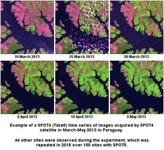
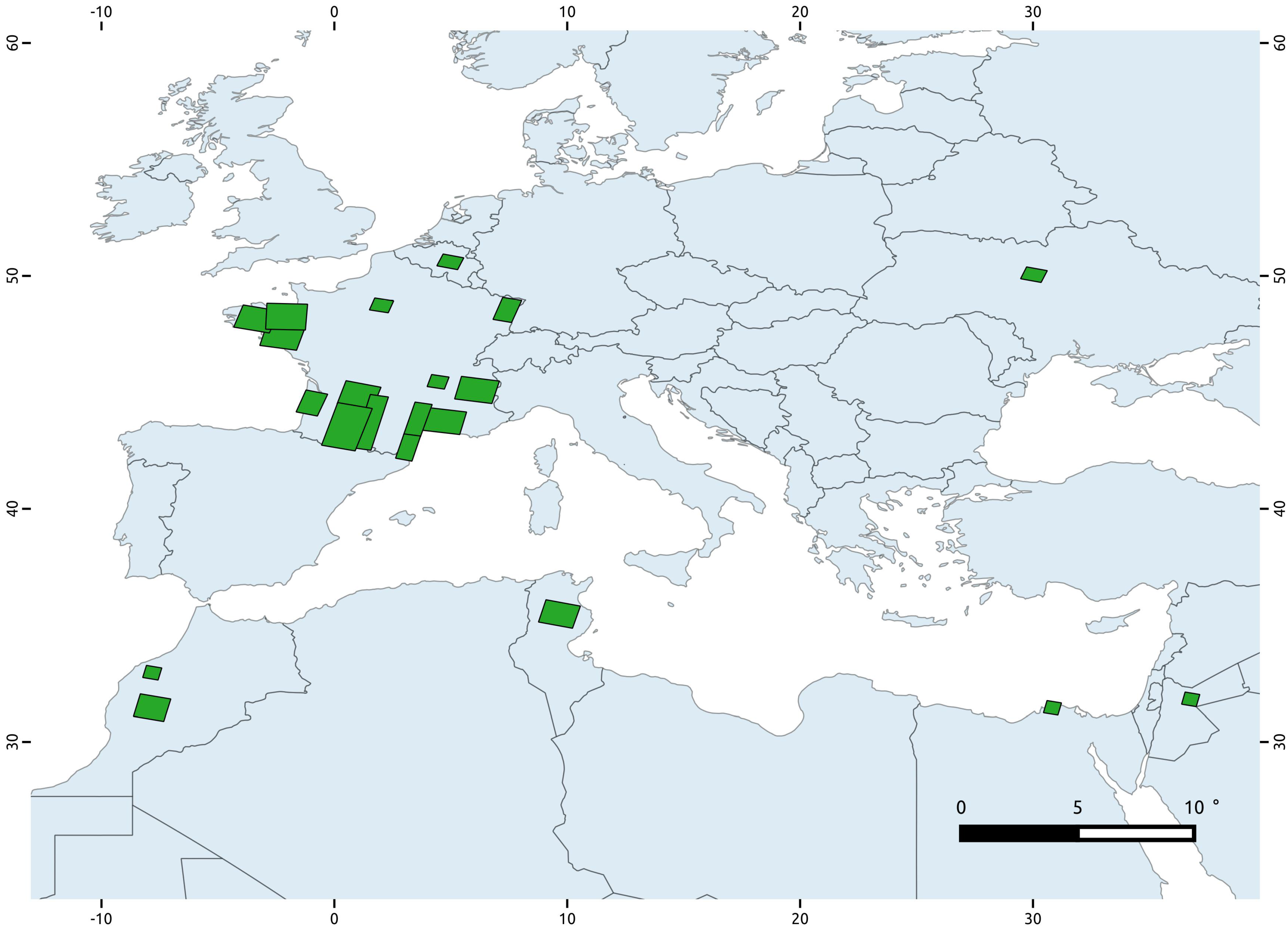
• In France, it was decided to issue a call for site proposals to the French scientific community and to French public institutions. Twenty site proposals were received, and sixteen sites were finally chosen, 11 of which were in France. Some larger sites were composed of several images, as shown in Figure 1.
• At the international level, the schedule was too short to issue a call for proposals, and we contacted only space agencies with which collaborations were already in place in the optical remote sensing domain. The European Space Agency (ESA), the National Aeronautics and Space Administration (NASA), the European Commission Joint Research Center (JRC) and the Canadian Center for Remote Sensing (CCRS) joined the experiment, selected several sites (see Table 1) and shared a part of the cost.

Figure 1. The green polygons show the situation of the sites in Europe and North Africa.

Figure 1. The green polygons show the situation of the sites in Europe and North Africa.

Table 1. List of SPOT-4 (Take 5) sites.

Site	Longitude	Latitude	Agency	Size (km${}^2$)	AeroNet Site
ALPES	5.769	45.153	CNES	$110\times 110$	-
ALSACE	7.4658	48.5539	CNES	$60\times 110$	-
AQUITAINE	−0.953	44.535	CNES	$60\times 110$	Arcachon
ARDECHE	4.484	45.472	CNES	$60\times 60$	-
LOIRE	−2.595	47.45	CNES	$110\times 110$	-
BRETAGNE	–3.718	48.217	CNES	$110\times 110$	-
RENNES	−2.05	48.27	CNES	$110\times 110$	-
CHINA (1)	115.993	29.32	CNES	$110\times 110$	-
CONGO (1)	16.898	3.092	CNES	$110\times 60$	-
MADAGASCAR	46.674	−19.582	CNES	$110\times 110$	-
MOROCCO(1)	−8.152	31.518	CNES	$110\times 110$	-
PROVENCE	4.322	43.803	CNES	$110\times 110$	Carpentras, le Frioul
LANGUEDOC	3.36	43.3768	CNES	$60\times 170$	-
ROUSSILLON	3.15	42.6	CNES	$60\times 170$	-
SUDMIPY E	1.5701	43.7292	CNES	$60\times 300$	Seysses, Le Fauga
SUDMIPY O	0.201	43.651	CNES	$110\times 240$	-
DORDOGNE	1.1	44.9	CNES	$110\times 110$	-
TUNISIA	9.342	35.583	CNES	$110\times 110$	Ben Salem
VERSAILLES	2.0024	48.7595	CNES	$60\times 60$	-
CCRS	−111.65	57.0208	CCRS	$60\times 60$	-
ARGENTINA	−59.577	−34.196	ESA	$60\times 60$	-
BELGIUM	4.985	50.64	ESA	$60\times 60$	Bruxelles
CHESAPEAKE	−76.115	37.7926	ESA	$60\times 60$	Wallops
CHINA (2)	116.569	36.831	ESA	$60\times 60$	-
EGYPT	30.826	31.484	ESA	$60\times 60$	-
ETHIOPIA	37.8571	9.1291	ESA	$60\times 60$	-
GABON	10.8063	0.3755	ESA	$60\times 60$	-
JORDAN	36.825	31.831	ESA	$60\times 60$	-
KOREA	126.150	35.1472	ESA	$60\times 60$	Gwanju
MOROCCO (2)	−7.817	32.9667	ESA	$60\times 60$	Saada, Ouarzazate
PARAGUAY	−54.916	−25.285	ESA	$60\times 60$	-
CONGO (2)	15.9527	0.9046	ESA	$60\times 60$	-
SOUTH AFRICA	26.61	−27.38	ESA	$60\times 60$	-
UKRAINE	30.11	50.075	ESA	$60\times 60$	Kyiv
ANGOLA	20.5761	−15.2522	JRC	$60\times 60$	-
BOTSWANA	23.8145	−22.6868	JRC	$60\times 60$	-
CAMEROON	8.98	4.58	JRC	$60\times 60$	-
BORNEO	115	1	JRC	$60\times 60$	-
HONDURAS	−85	15	JRC	$60\times 60$	-
THAILAND	98	19	JRC	$60\times 60$	-
SUMATRA	102.75	0.5	JRC	$60\times 60$	-
TANZANIA	36.2259	−7.2004	JRC	$60\times 60$	-
ZAMBIA	25.7171	−14.3497	JRC	$60\times 60$	-
MARICOPA	−112.409	33.094	NASA	$110\times 60$	-
SOUTH GREAT PLAINS	–98.209	36.645	NASA	$110\times 110$	Cart site

Table 1. List of SPOT-4 (Take 5) sites.

Site	Longitude	Latitude	Agency	Size (km${}^2$)	AeroNet Site
ALPES	5.769	45.153	CNES	$110\times 110$	-
ALSACE	7.4658	48.5539	CNES	$60\times 110$	-
AQUITAINE	−0.953	44.535	CNES	$60\times 110$	Arcachon
ARDECHE	4.484	45.472	CNES	$60\times 60$	-
LOIRE	−2.595	47.45	CNES	$110\times 110$	-
BRETAGNE	–3.718	48.217	CNES	$110\times 110$	-
RENNES	−2.05	48.27	CNES	$110\times 110$	-
CHINA (1)	115.993	29.32	CNES	$110\times 110$	-
CONGO (1)	16.898	3.092	CNES	$110\times 60$	-
MADAGASCAR	46.674	−19.582	CNES	$110\times 110$	-
MOROCCO(1)	−8.152	31.518	CNES	$110\times 110$	-
PROVENCE	4.322	43.803	CNES	$110\times 110$	Carpentras, le Frioul
LANGUEDOC	3.36	43.3768	CNES	$60\times 170$	-
ROUSSILLON	3.15	42.6	CNES	$60\times 170$	-
SUDMIPY E	1.5701	43.7292	CNES	$60\times 300$	Seysses, Le Fauga
SUDMIPY O	0.201	43.651	CNES	$110\times 240$	-
DORDOGNE	1.1	44.9	CNES	$110\times 110$	-
TUNISIA	9.342	35.583	CNES	$110\times 110$	Ben Salem
VERSAILLES	2.0024	48.7595	CNES	$60\times 60$	-
CCRS	−111.65	57.0208	CCRS	$60\times 60$	-
ARGENTINA	−59.577	−34.196	ESA	$60\times 60$	-
BELGIUM	4.985	50.64	ESA	$60\times 60$	Bruxelles
CHESAPEAKE	−76.115	37.7926	ESA	$60\times 60$	Wallops
CHINA (2)	116.569	36.831	ESA	$60\times 60$	-
EGYPT	30.826	31.484	ESA	$60\times 60$	-
ETHIOPIA	37.8571	9.1291	ESA	$60\times 60$	-
GABON	10.8063	0.3755	ESA	$60\times 60$	-
JORDAN	36.825	31.831	ESA	$60\times 60$	-
KOREA	126.150	35.1472	ESA	$60\times 60$	Gwanju
MOROCCO (2)	−7.817	32.9667	ESA	$60\times 60$	Saada, Ouarzazate
PARAGUAY	−54.916	−25.285	ESA	$60\times 60$	-
CONGO (2)	15.9527	0.9046	ESA	$60\times 60$	-
SOUTH AFRICA	26.61	−27.38	ESA	$60\times 60$	-
UKRAINE	30.11	50.075	ESA	$60\times 60$	Kyiv
ANGOLA	20.5761	−15.2522	JRC	$60\times 60$	-
BOTSWANA	23.8145	−22.6868	JRC	$60\times 60$	-
CAMEROON	8.98	4.58	JRC	$60\times 60$	-
BORNEO	115	1	JRC	$60\times 60$	-
HONDURAS	−85	15	JRC	$60\times 60$	-
THAILAND	98	19	JRC	$60\times 60$	-
SUMATRA	102.75	0.5	JRC	$60\times 60$	-
TANZANIA	36.2259	−7.2004	JRC	$60\times 60$	-
ZAMBIA	25.7171	−14.3497	JRC	$60\times 60$	-
MARICOPA	−112.409	33.094	NASA	$110\times 60$	-
SOUTH GREAT PLAINS	–98.209	36.645	NASA	$110\times 110$	Cart site

This process resulted in a large diversity of landscapes, climates and applications, such as agriculture, land cover, biodiversity, forests, water quality, coastal monitoring and snow monitoring. Some of the sites were chosen to experiment on specific points related to processing methods, such as the ones detailed hereafter:

• Large sites: Using both SPOT-4 HRVIR instruments, it is possible to obtain a swath of 110 km. Additionally, by joining sites acquired from two adjacent orbits on consecutive days, it is possible to obtain sites with a horizontal extent of 200 km and a length that is only limited by the available funding. Three very large sites and eight large sites have been acquired, obtained from adjacent swaths and named Sudmipy (about $160\times 270$ km${}^2$), Bretagne-Loire ($160\times 180$ km${}^2$) and Provence-Languedoc ($160\times 220$ km${}^2$). These sites may be used to check that the processing methods can be applied to a large scale.
• Directional effect studies: from two adjacent orbits, it is possible to acquire overlapping sites under different viewing angles. Within SPOT-4 (Take 5), four sites were concerned with this possibility: Maricopa, Sudmipy, Provence-Languedoc and Bretagne-Loire. These sites can be used to study directional effect corrections and compositing methods to produce bi-monthly or monthly products.
• Aerosol validation sites: several sites may be used to validate aerosol estimates, because they are close to an AeroNet site: Sudmipy, Provence, Tunisia, Morocco, South Great Plains and Ukraine. There are other challenging sites regarding atmospheric correction, although no ground truth is available on these sites: very high aerosol optical thicknesses have been observed on the China (2), Cameroon and Congo sites.

3. Products and Processors

As a starting point, we used Level 1A products produced by Astrium (now Airbus Defense and Space). Level 1A products are very basic products, with simple radiometric corrections applied (detector normalization) and relevant meta-data added to enable one to ortho-rectify and calibrate the images.

For the next stages of the processing, CNES set up a new ground segment to produce higher level products (see an example on Figure 2):

• Level 1C: ortho-rectified product expressed as top of atmosphere (TOA) reflectance
• Level 2A: ortho-rectified product expressed as surface reflectance, associated with a set of masks for clouds, cloud shadows, water and snow

The development of this ground segment, named MUSCATE (for MUlti Satellite, multi-CApteurs, pour des données multi-TEmporelles) , within the French Theia Land data center (http://www.theia-land.fr) and installed at the CNES premises) had already started when SPOT-4 (Take 5) was decided; it was originally designed to process Landsat and Sentinel-2 data. As all of the processors were designed to be multi-sensors, the adaptation to process SPOT-4 (Take 5) was easy.

The Level 1C processor relies on a tool named Sigma , developed by CNES ([5,6]). The accuracy of SPOT-4 attitude measurements does not allow one to rely only on the auxiliary data to perform the ortho-rectification, as a multi-temporal registration error below 0.5 pixels is required. It is therefore necessary to use ground control points to increase the accuracy. Sigma uses the L1A image metadata, a reference ortho-rectified image and a DEM to simulate the expected image that would be taken if all of the parameters of the viewing geometry were exact. The expected image is then compared to the real one. Automatic image matching with correlation is then used to measure the geometrical differences, and new attitude parameters are fitted to correct for the registration errors.

The Level 2A production is based on a processor developed at CESBIO and named the Multi-sensor Atmospheric Correction and Cloud Screening-prototype (MACCS Prototype). An operational version is also being developed by CNES, named MACCS. The MACCS method has been developed in the framework of the preparation of the Level 2A processors for VENμS (Vegetation and Environment monitoring on a Micro Satellite) and for Sentinel-2 satellites. One particularity of MACCS is that it uses multi-temporal criteria to build the various masks and to detect the aerosols before the atmospheric correction. The MACCS methods have already been described in the literature [4,7,8], when applied to Formosat and Landsat, and we only describe them very briefly in the following paragraphs. They can only be applied to time series acquired with constant viewing angles, as otherwise, the directional effects cause large variations of the surface reflectances with time, preventing use of the criteria related to the stability with time of surface reflectances.

Figure 2. Example of a Level 1C product (left) and a Level 2A (right) product on the Morocco site on 7 March 2013. A (red, green, blue) composite is made with (NIR, red, green) SPOT-4 reflectances, with the same color scale factor in both products. On the Level 2A product, the clouds and shadows, water and snow are respectively circled in green and black, blue and pink.

Figure 2. Example of a Level 1C product (left) and a Level 2A (right) product on the Morocco site on 7 March 2013. A (red, green, blue) composite is made with (NIR, red, green) SPOT-4 reflectances, with the same color scale factor in both products. On the Level 2A product, the clouds and shadows, water and snow are respectively circled in green and black, blue and pink.

The multi-temporal methods in MACCS use successive acquisitions of the same site to detect variations of surface reflectance. To do this, a composite image containing the most recent cloud-free observation is used as a reference and compared to the pixels observed at date D. For the cloud detection, the pixels for which an increase of reflectance in the blue is observed between the reference date and date D are flagged as cloudy. However, as surface reflectance variation can also happen, the cloud flag is kept only if the pixel is whiter than the reference pixel, and it is removed if the correlation coefficient between the pixel neighborhood and the reference pixel neighborhood is high. In the case of Sentinel-2 or Landsat 8, an additional test involves the SWIR “cirrus band” at 1.38 μm, but this band is not available on SPOT-4.

The cloud shadow detection also involves a multi-temporal method to flag as “potential shadow” the pixels for which the surface reflectance in the red band is low and has decreased compared to the reference composite. A “potential shadow” is classified as shadow if a cloud that can cast that shadow is found, with a plausible altitude.

Regarding the estimation of the aerosol optical thickness (AOT), when applied to Landsat, Formosat-2, VENμS or Sentinel-2, MACCS combines two assumptions: a multi-spectral one that links the surface reflectances of the red and blue bands of the satellite and a multi-temporal one that assumes that observations of a given neighborhood separated by a few days should yield similar surface reflectances [4].

In the case of SPOT-4 (Take 5), one additional difficulty lay in the lack of a blue band. For the cloud detection, we had to replace the blue band by the green band for the cloud detection. While it is often not possible to discriminate cloudy and non-cloudy pixels based on a threshold in the green, the variations of reflectance in the green still provide good discrimination. For the AOT estimation, the multi-spectral method could not be applied, and we relied only on the multi-temporal method, based on the green band instead of the blue band. However, we still obtained good cloud detection performances and good aerosol estimates, as shown in the next section.

4. Product Validation

4.1. Data Quality

SPOT-4 was 14-years old when the SPOT-4 (Take 5) experiment started. Although it was a cutting edge satellite when it was launched in 1998 [9], its images have several issues compared to the current image quality standards.

First, its a priori geo-location accuracy, using only the satellite ancillary data, is quite poor, with a standard deviation of geo-location errors around 400 m [10]. A maximum value of 1500 m was reached for some images during the SPOT-4 (Take 5) experiment (Figure 3). Given the number of images with bad a priori geo-location performances, we had to change some parameters of the automatic procedure to collect ground control points, and we increased the size of the neighborhoods used to search the maximum of the correlation to windows of 50 × 75 pixels. With such large search windows, it is frequent to observe erroneous matches, for instance when the corner of a field matches the corner of another field. Hence, we had to change the correlation parameters in order to select only very high correlation peaks. With such strict selection criteria and taking into account the very high nebulousness encountered on some sites, we had also to increase the number of grid points for which a match-up was searched, which led to long processing times. However, after a long tuning phase, we ended up with a set of parameters that provided very good results for most sites (cf. the next section).

Second, each pixel is coded using only eight bits, allowing only 256 different values. To optimize the dynamics of images, while avoiding saturations, it is thus necessary to change the electronic gains according to the sites and seasons. To tune the gains for each image, CNES has implemented a model based on the histograms of images already acquired during the SPOT satellites history [11]. However, this model cannot provide a satisfactory solution when, for instance, in the same image, some users are interested in the snow cover in the mountains and others in wheat fields in the valleys. As a result, saturations have been observed on some images, while on other ones, the useful dynamic range of the data was too small. Sometimes, for large swath sites obtained with both HRVIR instruments, saturations may be observed on one half of the image only. A saturation mask is provided with the Level 1C and Level 2A products, and users are strongly advised to use it.

Third, the SWIR band detectors [12] are very sensitive to heavy ion collision, which can, from time to time, permanently damage a detector. After 14 years of space life, SPOT-4 had lost 20%–30% of its SWIR detectors, which are interpolated within L1A processing, using information from their neighbors and the correlation of SWIR band to the red band.

Figure 3. Geo-location errors before using ground control points, measured for all of the SPOT-4 (Take 5) scenes with enough cloud-free surface to perform a significant measurement. Although most of the measurements are below 500 m, several scenes with geo-location errors above 1000 m were observed.

Figure 3. Geo-location errors before using ground control points, measured for all of the SPOT-4 (Take 5) scenes with enough cloud-free surface to perform a significant measurement. Although most of the measurements are below 500 m, several scenes with geo-location errors above 1000 m were observed.

4.2. L1C Validation

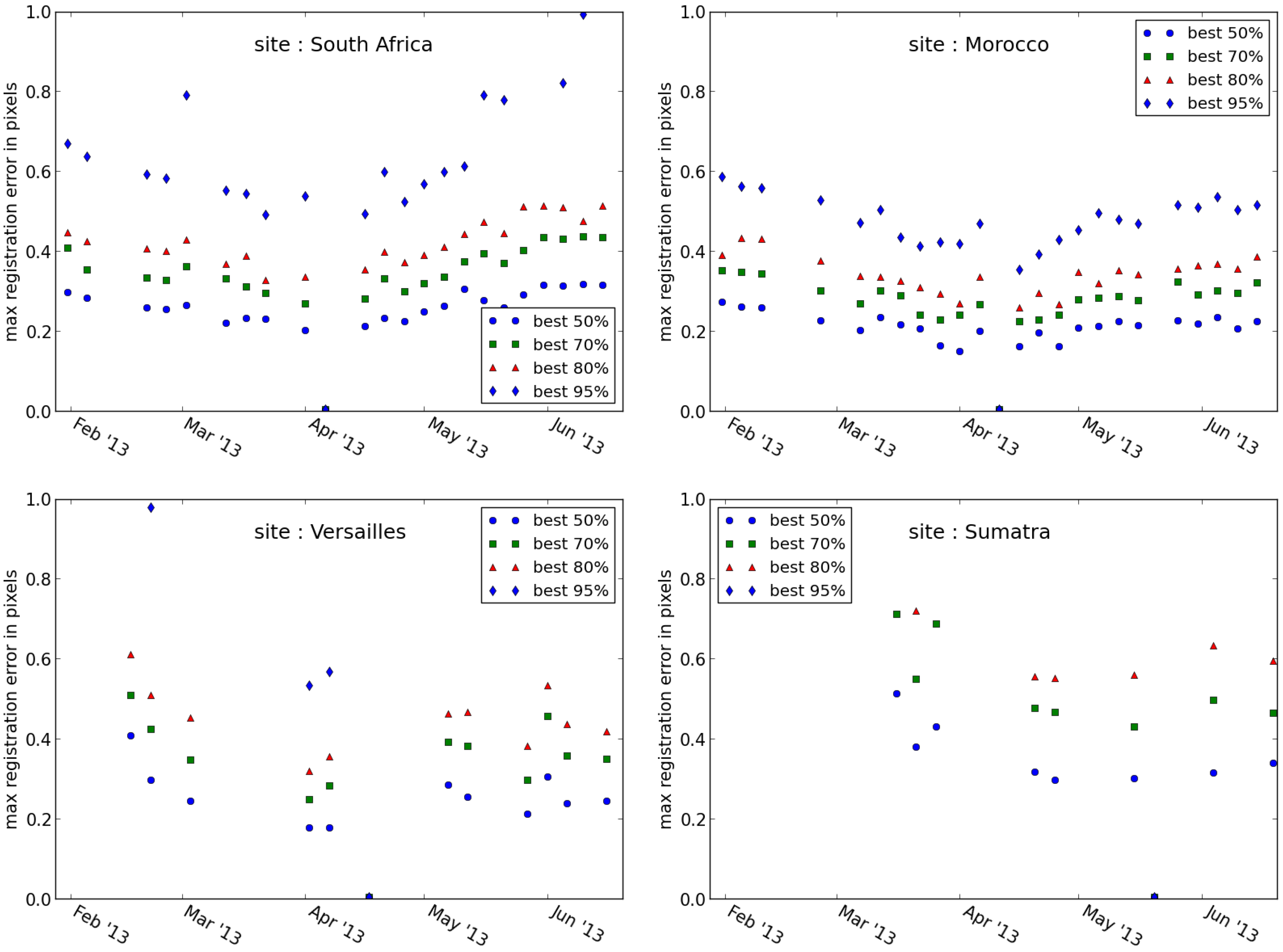
4.2.1. Geometry

As said above, the main difficulty in the Level 1C processor lies in the image ortho-rectification. Reference images were chosen for each site and used to obtain ground control points (GCP), which were used to refine the values of the satellite attitude. As reference images, we used Landsat 8 images acquired in 2013 whenever it was possible. However, for some sites in equatorial regions, no cloud-free Landsat 8 image existed: we had to find images acquired 10 years earlier and even sometimes we had to create a composite image manually from several partially-cloudy images.

The ortho-rectification procedure is somewhat sophisticated [5] and needs to be validated. As the images of SPOT-4 (Take 5) are used as time series, the main performance to check is the multi-temporal registration of images, and unlike many other studies (see for instance [13]), we tried to measure the performances in all conditions of cloudiness and not only on favorable cases with a low cloud cover.

Figure 4 shows the multi-temporal registration error for all of the acquisition dates available on four sites: the first one, South Africa, is a flat site with low cloudiness; the second one, Morocco (1) is a mostly cloud-free site with large variations in elevation, as the Atlas Mountain summit is included in the image; the third one, Versailles, is a flat site with a very large cloud cover in spring 2013; finally, the fourth one, Sumatra, is also a flat site, but nearly always cloudy, with a very uniform forest landscape and large water bodies, whose level and contour change with time: this last site is in fact the worst case encountered in our time series (not accounting for the Borneo site for which no cloud-free reference image was available). The registration performances are computed with regard to a reference image, which is the date with the lowest cloud cover in the SPOT-4 (Take 5) time series. When several images have a similar low cloud cover, the cloud-free date closest to the central date of the time series is selected.

Figure 4. Multi-temporal registration performances obtained for the South Africa, Morocco, Versailles and Sumatra sites, using as a reference the image of the date for which performances are shown equal to zero. The maximum registration error is provided for the best 50%, 70%, 80% and 95% of measurements. In some cases and for the high percentages, the maximum error might exceed one pixel and is not visible in the plot. This happens only for images with a very large cloud cover, but it is always the case for Sumatra.

Figure 4. Multi-temporal registration performances obtained for the South Africa, Morocco, Versailles and Sumatra sites, using as a reference the image of the date for which performances are shown equal to zero. The maximum registration error is provided for the best 50%, 70%, 80% and 95% of measurements. In some cases and for the high percentages, the maximum error might exceed one pixel and is not visible in the plot. This happens only for images with a very large cloud cover, but it is always the case for Sumatra.

The registration accuracy is computed using automatic matching with the MEDICIS software developed by CNES [14,15]. MEDICIS (Moyen d’Evaluation de Décalages entre Images, Commun à l’Imagerie Spatiale) is used for the ortho-rectification of images [5] or for the evaluation of geometric performances [16]. The MEDICIS algorithm is based on the maximum correlation criterion. For a dense grid of points (one point every 20 pixels), the registration error between a master neighborhood of 21 by 21 pixels in the reference image and a slave neighborhood in the assessed image is measured. This method can reach sub-pixel accuracy using correlation, which is done here in the frequency domain. The registration performance is computed only if a minimum of 500 valid correlation matches are found within the grid, out of 22,000 grid points, and a match is declared valid only if the correlation peak is higher than 0.93 and if the master neighborhood standard deviation is high enough.

For each assessed image, the correlation results are ranked in increasing registration error order, and Figure 4 shows the maximum error obtained for each date for the best 50%, 70%, 80% and 95% of pixels. Hereafter, we will refer to the maximum multitemporal registration error for the best X% of pixels as MMRE X. Whereas a visual inspection of the time series does not show a variation of the registration quality for the four sites used in the registration performance measurement, the measured MMRE 95 and even the MMRE 80 over Sumatra or Versailles is often above one pixel and as high as five pixels in some of the Sumatra examples. We have checked visually that these errors do not correspond to actual registration errors, but to measurement errors, due to the presence of often saturated clouds in the evaluated image and for Sumatra in the reference image, as well. It was noted that for images with a large cloud cover, the distribution of errors is far from Gaussian, with MMRE 95 often largely superior to twice MMRE 70, indicating a large presence of outliers.

Hence, the MMRE 70 criterion seems more relevant as a quality index, as it should discard the large correlation errors and as it is very close to the value of the standard deviation for a normal law, which corresponds to the maximum error of the 68% best pixels. Similar studies are usually based on the 90% best pixels instead of 70%, like, for instance, Tao et al. [13], but usually, these performances are measured for cloud-free images, whereas here, images with a very large percentage of clouds are used. We found that the MMRE 70 is nearly always better than 0.4 pixels for Morocco, 0.45 for South Africa, 0.5 pixels for Versailles and 0.7 for Sumatra. For all of these sites, one may notice a clear increase trend of the registration error as a function of the time lag between the reference image and the assessed image. This effect can be explained by the fact that images taken at a few days interval tend to be similar, while images taken with a two-month interval may be very different, therefore reducing the correlation between sliding windows.

This performance produced similar results for most of the tested sites, except one, Congo (2), for which the less cloudy of Landsat 5 images found in the entire Landsat catalog were already very cloudy, and MMRE 70 errors above five pixels have been observed. Among the other sites, a couple of images for which the registration was incorrect was detected through visual control; however, these images had a cloud cover close to 90%, and their MMRE 70 performance could not be measured due to the lack of a sufficient number of GCP.

4.2.2. Radiometry

In this study, we did not control the absolute calibration of SPOT-4 (Take 5), as it is constantly monitored by CNES in the routine phase [17] and as nothing different from the standard processing was done for the experiment.

4.3. L2A Validation

The validation of L2A products focused on three items: the validation of cloud and cloud shadow masks, the validation of the estimation of aerosol optical thickness and, finally, the validation of surface reflectances after atmospheric correction.

4.3.1. Validation of Cloud Masks

For the SPOT-4 (Take 5) experiment, we did not have the manpower to set up an independent dataset to provide a quantitative validation of cloud masks and cloud shadow masks, as done by Zhu et al. in [18]. Our validation of the clouds and cloud shadow masks relied on a visual verification of quick-looks, as shown in Figure 5. In spite of some imperfections, even very thin clouds and their shadows are usually detected.

Although the cloud masks are generally accurate and provide performances similar to those observed when applied to the Landsat 5 and 7 or Formosat-2 satellites in [8], a few defects have been observed, which will require some enhancements in our future works:

• Some cloud classification errors have been observed when the assumption on a slow variation of surface reflectance is wrong, for instance when a wet bare soil dries up and becomes brighter and whiter.
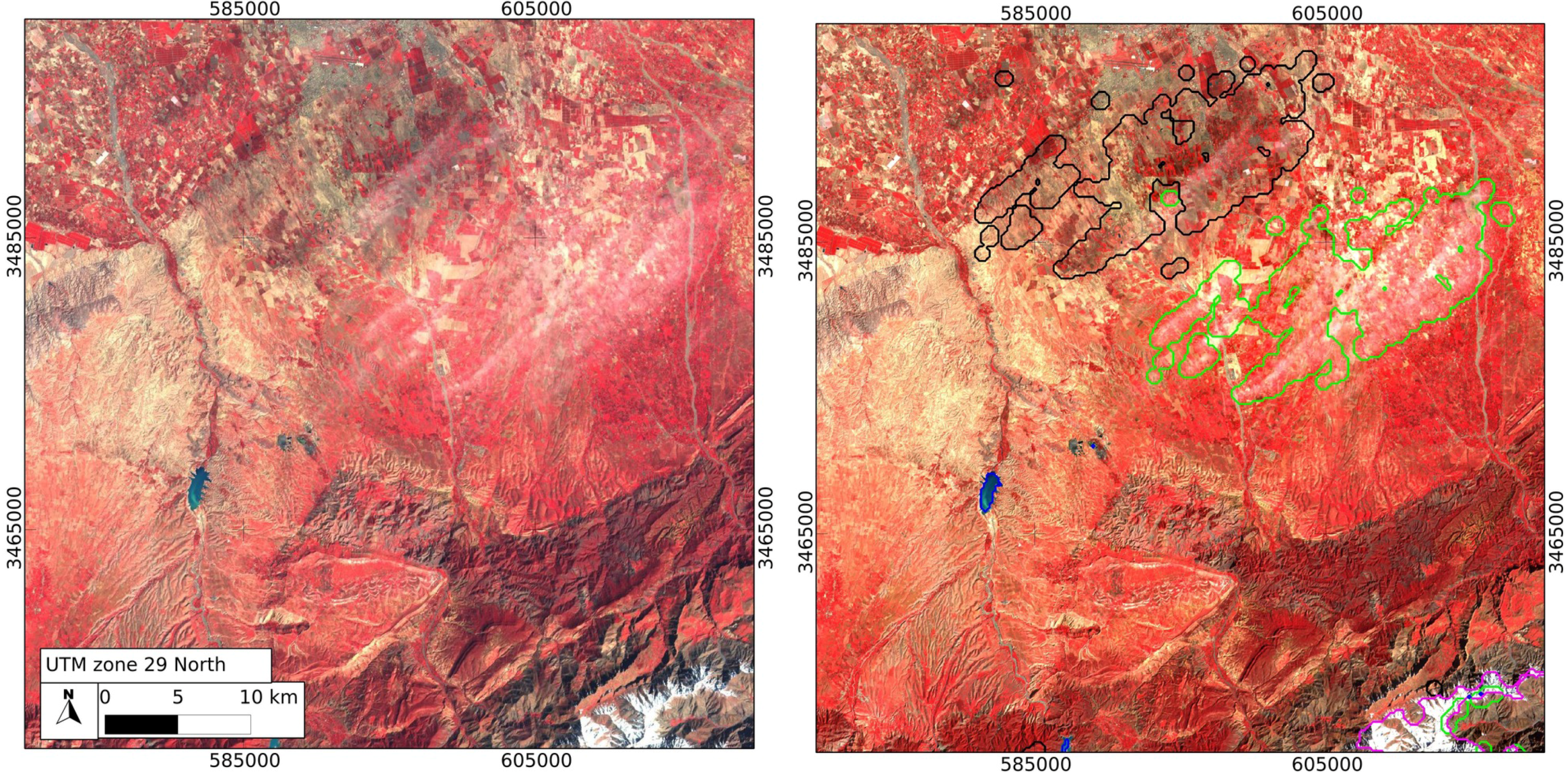
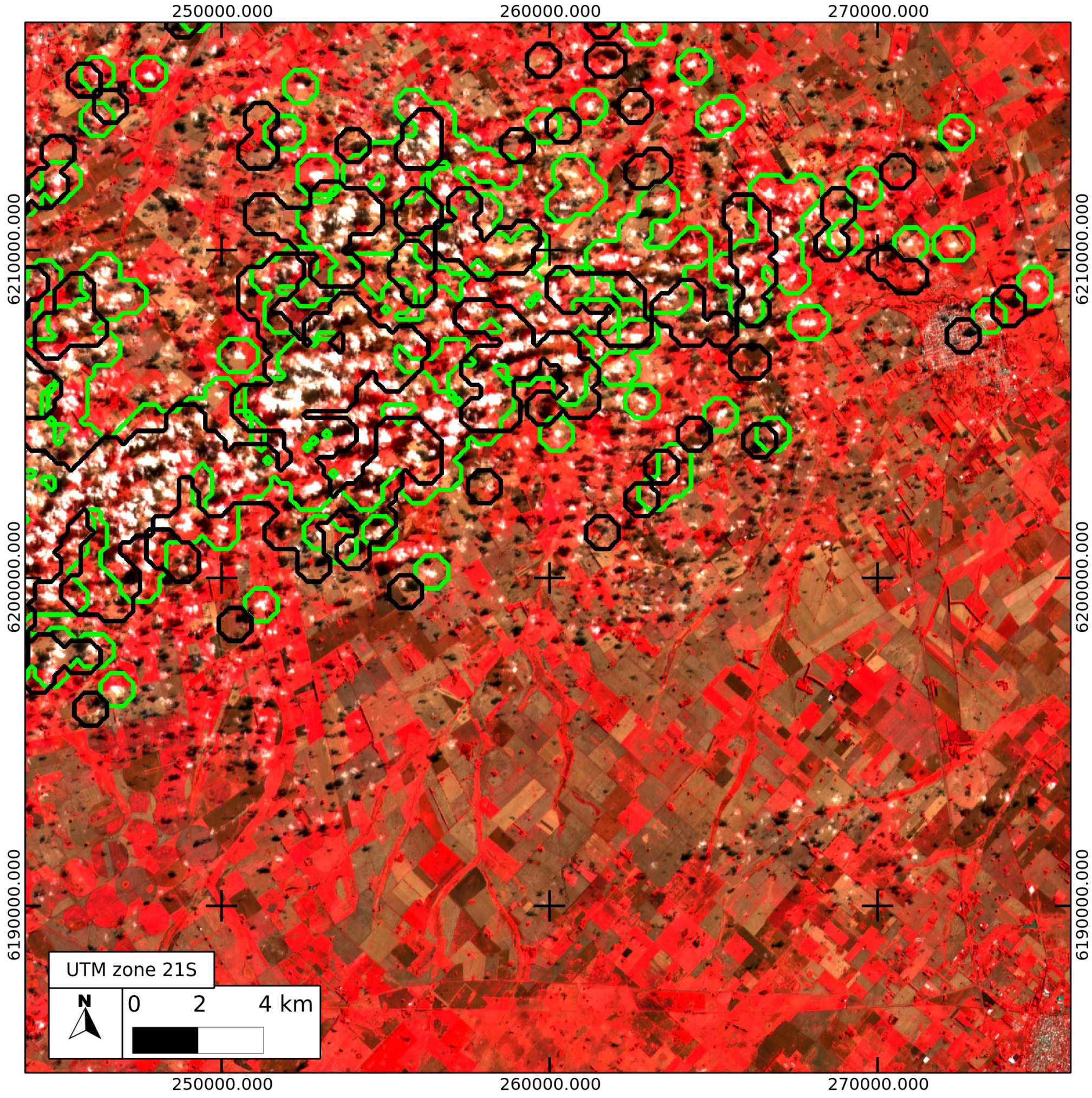
• As the cloud mask was computed at 200-m resolution, some small clouds escape the detection, as shown in Figure 6. To correct this problem, it is straightforward to work at a higher resolution, although, if the resolution is too high, some bright objects, such as buildings, may start to be classified as clouds. As the computer time is also a issue, working at a resolution between 50 and 100 m could be a good compromise. The SPOT-5 (Take 5) cloud mask will be generated at 100-m resolution.
• Over very uniform areas, such as equatorial forests, very thin clouds can easily be detected visually, but some of them may be undetected by our method, since the thresholds are constant throughout the world. As very subtle changes are sought on this kind of landscape, a few users reported that they had to refine the cloud mask. This problem could be solved by tuning the thresholds to stricter values above forests, but in the case of Landsat 8 and Sentinel-2, the band at 1.38 μm will enable one to detect very thin clouds provided they are high enough, reducing this kind of omission.
• Cloud shadows are even more difficult to detect than clouds, because many surfaces can become suddenly darker, such as a bare soil after irrigation or biomass burning. It is therefore difficult to separate the effect of irrigation and the faint shadow of a semi-transparent cloud. It was noticed that all the verifications done to check the validity of the shadow flag, described in the section above, can result in missing some of the real shadow pixels. More work is needed to optimize the cloud shadow mask.

Figure 5. On this SPOT-4 (Take 5) image acquired in Provence, the cloud mask is outlined in green, the cloud shadow mask in black, the water mask in blue and the snow mask in pink (in the northeast corner). One can note that faint clouds and cloud shadows are well detected. Image ©CNES (2013), all rights reserved.

Figure 5. On this SPOT-4 (Take 5) image acquired in Provence, the cloud mask is outlined in green, the cloud shadow mask in black, the water mask in blue and the snow mask in pink (in the northeast corner). One can note that faint clouds and cloud shadows are well detected. Image ©CNES (2013), all rights reserved.

The cloud masks generated on the 45 sites of the SPOT-4 (Take 5) experiment were used to compute valuable statistics on the expected cloud-free repetitivity. The weather in spring 2013 was very cloudy in France, where a large number of sites were located. Some places in the east of France had 30% less sunshine duration than average, and most of the country was at least 10% below. On a few sites (Alsace, Ardeche, Bretagne, Belgium and also China (1) or equatorial sites), only 2–4 cloud-free observations were obtained out of 28 acquisitions from February–mid-June. We also noticed that the number of large images ($110\times 110$ km${}^2$) with no cloud is very low. This fact should push users to develop methods robust to the presence of data gaps due to clouds, otherwise, if only cloud-free images are used, a large proportion of the clear observations at the pixel level will be lost. For instance, on the Belgium site, as shown in Figure 7, only three almost cloud-free images are available, while an average of six cloud-free observations is available at the pixel level.

Figure 6. Example of a SPOT-4 (Take 5) image acquired in Argentina on 29 April with small undetected clouds. The detected clouds are circled in green and their shadows in black.

Figure 6. Example of a SPOT-4 (Take 5) image acquired in Argentina on 29 April with small undetected clouds. The detected clouds are circled in green and their shadows in black.

Figure 7. The left plot shows a map of the number of cloud-free observations (between four and nine), according to the Multi-sensor Atmospheric Correction and Cloud Screening (MACCS) cloud mask, for the site in Belgium, from February–June 2013. The plot on the right shows in blue the percentage of cloud-free pixels for each date. The missing dates are dates with too few cloud-free pixels to allow the ortho-rectification. It should be noted that on that site, the first image of this site with a sufficient number of cloud-free pixels to allow the L1C processing was obtained on 10 March, six weeks after the start of the experiment.

Figure 7. The left plot shows a map of the number of cloud-free observations (between four and nine), according to the Multi-sensor Atmospheric Correction and Cloud Screening (MACCS) cloud mask, for the site in Belgium, from February–June 2013. The plot on the right shows in blue the percentage of cloud-free pixels for each date. The missing dates are dates with too few cloud-free pixels to allow the ortho-rectification. It should be noted that on that site, the first image of this site with a sufficient number of cloud-free pixels to allow the L1C processing was obtained on 10 March, six weeks after the start of the experiment.

Thankfully, a much larger rate of cloud-free data was obtained on several sites, such as Morocco, Provence, Angola and even in Congo (1), where a couple of almost cloud-free images were obtained, which is very unusual.

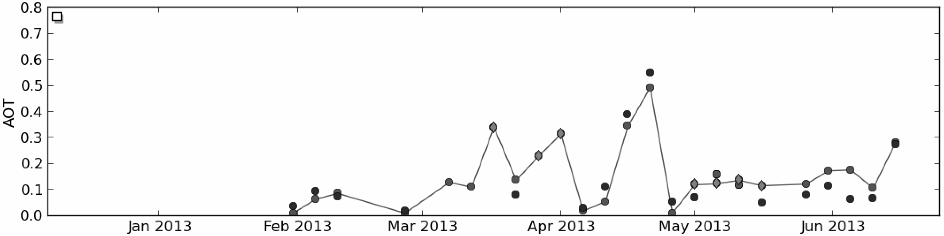
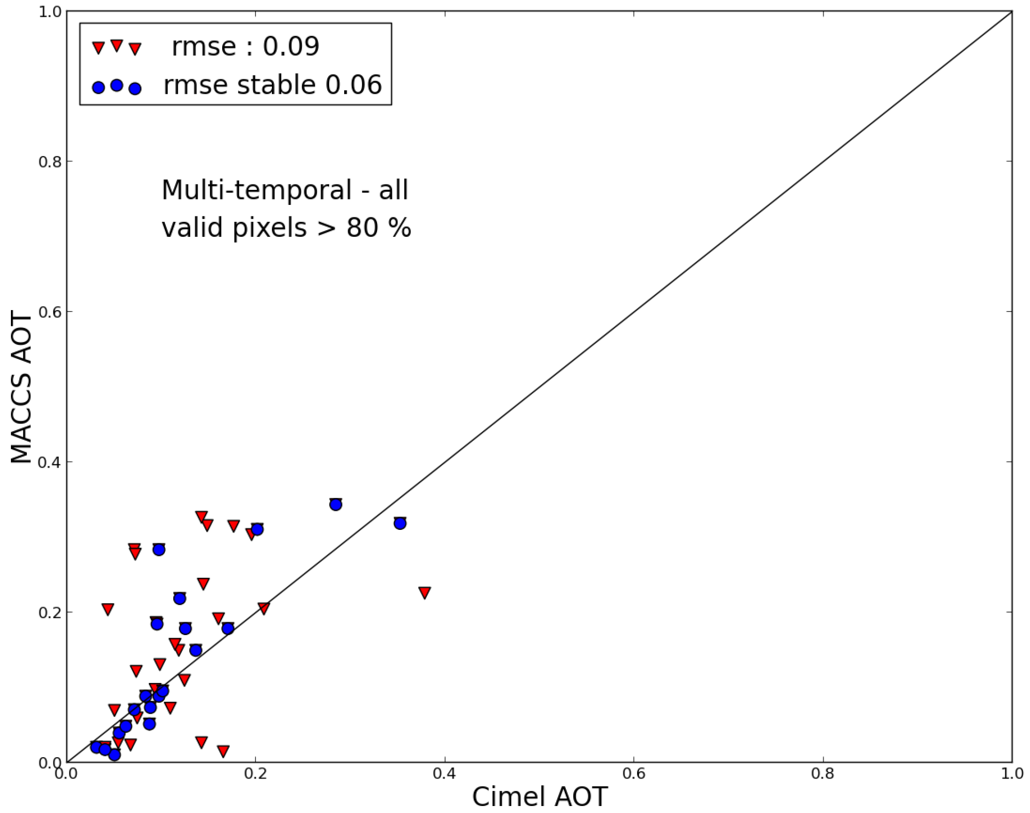
4.3.2. Validation of Aerosol Estimates

One critical point of the accuracy of the surface reflectances contained in the Level 2A products is the AOT estimations. The validation of aerosol optical thickness was performed thanks to the Aerosol Robotic Network (AeroNet), which continuously provides Sun-photometer measurements of the aerosol optical properties above more than 500 sites scattered on all continents [19]. To assess the validity of the estimates obtained by the MACCS multi-temporal method, the AOT retrievals at 0.55 μm were compared to AeroNet in situ data, after an automatic screening of the AeroNet data, which are likely to be corrupted by the presence of clouds. We used Level 1.5 cloud-screened AeroNet data and did some further screening. We used the cloud mask generated on the images to select dates with less than 10% of clouds in a 20-km neighborhood of the AeroNet site, and we only used AeroNet data with an AOT standard deviation below 0.02 within an hour around the satellite overpass time. These criteria define the “stable conditions” in our study, while the other cases are named “unstable conditions”. The image AOT retrievals were averaged on a $20\times 20$ km${}^2$ neighborhood around the AeroNet site. A unique continental aerosol model was used for all of the sites and all of the dates, although better results could probably be obtained with a tuning of the aerosol model for each site.

Figure 8 shows an example of AOT validation for the Morocco site situated near the AeroNet site of Ouarzazate (Morocco). The plot shows that the AOT is measured with a very good accuracy, even on this quasi desert site.

Figure 8. Comparison of MACCS aerosol optical thickness (AOT) estimates at 550 nm (lines) with the AOT measured in situ on the AeroNet site in Ouarzazate (Morocco) (dots), as a function of time.

Figure 8. Comparison of MACCS aerosol optical thickness (AOT) estimates at 550 nm (lines) with the AOT measured in situ on the AeroNet site in Ouarzazate (Morocco) (dots), as a function of time.

The same comparison was done for all of the AeroNet sites that fell within a 50-km distance of a SPOT-4 (Take 5) footprint, considering that the aerosol properties are rather uniform at the scale of a few tens of kilometers. These sites were Arcachon, Carpentras, Seysses, Le Fauga, Palaiseau, Paris and Kyiv in Europe, Saada, Ouarzazate and Ben Salem in Africa, Wallops and Cart Site in America and Gwangjiu in Asia. The validation results are provided in Figure 9.

The standard deviation of AOT estimates in stable cases is 0.06, which is a good result considering the absence of a blue band. However, errors of 0.1 were observed on sites for which the weather was very bad, with less than one clear image per month available and, therefore, an insufficient repetitivity. This is the case for the Ben Salem site in Tunisia, to which the dots with the largest overestimations pertain. In the case of Sentinel-2, the availability of a blue band will enable one to combine a spectral criterion to the multi-temporal one, which should increase the robustness of estimates when long data gaps are observed due to cloud cover. The multi-temporal criterion itself will also lead to enhanced results, because the blue band is less sensitive to vegetation cover variation.

Figure 9. Validation of SPOT-4 (Take 5) AOT estimates with regard to AeroNet in situ measurements over 13 sites in four continents. The blue dots correspond to stable cases, while the red triangles correspond to unstable cases.

Figure 9. Validation of SPOT-4 (Take 5) AOT estimates with regard to AeroNet in situ measurements over 13 sites in four continents. The blue dots correspond to stable cases, while the red triangles correspond to unstable cases.

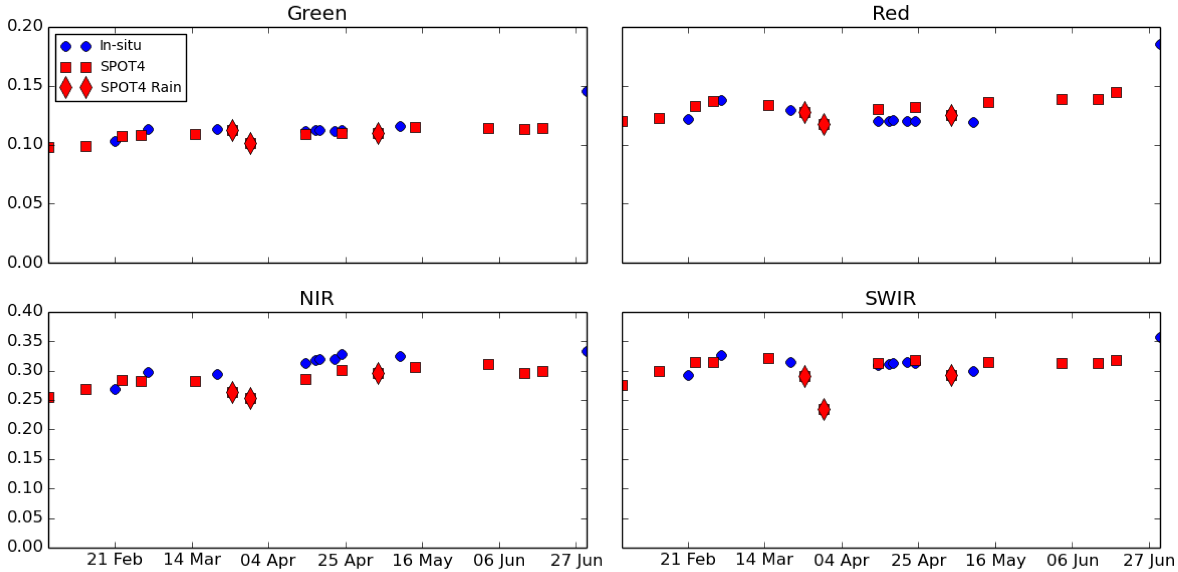
4.3.3. Validation of Surface Reflectances

Thanks to the existence of the AeroNet network of Sun-photometers, the validation of aerosol optical thickness is a convenient, but indirect way to validate the accuracy of surface reflectance, since it addresses the main driver of their accuracy. We decided also to validate the surface reflectances provided in the Level 2A product directly, using two different methods. First, the surface reflectances were compared to in situ measurements obtained at the CNES Robotic Station for Characterizing Atmosphere and Surface (ROSAS) calibration station in La Crau, France, and second, the SPOT-4 (Take 5) surface reflectances were compared to the surface reflectances obtained from NASA’s Moderate-Resolution Imaging Spectroradiometer (MODIS) at a resolution of 0.05 degrees.

Comparison to In Situ Data

The La Crau test site is located in the southeast of France, within the footprint of the SPOT4 (Take 5) Provence site. It is a flat plain of 20 km in diameter covered with white pebbles and grass. It has been used by CNES since 1987 for the absolute radiometric calibration of SPOT cameras and of other satellites. Former calibration activities were conducted during field campaigns devoted to the characterization of the atmosphere and of the site reflectance [20]. In 1997, the ROSAS station was set up on the site on top of a 10 m-high post [21]. Every 90 min, the station measures the solar extinction and the sky radiance to fully characterize the optical properties of the atmosphere at several wavelengths. It also measures the up-welling radiance of the ground to derive the surface reflectance in the direction of observation.

The photometer samples the spectrum from 380 nm to 1600 nm with nine narrow bands. Every non-cloudy day, the photometer automatically and sequentially performs Sun, almucantar (a cone centered on the Sun direction), principal plane (containing the Sun direction and the vertical) and ground measurements. Data are transmitted to CNES and processed there. The projection of the photometer field of view on the ground varies from 20 to 90 cm depending on the viewing angle, and the overall scanned region has a diameter of 17 m. It is compared to the average of Level 2A surface reflectance of the three by three pixel neighborhood around the station. For SPOT-4, it corresponds to a neighborhood of 60 by 60 m.

The photometer calibration (see [21]) is performed in situ using the Sun measurements for irradiance and cross-band calibration and over the Rayleigh scattering for the short wavelength radiance calibration. The data are processed by an operational software, which calibrates the photometer, estimates the atmospheric optical properties and computes the bidirectional reflectance distribution function of the site. This is done by fitting a directional model [22], which allows computing the surface reflectance for any observation geometry. It is therefore possible to use the ROSAS station not only to verify the absolute calibration of sensors, but also to validate the surface reflectance.

Figure 10. Comparison of SPOT-4 (Take 5) surface reflectances with Robotic Station for Characterizing Atmosphere and Surface (ROSAS) reflectances for the four bands of SPOT-4 (Take 5). The blue circles correspond to ROSAS in situ measurements, while the red squares correspond to SPOT-4 (Take 5). Three of them, observed after rain events, are marked by red diamonds.

Figure 10. Comparison of SPOT-4 (Take 5) surface reflectances with Robotic Station for Characterizing Atmosphere and Surface (ROSAS) reflectances for the four bands of SPOT-4 (Take 5). The blue circles correspond to ROSAS in situ measurements, while the red squares correspond to SPOT-4 (Take 5). Three of them, observed after rain events, are marked by red diamonds.

Surface reflectance validation results using ROSAS are shown in Figure 10. The agreement between retrieved and in situ reflectances is better than 5% for the green band (550 nm), the red band (670 nm) and the SWIR (1650 nm), and the reflectances observed are as smooth as those observed in situ. A bias (7%–8%) is observed for the NIR band (840 nm), that may be partly explained by the lack of a radiometer spectral band near the center wavelength of this band. Indeed, for each SPOT-4 spectral band, the comparison is obtained thanks to a spectral interpolation of the reflectances measured by the station in the two nearest bands of the ROSAS radiometer, but in the NIR, the spectral bands available in ROSAS are quite far from the ones of SPOT-4. Moreover, the spectral interpolation could be biased because the SPOT-4 B3 band is a wide band overlapping the red-edge region. An improvement of the spectral interpolation method, where the true spectral reflectance is fitted to the data, is under qualification and should lead to a decrease of systematic uncertainties in this specific spectral region. The photometer field of view is also known only with an accuracy of 5% for the visible and NIR bands, and SPOT-4 absolute calibration is provided with an accuracy estimated to 5%.

The surface reflectances estimated in the SWIR band by SPOT-4 (Take 5) appear noisier than for the other bands, but the lowest reflectances measured by SPOT-4 (Take 5) in the SWIR turn out to be due to a higher soil moisture, caused by rain events that occurred just before the acquisitions marked by diamonds in Figure 10. The corresponding measurements were not available for the ROSAS station, because a nearly complete cloud-free day of observation is necessary to produce an estimation of the surface reflectance.

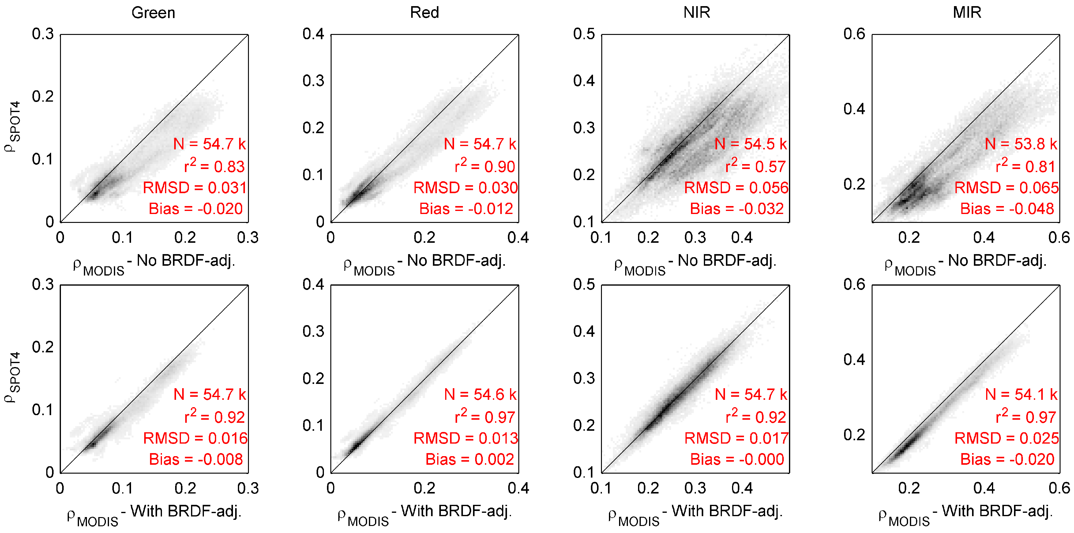
Cross-Comparison with MODIS Surface Reflectances

An additional evaluation experiment was led at NASA and University of Maryland. It is based on the cross-comparison of SPOT-4 (Take-5) surface reflectances with the MODIS surface reflectances, considered as the reference dataset and derived from the MOD09CMG product (MODIS product nÂř9 sampled at 0.05 degrees). The cross-comparison is structured in two processing steps: (i) averaging the SPOT-4 SR data to 0.05 degrees; and (ii) bidirectional reflectance distribution function (BRDF) adjustments of the MODIS surface reflectance to the corresponding SPOT-4 Sun and view geometry. As MODIS and SPOT4 spectral response are not identical, an adjustment of the spectral responses would have been justified, but was not done in this study.

The BRDF adjustment methodology is the same as the one used by [23] to cross-compare Landsat and MODIS data and relying on the BRDF approach introduced by [24]. The study is based on the comparison of aggregated 0.05 degree pixels (about 5 km) considering only cloud-free, cloud shadow-free, snow-free and water-free SPOT-4 pixels from all SPOT-4 (Take-5) sites, with similar pixels acquired on the same day by the MODIS sensor onboard the Terra satellite. This comparison represents more than 50 thousand 0.05 degree pixels.

The results of the cross-comparison of SPOT-4 and MODIS SR data are displayed in Figure 11. We showed the cross-comparison before and after BRDF adjustment to outline the necessity to perform this adjustment, as well as the good performances of the approach [24] used to adjust the MODIS BRDF. With BRDF adjustment, the agreement becomes excellent, with low biases and an RMS error below 0.017 for all bands, except in the SWIR (0.025), where the interpolation of dead detectors in the SPOT-4 (Take 5) might contribute largely.

The very good agreements for the red and the NIR bands confirm altogether the inter-consistency of the SPOT-4 (Take-5) and MODIS data absolute calibration, as well as the quality of atmospheric correction, cloud screening and BRDF adjustment. Taking into account residual errors in BRDF adjustment and an equivalent atmospheric correction error for both sensors, this means that the RMS atmospheric correction error at 5-km resolution for both sensors has an order of magnitude close to 0.01. The higher level of bias for the green and SWIR band is probably due to the spectral differences between both sensors, which are larger in these bands, but the very low bias for the two other bands might also be degraded by a spectral adjustment, which was not performed in this study.

Figure 11. Comparison of SPOT-4 (Take 5) surface reflectances with MODIS reflectances averaged at 5-km resolution, for all SPOT-4 (Take 5) acquisition dates; top, before directional correction; bottom, after directional correction. From left to right, the columns correspond to the green, red, NIR and SWIR bands.

Figure 11. Comparison of SPOT-4 (Take 5) surface reflectances with MODIS reflectances averaged at 5-km resolution, for all SPOT-4 (Take 5) acquisition dates; top, before directional correction; bottom, after directional correction. From left to right, the columns correspond to the green, red, NIR and SWIR bands.

5. Conclusion and Lessons Learned

The main objective of the SPOT-4 (Take 5) experiment was to help future Sentinel-2 users get a glimpse of the interest and opportunities brought by the new mission, so that they start to get ready to use them, develop new processing methods and test new applications. For this purpose, 45 sites with very diverse types of landscapes were chosen, and the data were freely and openly distributed to the international scientific community. As more than 600 different users from at least 28 countries downloaded the data, it may be qualified as a success. The most frequently-received feedback concerns the usefulness of Level 2A products (76% of the downloads correspond to Level 2A products and only 24 to Level 1C), and on some cloudy sites, it was reported that the five-day repetitivity might be insufficient.

On the scientific side, five months of data are often not enough to allow one to obtain publishable results, but nonetheless, several articles have been published so far. A subset of the applications of the experiment is shown on this Special Issue in MDPI remote sensing: “Lessons Learned from the SPOT-4 (Take 5): Experiment in Preparation for Sentinel-2”. Before this Special Issue, a few articles using time series of SPOT-4 (Take 5) images were already published regarding the estimation of water needs ([25] and [26]) or forestry [27].

To allow the distribution of data, a new ground segment was set up at the Theia land data center to produce and distribute Level 1C and Level 2A data. The processing of Level 1C with a sub-pixel multi-temporal registration accuracy in a fully automatic way was quite a challenge, as the initial location error of SPOT-4 has a standard deviation above 20 pixels, and peak values of 75 pixels were observed; moreover, our will to process all of the images for which a few km${}^2$ of cloud-free land were available did not ease the task. However, this processing was successful in most of the cases, except for a uniform equatorial forest site always covered by clouds in Congo.

The lack of a blue band could also have degraded the performances of the cloud detection and of the aerosol estimates for the Level 2A product, as the classical methods for cloud detection and atmospheric correction usually rely on that band. Thankfully, the observations with constant viewing angles allowed us to use multi-temporal methods to detect the clouds and to estimate the AOT, and even if a blue band is better suited, even for the multi-temporal method, replacing it by the green band was successful. The MACCS Level 2A processor provided very good results, without needing tuning work to adapt it from Landsat or Formosat-2 data, which had been used to test it. The masks are very accurate, and the atmospheric correction is quite good, when the number of cloud-free images is sufficient and when the selected aerosol model is correct. However, additional work is still needed to find a method to select the aerosol model for each region, either from climatologies or from new weather analyses that provide aerosol optical thickness estimates for several types of models (Monitoring Atmospheric Composition and Climate model (MACC) [28] or the Goddard Earth Observing System Model, Version 5 (GEOS-5) [29] model).

Sentinel-2 will offer more spectral bands to improve the results, and the presence of two blue bands (440 and 490 nm) will enable one to combine multi-temporal and multi-spectral criteria over vegetated zones to allow a significant improvement in terms of quality. From 2016 on, the MACCS processor will be applied to Sentinel-2 data at the Theia Land Data Center at the European scale to produce Level 2A products.

The SPOT-4 (Take 5) dataset is still open to the scientific community and also to private companies, with a very open license. The data may be downloaded from https://spot-take5.org. Thanks to the success of the SPOT-4 (Take 5) experiment, CNES and ESA accepted renewing the Take 5 experiment with the SPOT-5 satellite, from April–August 2015. This new experiment is based on 150 sites and provides images with the same spatial resolution as Sentinel-2. Although data are acquired in all continents and all sorts of biomes, the time period is perfectly suited to monitor vegetation cover and, particularly, summer crops in the Northern Hemisphere. As for SPOT-4 (Take 5), L1C and L2A products will be freely available for users. The data may be downloaded from the same site as SPOT-4 (Take 5) data.

References

- Drusch, M.; Del Bello, U.; Carlier, S.; Colin, O.; Fernandez, V.; Gascon, F.; Hoersch, B.; Isola, C.; Laberinti, P.; Martimort, P.; et al. Sentinel-2: ESA’s Optical High-Resolution Mission for GMES Operational Services. Remote Sens. Environ. 2012, 120, 25–36. [Google Scholar] [CrossRef]
- Maisongrande, P.; Duchemin, B.; Dedieu, G. VEGETATION/SPOT: An operational mission for the Earth monitoring; presentation of new standard products. Int. J. Remote Sens. 2004, 25, 9–14. [Google Scholar] [CrossRef]
- Tinel, C.; Fontannaz, D.; de Boissezon, H.; Grizonnet, M.; Michel, J. The ORFEO acompaniment program and ORFEO ToolBox. IGARSS 2012. [Google Scholar] [CrossRef]
- Hagolle, O.; Huc, M.; Villa Pascual, D.; Dedieu, G. A multi-temporal and multi-spectral method to estimate aerosol optical thickness over land, for the atmospheric correction of FormoSat-2, LandSat, VENµS and Sentinel-2 images. Remote Sens. 2015, 7, 2668–2691. [Google Scholar] [CrossRef]
- Bignalet-Cazalet, F.; Baillarin, S.; Greslou, D.; Panem, C. Automatic and generic mosaicing of satellite images. IGARSS 2010. [Google Scholar] [CrossRef]
- Baillarin, S.; Gigord, P.; Hagolle, O. Automatic registration of optical images, a stake for future missions: Application to ortho-rectification, time series and mosaic products. IGARSS 2008. [Google Scholar] [CrossRef]
- Hagolle, O.; Dedieu, G.; Mougenot, B.; Debaecker, V.; Duchemin, B.; Meygret, A. Correction of aerosol effects on multi-temporal images acquired with constant viewing angles: Application to Formosat-2 images. Remote Sens. Environ. 2008, 112, 1689–1701. [Google Scholar] [CrossRef] [Green Version]
- Hagolle, O.; Huc, M.; Villa Pascual, D.; Dedieu, G. A multi-temporal method for cloud detection, applied to Formosat-2, VENμS, Landsat and Sentinel-2 images. Remote Sens. Environ. 2010, 114, 1747–1755. [Google Scholar] [CrossRef] [Green Version]
- Arnaud, M.; Leroy, M. SPOT 4: A new generation of SPOT satellites. ISPRS J. Photogramm. Remote Sens. 1991, 46, 205–215. [Google Scholar] [CrossRef]
- Kubik, P.; Breton, E.; Meygret, A.; Cabrieres, B.; Hazane, P.; Leger, D. SPOT4 HRVIR first in-flight image quality results. Proc. SPIE 1998. [Google Scholar] [CrossRef]
- Meygret, A.; Dinguirard, M.C.; Henry, P.J.; Poutier, L.; Lafont, S.; Hazane, P. SPOT Histogram data base. Proc. SPIE 1997. [Google Scholar] [CrossRef]
- Moy, J.P.; Hugon, X.; Chabbal, J.; De Cachard, J.; Lenoble, C.; Mollaret, D.; Villard, M.; Villotitch, B. 3000 In Ga As Photodiode Multiplexed Linear Array For The Spot 4 S.W.I.R. Channel. Proc. SPIE 1989. [Google Scholar] [CrossRef]
- Tao, C.V.; Hu, Y.; Jiang, W. Photogrammetric exploitation of IKONOS imagery for mapping applications. Int. J. Remote Sens. 2004, 25, 2833–2853. [Google Scholar] [CrossRef]
- Berthier, E.; Vadon, H.; Baratoux, D.; Arnaud, Y.; Vincent, C.; Feigl, K.L.; Rémy, F.; Legrésy, B. Surface motion of mountain glaciers derived from satellite optical imagery. Remote Sens. Environ. 2005, 95, 14–28. [Google Scholar] [CrossRef]
- Rosu, A.M.; Pierrot-Deseilligny, M.; Delorme, A.; Binet, R.; Klinger, Y. Measurement of ground displacement from optical satellite image correlation using the free open-source software MicMac. ISPRS J. Photogramm. Remote Sens. 2015, 100, 48–59. [Google Scholar] [CrossRef]
- Bicheron, P.; Amberg, V.; Bourg, L.; Petit, D.; Huc, M.; Miras, B.; Brockmann, C.; Hagolle, O.; Delwart, S.; Ranera, F.; Leroy, M.; Arino, O. Geolocation Assessment of MERIS GlobCover Orthorectified Products. IEEE Trans. Geosci. Remote Sens. 2011, 49, 2972–2982. [Google Scholar] [CrossRef] [Green Version]
- Meygret, A. Absolute calibration: From SPOT1 to SPOT5. Proc. SPIE 2005. [Google Scholar] [CrossRef]
- Zhu, Z.; Woodcock, C.E. Object-based cloud and cloud shadow detection in Landsat imagery. Remote Sens. Environ. 2012, 118, 83–94. [Google Scholar] [CrossRef]
- Holben, B.N.; Eck, T.F.; Slutsker, I.; Tanré, D.; Buis, J.P.; Setzer, A.; Vermote, E.; Reagan, J.A.; Kaufman, Y.J.; Nakajima, T.; et al. AERONET—A federated instrument network and data archive for aerosol characterization. Remote Sens. Environ. 1998, 66, 1–16. [Google Scholar] [CrossRef]
- Santer, R.; Gu, X.F.; Guyot, G.; Deuzé, J.L.; Devaux, C.; Vermote, E.; Verbrugghe, M. SPOT calibration at the La Crau test site (France). Remote Sens. Environ. 1992, 41, 227–237. [Google Scholar] [CrossRef]
- Meygret, A.; Santer, R.P.; Berthelot, B. ROSAS: A robotic station for atmosphere and surface characterization dedicated to on-orbit calibration. Proc. SPIE 2011. [Google Scholar] [CrossRef]
- Roujean, J.L.; Leroy, M.; Deschamps, P.Y. A bidirectional reflectance model of the Earth’s surface for the correction of remote sensing data. J. Geophys. Res.: Atmos. 1992, 97, 20455–20468. [Google Scholar] [CrossRef]
- Claverie, M.; Vermote, E.F.; Franch, B.; Masek, J.G. Evaluation of the Landsat-5 TM and Landsat-7 ETM+ surface reflectance products. Remote Sens. Environ. 2014, in press. [Google Scholar]
- Vermote, E.; Justice, C.O.; Breon, F.M. Towards a generalized approach for correction of the BRDF effect in MODIS directional reflectances. IEEE Trans. Geosci. Remote Sens. 2009, 47, 898–908. [Google Scholar] [CrossRef]
- Le Page, M.; Toumi, J.; Khabba, S.; Hagolle, O.; Tavernier, A.; Kharrou, M.H.; Er-Raki, S.; Huc, M.; Kasbani, M.; Moutamanni, A.E.; et al. A life-size and near real-time test of irrigation scheduling with a Sentinel-2 Like Time Series (SPOT4-Take5) in Morocco. Remote Sens. 2014, 6, 11182–11203. [Google Scholar] [CrossRef]
- Akdim, N.; Alfieri, S.M.; Habib, A.; Choukri, A.; Cheruiyot, E.; Labbassi, K.; Menenti, M. Monitoring of irrigation schemes by remote sensing: Phenology versus retrieval of biophysical variables. Remote Sens. 2014, 6, 5815–5851. [Google Scholar] [CrossRef]
- Miettinen, J.; Stibig, H.J.; Achard, F.; Hagolle, O.; Huc, M. First assessment on the potential of Sentinel-2 data for land area monitoring in Southeast Asian conditions. Asian J. Geoinf. 2015, 15, 23–30. [Google Scholar]
- Benedetti, A.; Morcrette, J.J.; Boucher, O.; Dethof, A.; Engelen, R.J.; Fisher, M.; Flentje, H.; Huneeus, N.; Jones, L.; Kaiser, J.W. Aerosol analysis and forecast in the European Centre for Medium-Range Weather Forecasts Integrated Forecast System: 2. Data assimilation. J. Geophys. Res. 2009, 114, D13205. [Google Scholar] [CrossRef]
- Suarez, M.J.; Rienecker, M.M.; Todling, R.; Bacmeister, J.; Takacs, L.; Liu, H.C.; Gu, W.; Sienkiewicz, M.; Koster, R.D.; Gelaro, R.; et al. The GEOS-5 Data Assimilation System. Documentation of Versions 5.0. 1, 5.1. 0, and 5.2. 0. 2008. [Google Scholar]
© 2015 by the authors; licensee MDPI, Basel, Switzerland. This article is an open access article distributed under the terms and conditions of the Creative Commons Attribution license (http://creativecommons.org/licenses/by/4.0/).
Share and Cite
Hagolle, O.; Sylvander, S.; Huc, M.; Claverie, M.; Clesse, D.; Dechoz, C.; Lonjou, V.; Poulain, V. SPOT-4 (Take 5): Simulation of Sentinel-2 Time Series on 45 Large Sites. Remote Sens. 2015, 7, 12242-12264. https://doi.org/10.3390/rs70912242
Hagolle O, Sylvander S, Huc M, Claverie M, Clesse D, Dechoz C, Lonjou V, Poulain V. SPOT-4 (Take 5): Simulation of Sentinel-2 Time Series on 45 Large Sites. Remote Sensing. 2015; 7(9):12242-12264. https://doi.org/10.3390/rs70912242
Chicago/Turabian StyleHagolle, Olivier, Sylvia Sylvander, Mireille Huc, Martin Claverie, Dominique Clesse, Cécile Dechoz, Vincent Lonjou, and Vincent Poulain. 2015. "SPOT-4 (Take 5): Simulation of Sentinel-2 Time Series on 45 Large Sites" Remote Sensing 7, no. 9: 12242-12264. https://doi.org/10.3390/rs70912242