Assessment of an Operational System for Crop Type Map Production Using High Temporal and Spatial Resolution Satellite Optical Imagery

Abstract

Crop area extent estimates and crop type maps provide crucial information for agricultural monitoring and management. Remote sensing imagery in general and, more specifically, high temporal and high spatial resolution data as the ones which will be available with upcoming systems, such as Sentinel-2, constitute a major asset for this kind of application. The goal of this paper is to assess to what extent state-of-the-art supervised classification methods can be applied to high resolution multi-temporal optical imagery to produce accurate crop type maps at the global scale. Five concurrent strategies for automatic crop type map production have been selected and benchmarked using SPOT4 (Take5) and Landsat 8 data over 12 test sites spread all over the globe (four in Europe, four in Africa, two in America and two in Asia). This variety of tests sites allows one to draw conclusions applicable to a wide variety of landscapes and crop systems. The results show that a random forest classifier operating on linearly temporally gap-filled images can achieve overall accuracies above 80% for most sites. Only two sites showed low performances: Madagascar due to the presence of fields smaller than the pixel size and Burkina Faso due to a mix of trees and crops in the fields. The approach is based on supervised machine learning techniques, which need in situ data collection for the training step, but the map production is fully automatic.

1. Introduction

1.1. The Need for Crop Type Maps

The increasing needs in food supply in the near future will require higher agricultural yields [1]. Other factors increasing the pressure on agricultural lands are urban expansion and the production of bio-fuels [2,3,4]. These pressures will also have consequences on natural ecosystems [5,6]. Indeed, agricultural activities are a major cause of ecosystem degradation at the global scale [7], and therefore, land use change monitoring related to farming is crucial for sustainable land management [8].

Crop area extent estimates and crop type maps provide crucial information for agricultural monitoring and management. Remote sensing imagery in general and, in particular, high temporal and high spatial resolution data as the ones which will be available with upcoming systems, such as Sentinel-2 [9], constitute a major asset for this kind of application.

1.2. Sentinel-2 for Agriculture

The Sentinel-2 for Agriculture project funded by the European Space Agency [10] aims at fully exploiting the unprecedented Sentinel-2 observational capabilities for agricultural monitoring through the development of open source processing chains capable of large-scale production. Responding to the GEO Global Agricultural Monitoring (GEOGLAM) target product [11], three Earth Observation products—dynamic cropland mask, crop type and crop status—have been identified for these processing chains and will be demonstrated at the national scale.

One of these products is crop type maps with spatial resolutions between 10 to 20 m and very high constraints in terms of thematic accuracy.

The following specifications of the crop type map product are based on the requirements from an international user group of agricultural institutions and stakeholders collected during the project. The nomenclature (the list of mapped crop type classes) of the maps is tailored for each country and includes the main regional crop types or crop groups, including the distinction between rain-fed and irrigated crops. This product should be delivered as soon as possible after the end of the season, with an early delivery after the first half of the season. The latter will be of lesser quality, yet useful for some applications. In this paper, we focus on the former, the product at the end of the season.

In the frame of this project and in cooperation with the JECAM [12] initiative, 12 test sites scattered around the globe covering large areas have been used for method development, prototyping and validation. For this, simulations of Sentinel-2 time series based on SPOT4 (Take5) [13] and Landsat 8 data [14] were used.

In the last phase of the project, three complete countries (about 500,000 km${}^2$) and five local sites of 290 km × 290 km will be processed using real Sentinel-2 data. Therefore, these processing chains will have to deal with huge amounts of data, different kinds of agricultural systems and different eco-climatic areas. These constraints imply the use of techniques minimizing human operation and having sufficient flexibility in order to cope with very different operational conditions.

1.3. Previous Works

To the best of our knowledge, no annual crop type product has ever been generated operationally at a country scale at 10-m resolution (or even 30 m). Indeed, there is no literature or publicly-available product corresponding to these characteristics, although similar initiatives exist.

For instance, global irrigation maps [15] have been produced using a mix of remote sensing imagery, climate data and national surveys. Recently, a 1-km global cropland percentage map for the baseline year 2005 has been released [16]. It uses an approach that integrates a number of individual cropland maps at global, regional or national scales (GlobCover 2005 [17] and MODIS, v.5 [18]), regional land cover maps (AFRICOVER) and national maps from mapping agencies and other organizations. However, these products do not fulfil the GEOGLAM target products and user requirements collected during the Sentinel-2 Agriculture project in terms of spatial resolution and timeliness.

As pointed out by [19], continental- or even global-scale analysis using remote sensing imagery, such as Landsat’s, was generally regarded as not feasible because of the absence of well-registered multi-temporal datasets, skills and processing power. This has now been overcome, but even with the availability of the Landsat WELDdata, the insufficient temporal revisit of 16 days and the spatial resolution of 30 m, the generation of accurate crop type products remains difficult.

The requirements for general land cover products were well identified by Whitcraft et al. in [20,21], but the crop type product needs in many cases a finer spatial resolution than Landsat’s. Furthermore, for many locations on Earth, a higher temporal revisit is needed in order to maximize the chances of getting cloud-free data: the growing cycle of vegetation in agriculture needs finer temporal resolutions than those needed for some existing forest studies [22]. For instance, summer crops, such as sunflower and maize, may be separated thanks to the longer growing period of the maize.

One of the first works using multi-temporal (only three dates) Landsat imagery for crop mapping is [23], where the proportion of corn and soybean was estimated. Although Landsat’s resolution could have allowed it, no field-level mapping was performed, and only two classes were taken into account.

Twenty years later [24], a higher number of dates were being used, and field level mapping was performed, but still limited to one or two classes. Brown et al. [25] acknowledge that much additional research is required to fully and reliably differentiate more specific crop classes.

On the other hand, while high resolution data have not been exploited for operational crop type mapping, many efforts have been devoted to the use of MODIS imagery for this purpose. For instance, Wardlow et al. [26] used MODIS for annual crop maps. For this mid-resolution imagery, unmixing approaches have been proposed in order to estimate sub-pixel proportions [27,28], but the field level remains inaccessible. Similar works have been proposed using SPOT-Vegetation [29].

Since the availability of the WELD data, interesting attempts at general land cover mapping using Landsat at the continental scale have been carried out. For instance, Hansen et al. [30] performed 30-m annual land cover estimates of trees, other vegetation (including grasses, shrubs and forbs), bare ground cover and water presence over the continental USA.

As stated above, crop type mapping at large scales and with high resolution imagery is non existent in the literature. Even recent literature uses limited nomenclatures [31]. This is not to say that there are no crop monitoring systems. The reader can refer to [32] where the last generation of the Chinese global CropWatch system is described. The same reference cites other similar existing systems. However, these systems provide statistics at the global, national or regional level, but are not able to provide crop mapping at the field level.

1.4. Goals of This Work

The goal of the work presented in this paper is to assess to what extent state-of-the-art supervised classification methods can be applied to high resolution multi-temporal optical imagery to produce accurate crop type maps at the global scale, that is for different landscapes, climatic areas and crop systems.

Five concurrent strategies for automatic crop type map production have been selected and benchmarked in order to cover a wide spectrum of approaches. The selection of five strategies cannot be based only on a literature review, since by definition, there are no existing works using Sentinel-2-like data. Only recently, thanks to the SPOT4 (Take5) experiment [33], data with specifications similar to Sentinel-2 in terms of spatial and temporal resolution have been made available. This paper presents a summary of the results of the benchmarking of the selected five strategies on SPOT4 (Take5) data over 12 test sites. The results obtained in this work show the potential of the Sentinel-2 system in the sense that the same processing chain can be applied to Sentinel-2 imagery. Sentinel-2 will bring a better spectral sensitivity and a higher spatial resolution, allowing one to achieve even better results.

The paper is organized as follows. In Section 2, we present the data sources used in this work (Section 2.1) and the design of the processing chains and the associated experiments (Section 2.2). Section 3 presents the results and a detailed discussion. Finally, Section 4 draws the conclusion.

2. Materials and Methods

2.1. Data Sources

In order to produce a reliable assessment of the crop type mapping system, 12 sites spread all over the world were used. The list includes 4 sites in African countries where the stakes of food security are highest: Morocco, Madagascar, Burkina Faso and South Africa. To give an answer to the global agricultural variability, also sites in Asia (China, Pakistan), Europe (France, Belgium, Ukraine, Russia), North America (USA) and South America (Argentina) were included. A large variety of climate types and agricultural practices are therefore represented. For all of these sites, satellite imagery (Section 2.1.1) and in situ data (Section 2.1.2) were available.

2.1.1. Satellite Imagery

The SPOT4 (Take5) and Landsat 8 data were processed to Level 2A (i.e., surface reflectance values with masks for clouds, cloud shadows, snow and water), as described in [13], using the Multi-Sensor Atmospheric Correction and Cloud Screening (MACCS) processor, developed and maintained at the Centre d’Etudes Spatiales de la BIOsphère (CESBIO; [34]).

For SPOT4, the 4 spectral bands (green, red, NIR and SWIR) at 20-m resolution were used. For Landsat 8, only 6 out of the 8 spectral bands at 30-m resolution were used (blue, green, red, NIR, SWIR1, SWIR2), since the coastal and the aerosol bands are not pertinent for vegetation mapping. For 2 of the sites (Pakistan and Russia), RapidEye imagery was also used because of the low number of available SPOT4 and Landsat 8 acquisitions. In this case, the blue, green, red, red-edge and NIR bands were used. Although these images were provided with 5-m resolution, they were resampled to 20 m using the SPOT4 sampling grid as a reference.

The quantity and the quality of these data were not homogeneous across sites, depending mainly on the observed cloud cover. We briefly describe each dataset below. Geographical coordinates of the center of each site, as well as their sizes are given.

• Argentina (59.617343W, 34.227771S, 3481 km${}^2$), very good: Very good coverage (almost one acceptable image per week) from February to April covering the end of the summer crop season (October/November to April). Winter crops are not covered at all.
• Belgium (4.953034E, 50.635297N, 3829 km${}^2$), moderate: Due to high cloudiness, the image dataset is not very rich, but has at least one acceptable image per month during the summer crop season (from March to September), covering also the end of the winter crop season.
• Burkina Faso (3.669765W, 11.257590N, 6734 km${}^2$), bad: Very few images in the growing period.
• China (116.503414E, 36.817027N, 3847 km${}^2$), moderate: The dataset has a high presence of aerosols in February and March. April and May are well covered, as well as the beginning of June. The end of winter crops will be well covered, and it was possible to work (not in the best conditions) with the summer crops.
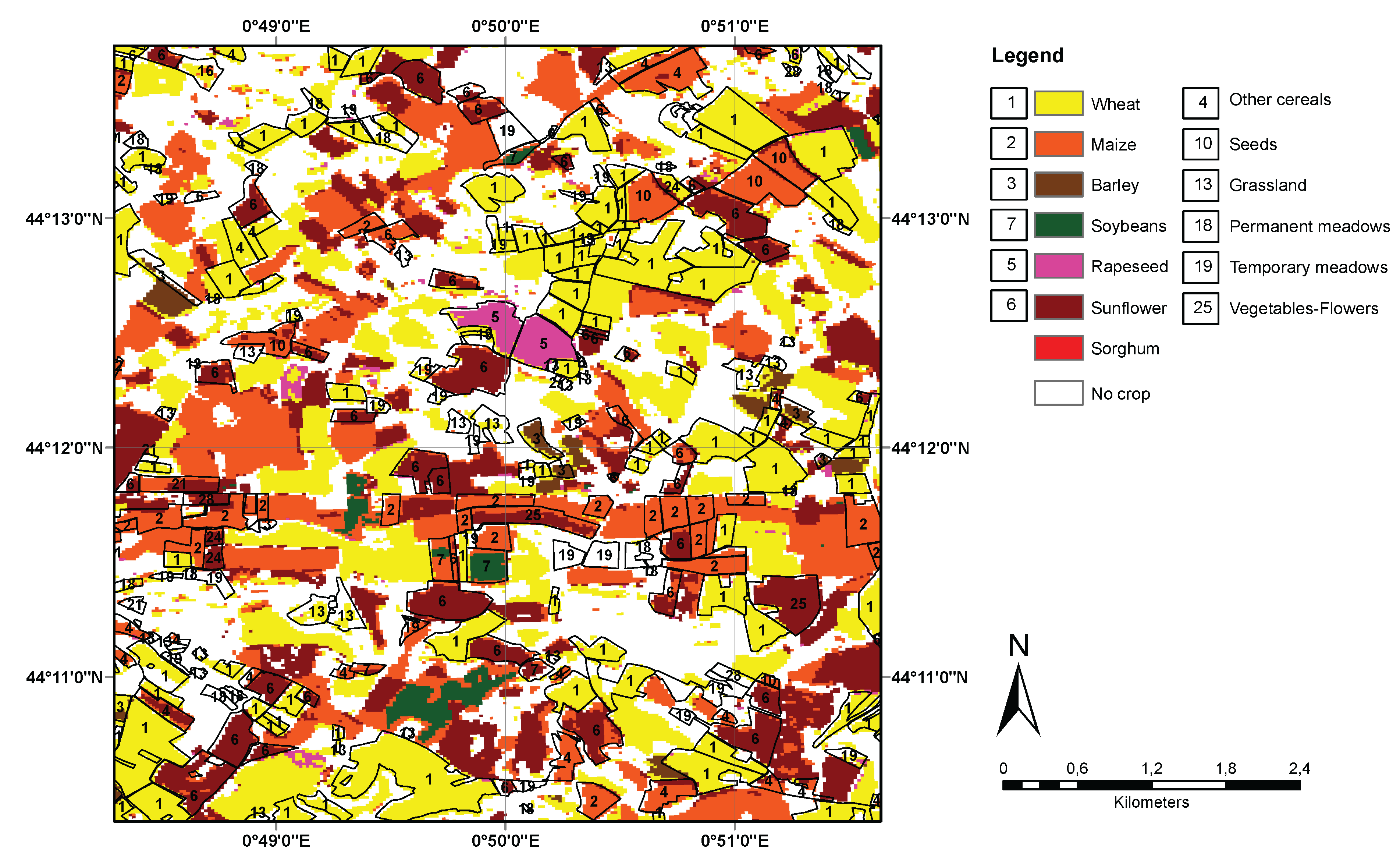
• France (0.570392E, 43.628161N, 16,903 km${}^2$), good: This dataset covers the end of the winter crops and the complete summer crop cycles with more than one image per month, lacking the starting of the winter crops.
• Madagascar (46.987573E, 19.641356S, 14,402 km${}^2$), moderate/bad: Images were taken almost weekly for the middle end of the growing season (from the end of February to the end of April). However, many them have clouds for the eastern half of the image, where the validation data are located.
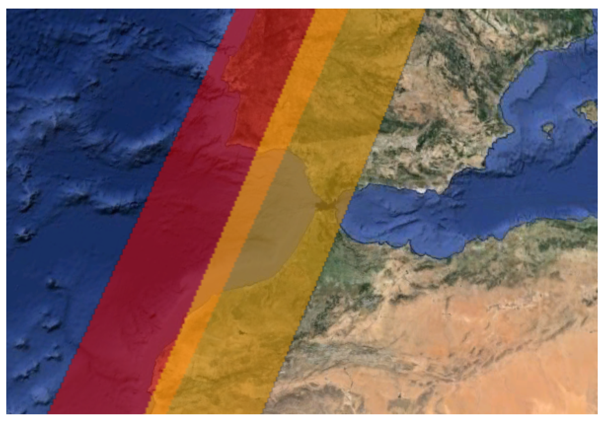
• Morocco (7.858731W, 31.476627N, 14,068 km${}^2$), very good: There was very good coverage from January to June (one image approximately every 5 days).
• Pakistan (72.557226E, 31.477121N, 1199 km${}^2$), bad: The dataset has at least one non-cloudy Landsat in June, one in July, one in September and one in August (June and July with some aerosols). It thus covers the beginning and the end of the growing cycle. There is no acceptable image in the period of the maximum development of the crops.
• Russia (37.917387E, 53.388181N, 3577 km${}^2$), bad: Because of the presence of clouds, there were no SPOT4 (Take5) or Landsat images available. In order to keep the test site in the benchmarking, RapidEye imagery was used covering the middle end of the summer crops from the end of April to July. Only 4 images were free of clouds.
• South Africa (26.577359E, 27.381934S, 2905 km${}^2$), good: Field data correspond to summer crops. The dataset provides good coverage with a good image every week, except for the beginning of the cycle (December/January).
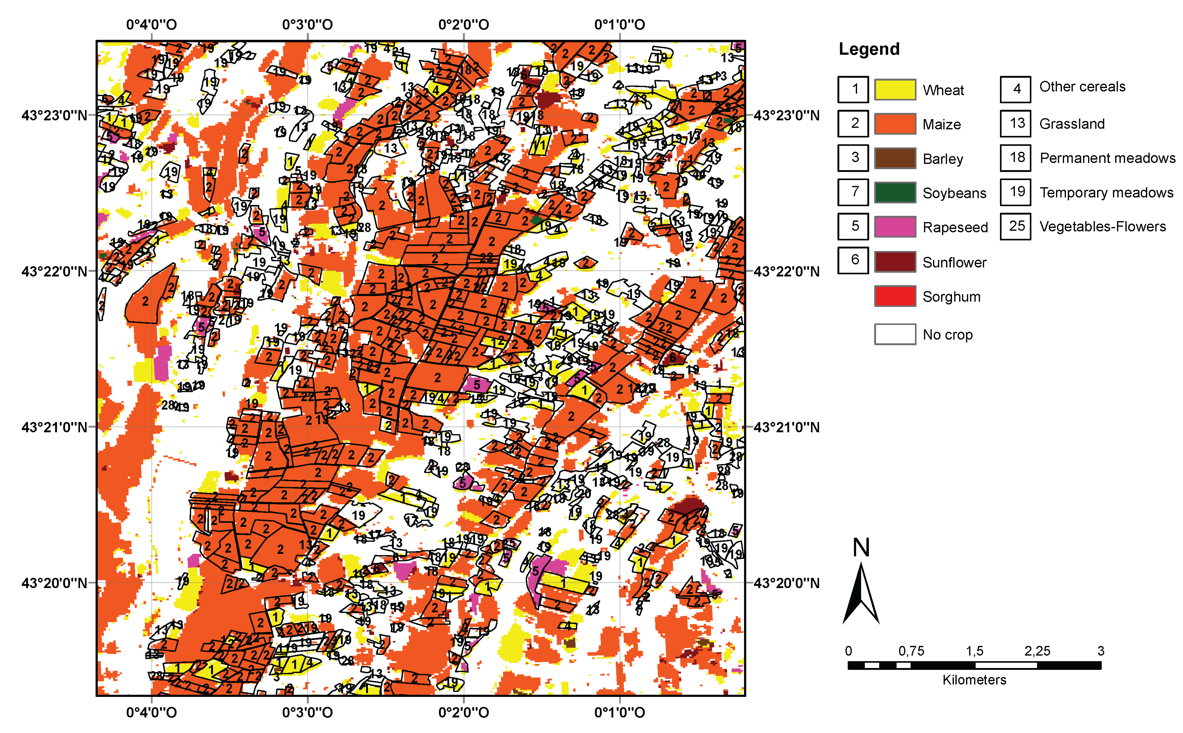
• Ukraine (30.008751E, 50.060014N, 3593 km${}^2$), moderate: April, May and June are covered, which corresponds to the end of the winter crops and the beginning of the summer crops. From December to March, there is no image due to clouds.
• USA (112.168445W, 33.027932N, 5450 km${}^2$), good: There is approximately one image every 5 days from February to June, covering the middle end of the winter and the beginning to middle cycle of the summer crops. Some Landsat data complete the summer cycle with less frequency.

Tables S1–S12 in the Supplementary Information provide the full list of images available.

2.1.2. In Situ Data

Added to the satellite imagery, crop type in situ data were made available by site managers (most of the sites belong to the JECAM network).

Except for Belgium and the USA (where official Land Cover databases were available for 2013), the cropland data were obtained by field observations during the main growing season of the year 2013. Non-cropland classes were also requested in order to have a complete dataset allowing a proper validation of the cropland products. These last data were obtained either from field observations or from institutional data.

The amount of data and the number of crop classes in the nomenclature varies from site to site. The choice of the final nomenclature for each site was made to ensure that the main crops of every site were included.

The main crop types are defined as those covering a minimum area of 5% of the annual cropland and for which the cumulative area reaches more than 75% of the annual cropland in the region. The idea behind these 5% and 75% thresholds is to avoid crop types that represented a too low proportion of the surface. On the one hand, these parcels are most likely to be badly classified. On the other hand, the cost of field campaigns to get enough calibration/validation data would be too high.

The 5% and 75% values come from a detailed analysis of both FAO national cropland statistics and Sentinel-2 for agriculture sites statistics (from land cover maps and/or in situ data). They seem to be a good trade-off to avoid crops that cover a very small surface in the area while, at the same time, maintaining a significant representativeness.

Added to this rationale, the 4 key crops defined in the GEO Global Agricultural Monitoring (GEOGLAM [35]) initiative and the Agricultural Market Information System (AMIS [36]) (wheat, maize, rice and soybean) were prioritized whenever possible.

Tables S13–S24 in the Supplementary Information summarize the crop type classes and the corresponding surfaces available in the in situ data.

2.2. Experiment Design

In this section, we justify the choice of the classification approach, we present the problem of the image time series temporal resampling, we detail the experimental setup and we present the quality metrics used to assess the results.

2.2.1. Strategy Selection

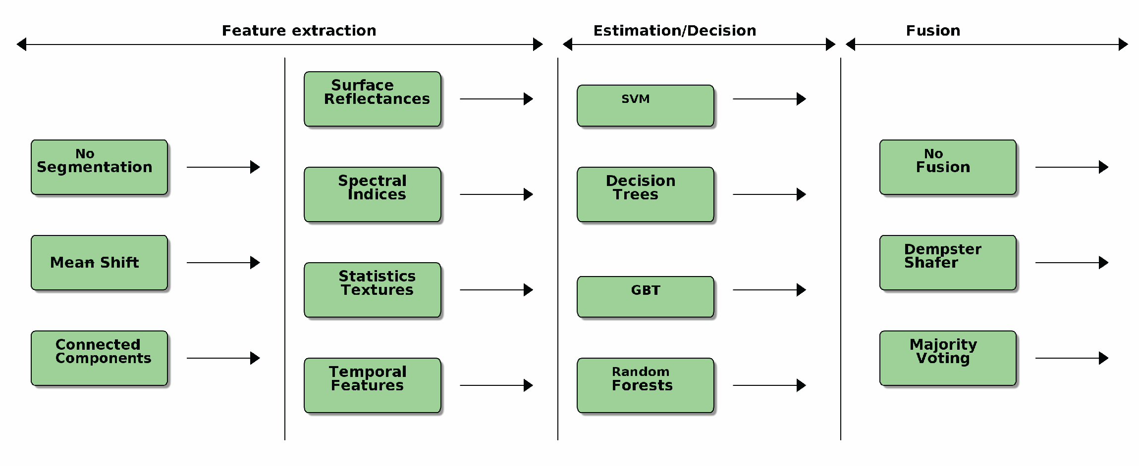
Choice of the Classification Approach

A typical processing chain for land cover map production consists of a sequence of the following processing steps:

• image segmentation in the case of a region-based approach,
• feature extraction,
• classification,
• fusion or post-processing.

For each one of these steps, several algorithmic choices are possible (Figure 1): the segmentation algorithm (depending on the types of fields, for instance), the types of features extracted (spectral, statistical, textural, temporal), the classification algorithm (supervised or unsupervised, kernel based, Bayesian, ensemble classifier), etc.

Figure 1. Choices of algorithms leading to strategy comparisons.

Figure 1. Choices of algorithms leading to strategy comparisons.

The goal of this work is to set up a single processing chain that will operate with good performances on all different sites. Therefore, the best combination of processing steps has to be selected. Since the number of possible combinations is very high, it is unfeasible to evaluate them all on every available test site. On the other hand, a selection of strategies only based on a literature survey is difficult, since most of the published works focus on a single step of the processing chain or compare strategies in very specific settings.

For instance, Duro et al. [37] showed that even for SPOT5 HRG imagery (10 m), there is no statistically-significant advantage to the use of object-based image analysis for agricultural landscapes and that the differences between support vector machines and random forests are not significant either. On the other hand, Rodríguez Galiano et al. [38] showed that random forests are easier to set up and do not suffer from over-learning.

In order to confront some of these findings, a first exploratory phase was set up. This exploratory phase was aimed at evaluating a high number of combinations of the processing steps listed above and at defining the appropriate ranges for the values of the parameters of the different algorithms. For this exploratory phase, only 2 test sites were used. France and Morocco were selected, as they offered the best combination of available images and in situ data.

In terms of algorithms, only the feature extraction and classification steps were studied. The classifiers used were: support vector machines (SVM [39]), decision trees (DT [40]), gradient boosted trees (GBT [41]) and random forests (RF [42]).

The implementation of the selected algorithms we used is the one available in the Orfeo Toolbox [43] free software library.

Using metrics, such as the κ coefficient, the overall accuracy [44] and the F-score [45] (see Section 2.2.3), the classifiers listed above were compared on two test sites. A large set of features, including surface reflectances, normalized radiometric indices (NDVI and other similar band combinations) were run through feature selection approaches. Furthermore, several approaches for dealing with cloudy pixels were applied (no particular processing, using cloud masks as input features, linear and cubic spline interpolation of cloudy data).

The analysis of the results of this exploratory phase can be summarized as follows:

• Segmentation approaches were difficult to be tuned automatically for different kinds of crops and fields, resulting in errors. It was therefore decided not to use a segmentation algorithm, but rather to use the edge-preserving smoothing filtering of the first phase of the mean-shift approach [46].
• The best trade-off between accuracy and processing time for dealing with cloudy data was to perform a temporal linear interpolation of cloudy pixels. There was no improvement in terms of classification metrics using the cubic spline interpolation.
• The most pertinent features for the classification (and therefore used for all of the experiments reported in this paper) were the surface (TOC) reflectances, the NDVI, the NDWI [47] and the brightness (defined as the Euclidean norm of the surface reflectances).
• The classifiers yielding the best performances were the random forests, followed by the gradient boosted trees and then the SVM with a RBFkernel. RF and GBT being similar approaches, only RF and SVM were selected for the benchmarking on the complete set of test sites.

Temporal Resampling

When processing very large areas, even with Sentinel-2 images having a swath of nearly 300 km, several satellite tracks will be needed. The orbital cycle of the satellite results in adjacent tracks being acquired at different dates (+7 days for Sentinel-2; see Figure 2). Combined with the effects of clouds, the observation dates of close regions observed on adjacent orbits may largely differ. This heterogeneous temporal sampling makes the design of an operational land cover map production complex, as training different classifiers for different tracks may introduce artifacts at the boundaries between tracks, both in terms of continuity, but also in terms of classification accuracy.

Figure 2. Example of Sentinel-2 tracks: in red, the acquisitions of Day D; in yellow, those of Day D + 7 (with one satellite) or Day D + 2 (with 2 satellites). Background image ${}^{\copyright }$2015 Google Imagery.

Figure 2. Example of Sentinel-2 tracks: in red, the acquisitions of Day D; in yellow, those of Day D + 7 (with one satellite) or Day D + 2 (with 2 satellites). Background image ${}^{\copyright }$2015 Google Imagery.

One way of overcoming this issue is to resample all image tracks on the same temporal grid. Since the image reflectances already need to be interpolated in order to fill the gaps resulting from clouds, shadows and other artifacts, this resampling can be performed together with the interpolation, which limits the computational cost.

The temporal resampling is implemented as follows. A temporal grid starting with the first acquisition date and with a 5-day sampling step is defined. For every pixel, the time series of each spectral band is linearly interpolated using only the valid data (cloud-free, non-shadow, non-saturated pixels). A new time series is produced selecting the linearly-interpolated values at the dates of the 5-day temporal grid.

The temporal interpolation modifies the observations and may introduce errors, which result in a decreased accuracy of the classifications. The impact of this temporal resampling was therefore assessed in this study as follows: the image time series for each site was resampled on a 5-day period time grid with an offset of 3 days with respect to the real acquisition dates of the SPOT4 (Take5) experiment. The 3-day shift is the worst case, and therefore, an upper bound of the error was estimated. The accuracies of the crop type maps for the original time series and the resampled one were then compared in order to evaluate the impact of the resampling (see Section 3.2).

Final List of Strategies

The result of the exploratory phase allowed narrowing down the list of supervised classifiers to 2, validating the use of the linear gap-filling of the time series and choosing the input image features to be used. The full benchmark on the 12 sites could therefore focus on the comparison of the 2 selected classifiers and the impact of the smoothing and the temporal resampling described above.

The fusion of the output of the 2 selected classifiers was also evaluated. The objective of this evaluation was to assess the complementarity of the results of the 2 classifiers. The fusion approach used was the Dempster–Shafer rule [48] using the confusion matrices (see Section 2.2.3) for the estimation of the masses of belief [49].

The final list of 5 strategies to be benchmarked on the 12 test sites was:

• Random forest classifier;
• SVM classifier with an RBF kernel;
• Dempster–Shafer fusion of the previous approaches;
• Best classifier with a mean-shift smoothing;
• Best classifier with a temporal regular resampling.

2.2.2. Experimental Setup

Figure 3 illustrates the procedure implemented for the assessment of the crop type map production chain.

Figure 3. Block diagram of the crop type map production.

Figure 3. Block diagram of the crop type map production.

The data preparation consists of the following steps:

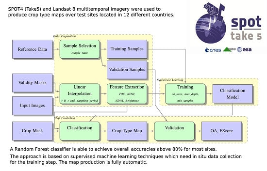
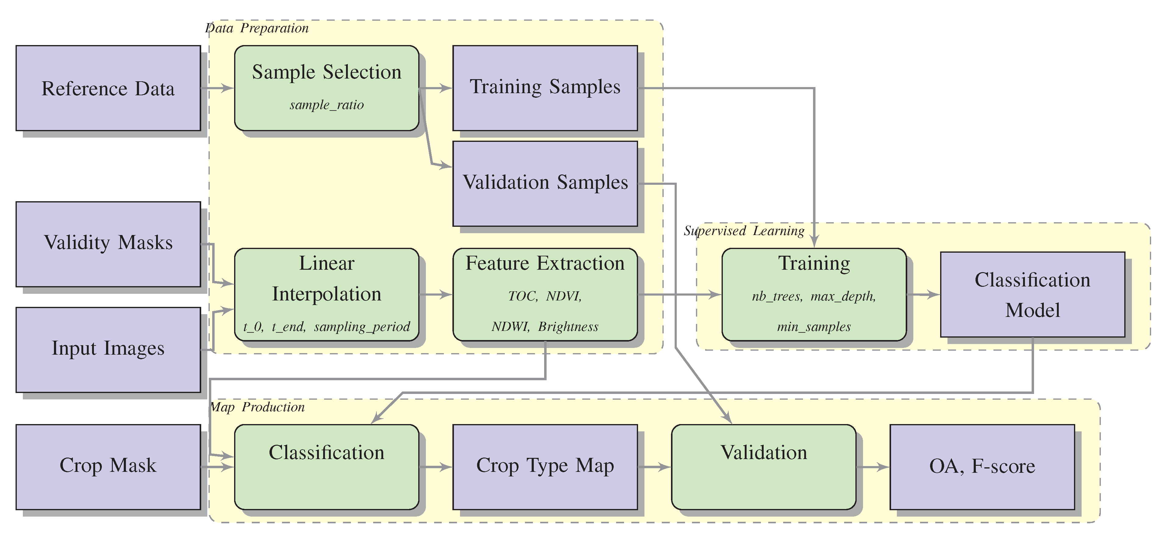
• The reference in situ data are split into 2 disjoint sets of polygons, one for training the classifier and the other for the validation of the produced maps. The split is made at the polygon level in order to ensure that there are no pixels from the same field in the training and the validation sets.
• The validity masks and the input surface reflectance images are used in order to produce a gap-filled time series using linear interpolation of the missing values. In the case of the temporal resampling, all time points are linearly interpolated. The optional smoothing step is applied at this stage.
• The gap-filled time series is used to compute the spectral indices (NDVI, NDWI and brightness) for each acquisition date, which are afterwards stacked with the surface reflectances in order to produce the input features for the classifier.

The training samples (pixel coordinates and associated class labels) are used to train the classifier. The result of this step is the classification model.

The validation is made as follows:

• The input features (time series of reflectances and spectral indices) and the crop mask (The crop mask is another of the Sentinel-2 Agriculture Project products and is assumed to be available here. It consists of a binary mask of cropland areas. The crop type classification is performed only inside the cropland areas.) are used with the classification model in order to produce the crop type map.
• The validation samples are used to produce a confusion matrix for the generated crop type map. The overall accuracy and the F-score per class are computed (see Section 2.2.3 for the details of these metrics). This validation is performed at the pixel level.

The procedure is repeated 10 times with different random draws from the samples in order to estimate confidence intervals and the statistical significance of the performances of the different configurations.

2.2.3. Quality Metrics

>From the confusion matrix, the overall accuracy (OA) and the F-score are computed [50]. The OA is used to evaluate the global performances for each site. Since for some sites, the surfaces covered by each class are not balanced, the F-score of the main class and the minimum F-score for all classes are also studied.

Since every statistic is evaluated several times with different sets of training data, confidence intervals for the statistics can be computed. Only the 95% confidence intervals for the OA will be presented for the sake of brevity. It is worth noting that these confidence intervals have to be computed using a T distribution ([51] p. 302, [52] p. 184) and not a normal distribution, as suggested by Foody in [53], since the number of samples is smaller than 30 (10 random draws in our case).

The quality acceptance thresholds are set to an OA of 50%, with the F-score for the main class higher than 65%.

3. Results and Discussion

As explained in Section 2.2.1, the benchmarking over the full 12 sites was performed using two classifiers (random forests and SVM with an RBF kernel). The assessment of the impact of temporal resampling was also performed as explained above. Finally, the spatial smoothing and the Dempster–Shafer fusion were studied.

3.1. Classifier Comparison

Table 1 presents a summary of the OA results obtained on the 12 test sites. As one can see, OA values are above 0.8 for seven sites, and only three of them are under 0.7. The confidence intervals are very narrow (below 3% for all sites except three of them). Table 2 summarizes the F-score results. F-score values of the main class are also very good for most of the sites. Madagascar is a particular case where most of the test fields are smaller than the pixel size. The case of Burkina Faso is discussed below. Even the minimum F-score of all classes for a given site is acceptable for most of the sites, with only values lower than 0.44 for the cases where image availability and quality were low or where very difficult classes (mixes of crops in Morocco) were present.

Table 1. Results for random forests and SVM. OA with 95% confidence intervals. Bold typeface is used to highlight statistically-significant differences between the two classifiers.

Site	OA	SVM
	Random Forests
Argentina	0.904 ± 0.026	0.898 ± 0.024
Belgium	0.822 ± 0.001	0.642 ± 0.020
Burkina Faso	0.524 ± 0.018	0.335 ± 0.025
China	0.927 ± 0.010	0.876 ± 0.039
France	0.904 ± 0.004	0.857 ± 0.012
Madagascar	0.502 ± 0.058	0.338 ± 0.085
Morocco	0.879 ± 0.005	0.694 ± 0.024
Pakistan	0.727 ± 0.035	0.605 ± 0.045
Russia	0.668 ± 0.019	0.618 ± 0.030
South Africa	0.908 ± 0.011	0.904 ± 0.023
Ukraine	0.752 ± 0.025	0.753 ± 0.018
USA	0.913 ± 0.005	0.905 ± 0.008

Table 1. Results for random forests and SVM. OA with 95% confidence intervals. Bold typeface is used to highlight statistically-significant differences between the two classifiers.

Site	OA	SVM
	Random Forests
Argentina	0.904 ± 0.026	0.898 ± 0.024
Belgium	0.822 ± 0.001	0.642 ± 0.020
Burkina Faso	0.524 ± 0.018	0.335 ± 0.025
China	0.927 ± 0.010	0.876 ± 0.039
France	0.904 ± 0.004	0.857 ± 0.012
Madagascar	0.502 ± 0.058	0.338 ± 0.085
Morocco	0.879 ± 0.005	0.694 ± 0.024
Pakistan	0.727 ± 0.035	0.605 ± 0.045
Russia	0.668 ± 0.019	0.618 ± 0.030
South Africa	0.908 ± 0.011	0.904 ± 0.023
Ukraine	0.752 ± 0.025	0.753 ± 0.018
USA	0.913 ± 0.005	0.905 ± 0.008

Table 2. Results for random forests and SVM. F-score of the main class and minimum F-score of all classes. Bold typeface is used to highlight statistically-significant differences between the two classifiers.

Site	Random Forests	Minimum	SVM	Minimum
	Main Class		Main Class
Argentina	0.9399	0.7586	0.9374	0.7304
Belgium	0.8735	0.6886	0.7030	0.4818
Burkina Faso	0.7266	0.0553	0.4800	0.0961
China	0.9616	0.4455	0.9270	0.4032
France	0.9310	0.5250	0.8977	0.5582
Madagascar	0.0488	0.0402	0.1526	0.1526
Morocco	0.9326	0.2734	0.7938	0.3680
Pakistan	0.8107	0.1326	0.7210	0.2212
Russia	0.8435	0.2237	0.8119	0.2041
South Africa	0.9542	0.3941	0.9469	0.4293
Ukraine	0.8589	0.5493	0.8608	0.6211
USA	0.9382	0.6859	0.9368	0.6849

Table 2. Results for random forests and SVM. F-score of the main class and minimum F-score of all classes. Bold typeface is used to highlight statistically-significant differences between the two classifiers.

Site	Random Forests	Minimum	SVM	Minimum
	Main Class		Main Class
Argentina	0.9399	0.7586	0.9374	0.7304
Belgium	0.8735	0.6886	0.7030	0.4818
Burkina Faso	0.7266	0.0553	0.4800	0.0961
China	0.9616	0.4455	0.9270	0.4032
France	0.9310	0.5250	0.8977	0.5582
Madagascar	0.0488	0.0402	0.1526	0.1526
Morocco	0.9326	0.2734	0.7938	0.3680
Pakistan	0.8107	0.1326	0.7210	0.2212
Russia	0.8435	0.2237	0.8119	0.2041
South Africa	0.9542	0.3941	0.9469	0.4293
Ukraine	0.8589	0.5493	0.8608	0.6211
USA	0.9382	0.6859	0.9368	0.6849

For the sake of brevity, only three sites are presented in detail here. The choice of these three sites is made in order to cover an ideal case (France, with good results and a large number of classes), an intermediate case (Ukraine, with medium quality image time series, satisfactory results, important number of classes) and a case with bad results (Burkina Faso, difficult landscape, bad imagery). For these three sites, the quality of the in situ data was also correct, although in the case of Burkina Faso, the reference polygons have surfaces of only a few pixels.

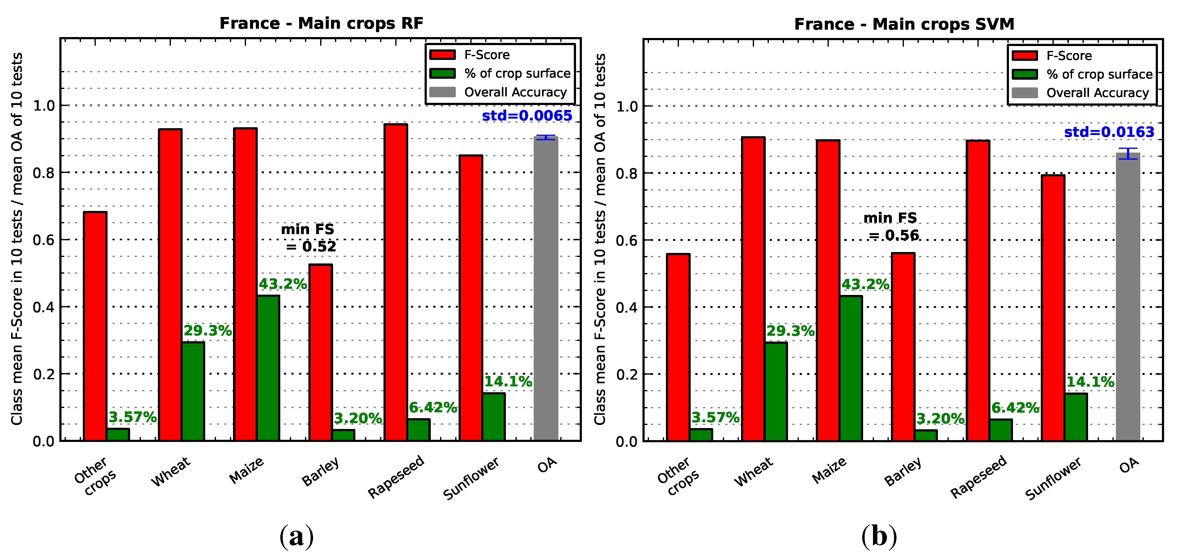
3.1.1. France

The main crops covering 75% of the crop surface according to the FAO statistics are wheat, maize, barley, rapeseed and sunflower, which coincide with the main crops of the in situ data.

The individual results (see Figure 4) of the main crops are satisfactory, except for barley. This class is also under-represented in the in situ data, and the confusion of this class with wheat is high. This is a classic confusion, as both crops have nearly identical phenological cycles and spectral responses.

Table 3 and Table 4 show the confusion matrices for RF and SVM, respectively.

Figure 4. F-score and OA results for RF and SVM for the France test site. (a) RF; (b) SVM.

Figure 4. F-score and OA results for RF and SVM for the France test site. (a) RF; (b) SVM.

Table 3. Confusion matrix for RF on the France test site.

Class	Wheat	Maize	Barley	Rapeseed	Sunflower	Other Crops
Wheat	24,061	486	122	72	84	4
Maize	809	35,105	1	14	751	127
Barley	1440	21	920	21	9	0
Rapeseed	317	108	18	5018	42	3
Sunflower	345	1777	24	8	10,008	30
Other Crops	19	1044	0	0	358	1692

Table 3. Confusion matrix for RF on the France test site.

Class	Wheat	Maize	Barley	Rapeseed	Sunflower	Other Crops
Wheat	24,061	486	122	72	84	4
Maize	809	35,105	1	14	751	127
Barley	1440	21	920	21	9	0
Rapeseed	317	108	18	5018	42	3
Sunflower	345	1777	24	8	10,008	30
Other Crops	19	1044	0	0	358	1692

Table 4. Confusion matrix for SVM on the France test site.

Class	Wheat	Maize	Barley	Rapeseed	Sunflower	Other Crops
Wheat	21,536	524	1893	594	178	112
Maize	951	31,027	98	273	2786	1671
Barley	804	9	1498	110	15	9
Rapeseed	212	78	172	4971	26	35
Sunflower	210	1446	130	111	9654	683
Other Crops	17	570	11	7	440	2049

Table 4. Confusion matrix for SVM on the France test site.

Class	Wheat	Maize	Barley	Rapeseed	Sunflower	Other Crops
Wheat	21,536	524	1893	594	178	112
Maize	951	31,027	98	273	2786	1671
Barley	804	9	1498	110	15	9
Rapeseed	212	78	172	4971	26	35
Sunflower	210	1446	130	111	9654	683
Other Crops	17	570	11	7	440	2049

The classification produced by the RF classifier based on field surveys made by our teams was also compared to the RPG (Registre Parcellaire Graphique) database, which corresponds to the farmers’ declaration of their cultivated areas. This comparison allowed evaluating the results in areas far from the in situ data location. For this comparison, the nomenclature of the RPG (with more classes than the one of the benchmarking) was used.

Figure 5 and Figure 6 show the results of the crop type map with the RPG polygons overlayed. The image of Figure 5 corresponds to an area located about 40 km north of the area where the in situ data were collected. The image of Figure 6 corresponds to an area with a higher altitude close to the Pyrenees mountain range.

Figure 5. Comparison of the crop map type obtained using the RF classifier and field surveys with the RPG database in a region 40 km north to the field data collection site. Numbers indicate the crop type in the reference data and colors correspond to the output of the classifier.

Figure 5. Comparison of the crop map type obtained using the RF classifier and field surveys with the RPG database in a region 40 km north to the field data collection site. Numbers indicate the crop type in the reference data and colors correspond to the output of the classifier.

Figure 6. Comparison of the crop map type obtained using the RF classifier and field surveys with the Registre Parcellaire Graphique (RPG) database on a high altitude region far from the field data collection site. Numbers indicate the crop type in the reference data, and colors correspond to the output of the classifier.

Figure 6. Comparison of the crop map type obtained using the RF classifier and field surveys with the Registre Parcellaire Graphique (RPG) database on a high altitude region far from the field data collection site. Numbers indicate the crop type in the reference data, and colors correspond to the output of the classifier.

A confusion matrix was also calculated using RPG polygons as a reference dataset. All of the comparable classes have F-score values higher than 0.7 excluding barley, which has the lowest value (0.48). The OA was 0.8.

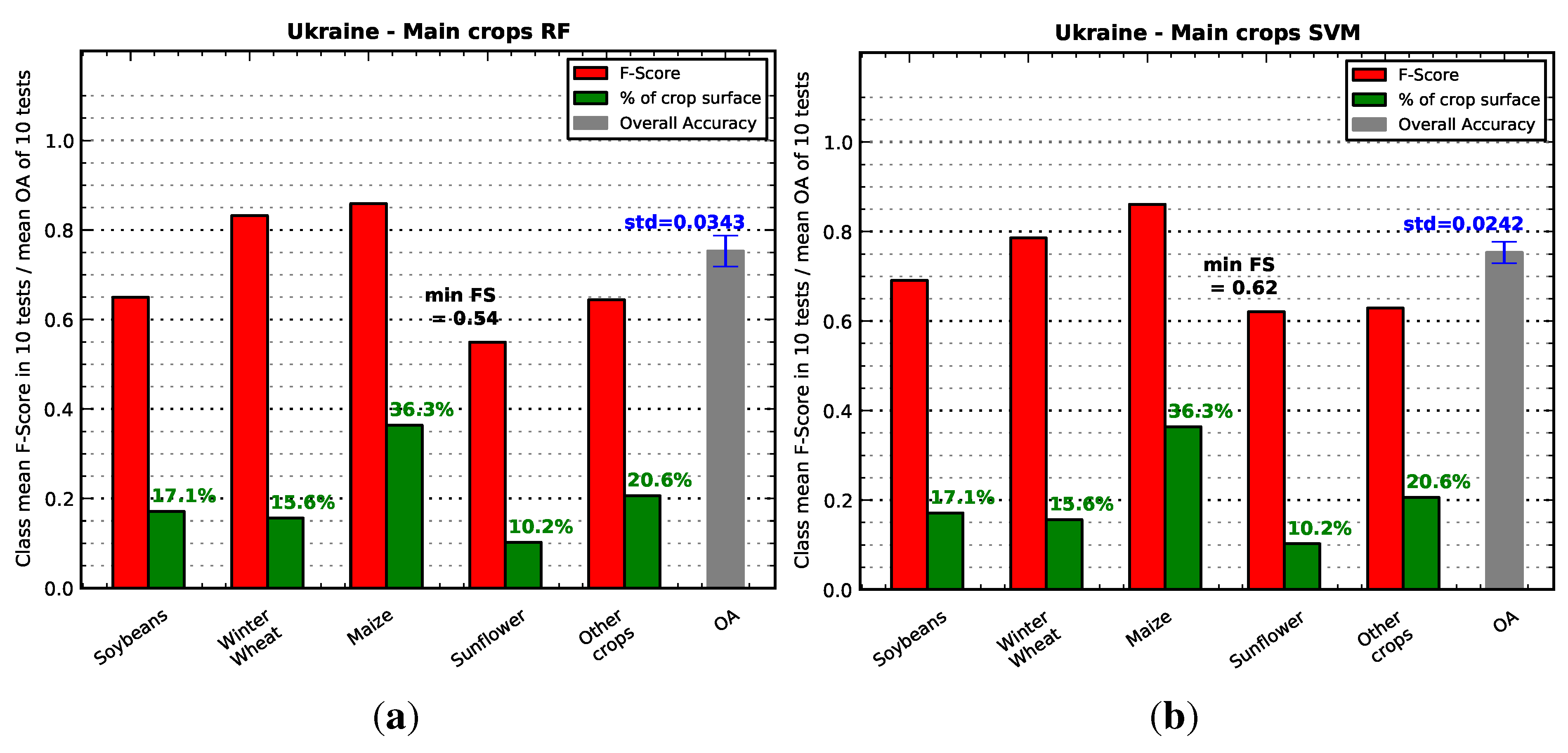
3.1.2. Ukraine

The main crops according to the FAO statistics (wheat, sunflower, maize, barley and potatoes) are all present in the in situ dataset. However, potatoes and barley represent less than 2% of the total cropland surface. As soybean is a main crop within the five main crops of the in situ dataset, it was included in the final legend (maize, soybean, wheat, sunflower).

Figure 7 presents the results for the two classifiers.

>From February to March, the site is covered by snow, and during the summer season, after June, the cloud coverage is high, which results in only a good coverage of the end of the winter crops and the start of the summer crops.

Some explanations of the previous results can be found by analyzing the detailed confusion matrices (Table 5 and Table 6 for RF and SVM, respectively). Samples of winter wheat are indeed correctly classified, but confusion with other classes (spring wheat, spring barley, other cereals) is present. Maize is also well classified, but other summer crops (soybeans, sunflower) are also classified as this class.

Figure 7. F-score and OA results for RF and SVM for the Ukraine test site. (a) RF; (b) SVM.

Figure 7. F-score and OA results for RF and SVM for the Ukraine test site. (a) RF; (b) SVM.

Table 5. Confusion matrix for RF on the Ukraine test site.

Class	Maize	Soybeans	Winter Wheat	Sunflower	Other Crops
Maize	53,662	2741	44	626	312
Soybeans	8127	19,476	188	1465	1460
Winter Wheat	89	100	26,702	59	2003
Sunflower	3577	3868	171	8426	2724
Other Crops	2538	3162	7896	1020	19,225

Table 5. Confusion matrix for RF on the Ukraine test site.

Class	Maize	Soybeans	Winter Wheat	Sunflower	Other Crops
Maize	53,662	2741	44	626	312
Soybeans	8127	19,476	188	1465	1460
Winter Wheat	89	100	26,702	59	2003
Sunflower	3577	3868	171	8426	2724
Other Crops	2538	3162	7896	1020	19,225

Table 6. Confusion matrix for SVM on the Ukraine test site.

Class	Maize	Soybeans	Winter Wheat	Sunflower	Other Crops
Maize	52,811	3575	69	1014	893
Soybeans	6166	21,706	382	1810	1248
Winter Wheat	50	164	24,429	80	4490
Sunflower	2683	3957	183	10,168	1987
Other Crops	2494	2788	7896	746	19,655

Table 6. Confusion matrix for SVM on the Ukraine test site.

Class	Maize	Soybeans	Winter Wheat	Sunflower	Other Crops
Maize	52,811	3575	69	1014	893
Soybeans	6166	21,706	382	1810	1248
Winter Wheat	50	164	24,429	80	4490
Sunflower	2683	3957	183	10,168	1987
Other Crops	2494	2788	7896	746	19,655

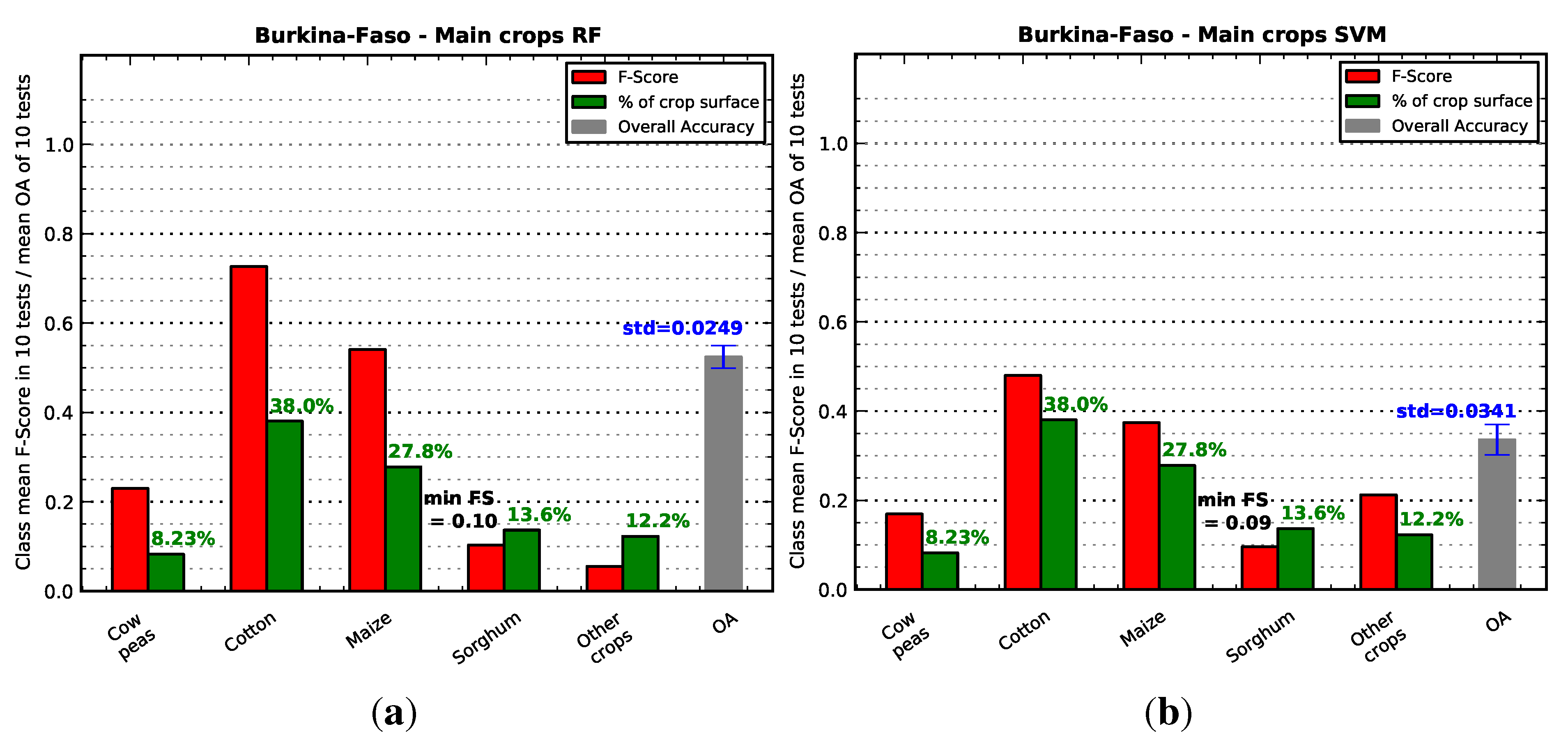
3.1.3. Burkina Faso

All of the main crops according to the FAO statistics (sorghum, cow peas, millet and maize) are represented in the in situ data; however, the millet class represented less than 1.5% of the reference cropland area, and it was not included in the final legend. On the other hand, cotton was included, since it amounted to 38% of the in situ dataset. Figure 8 summarizes the results for the two classifiers.

Figure 8. F-score and OA results for RF and SVM for the Burkina Faso test site. (a) RF; (b) SVM.

Figure 8. F-score and OA results for RF and SVM for the Burkina Faso test site. (a) RF; (b) SVM.

Table 7 and Table 8 show the confusion matrices for RF and SVM, respectively.

Table 7. Confusion matrix for RF on the Burkina test site.

Class	Maize	Sorghum	Cow Peas	Cotton	Other Crops
Maize	155	21	3	56	1
Sorghum	62	9	3	38	1
Cow Peas	30	9	12	21	1
Cotton	44	10	3	262	0
Other Crops	48	11	15	25	3

Table 7. Confusion matrix for RF on the Burkina test site.

Class	Maize	Sorghum	Cow Peas	Cotton	Other Crops
Maize	155	21	3	56	1
Sorghum	62	9	3	38	1
Cow Peas	30	9	12	21	1
Cotton	44	10	3	262	0
Other Crops	48	11	15	25	3

Table 8. Confusion matrix for SVM on the Burkina test site.

Class	Maize	Sorghum	Cow Peas	Cotton	Other Crops
Maize	108	25	11	21	68
Sorghum	44	10	10	12	39
Cow Peas	21	4	12	6	32
Cotton	103	24	15	115	1
Other Crops	30	7	18	7	39

Table 8. Confusion matrix for SVM on the Burkina test site.

Class	Maize	Sorghum	Cow Peas	Cotton	Other Crops
Maize	108	25	11	21	68
Sorghum	44	10	10	12	39
Cow Peas	21	4	12	6	32
Cotton	103	24	15	115	1
Other Crops	30	7	18	7	39

Only Landsat 8 images were used in this site, which was not among the SPOT4 (Take5) sites, and the available dates barely cover the growing season going from June to October. From May to July and in September, only one image per month was available, and no image was available in August.

A particularity of this site is its agro-forestry crop system. Trees are present in cultivated fields, as they offer a number of benefits for the annual crops. In addition to that, there is also intra-plot variability due to the small-scale farming. Figure 9 shows some polygons of the field data overlaid on a QuickBird satellite image of 3 May 2013. As one can observe, the polygons that correspond to agricultural units are highly heterogeneous and therefore difficult to classify as a unique crop.

Figure 9. Intra-plot variability in the Burkina Faso site. In situ data plots are overlayed in red. The fields are highly heterogeneous and difficult to classify as a single crop. ${}^{\copyright }$2015 Google Imagery, ${}^{\copyright }$2015 DigitalGlobe.

Figure 9. Intra-plot variability in the Burkina Faso site. In situ data plots are overlayed in red. The fields are highly heterogeneous and difficult to classify as a single crop. ${}^{\copyright }$2015 Google Imagery, ${}^{\copyright }$2015 DigitalGlobe.

3.2. Temporal Resampling

In order to evaluate the impact on the temporal resampling on the crop type mapping quality, 10 classifications using different random draws for the polygons used for the training were performed for each site, both with and without temporal resampling, as described in Section 2.2.1.

Table 9 presents the summary of the results for the OA. The OA original values differ from those of Table 1 because the “other crops” classes were not regrouped for this analysis. As one can observe, the mean values for the OA over the 10 draws are very similar between both configurations for all sites, showing a very slight decrease in quality for the case where the temporal resampling is used. The large p-values obtained indicate that for all sites, except South Africa and Ukraine, the differences are not statistically significant (p-values should be smaller than 0.05).

Table 9. Assessment of the effect of the temporal resampling for each site. Overall accuracy with the 95% confidence interval without and with temporal resampling and p-value of the t-test of the related sets of samples.

Site	OA	OA	p-Value
	Original	Resampled
Argentina	0.904 ± 0.026	0.893 ± 0.028	0.120
Belgium	0.816 ± 0.001	0.816 ± 0.001	0.312
Burkina Faso	0.522 ± 0.018	0.503 ± 0.018	0.122
China	0.927 ± 0.010	0.911 ± 0.031	0.193
France	0.904 ± 0.004	0.905 ± 0.004	0.770
Madagascar	0.501 ± 0.058	0.498 ± 0.070	0.818
Morocco	0.876 ± 0.004	0.875 ± 0.009	0.771
Pakistan	0.727 ± 0.035	0.723 ± 0.036	0.684
Russia	0.665 ± 0.019	0.665 ± 0.019	0.947
South Africa	0.907 ± 0.011	0.894 ± 0.015	0.023
Ukraine	0.740 ± 0.025	0.724 ± 0.024	0.019
U.S.-Maricopa	0.911 ± 0.006	0.911 ± 0.006	0.939

Table 9. Assessment of the effect of the temporal resampling for each site. Overall accuracy with the 95% confidence interval without and with temporal resampling and p-value of the t-test of the related sets of samples.

Site	OA	OA	p-Value
	Original	Resampled
Argentina	0.904 ± 0.026	0.893 ± 0.028	0.120
Belgium	0.816 ± 0.001	0.816 ± 0.001	0.312
Burkina Faso	0.522 ± 0.018	0.503 ± 0.018	0.122
China	0.927 ± 0.010	0.911 ± 0.031	0.193
France	0.904 ± 0.004	0.905 ± 0.004	0.770
Madagascar	0.501 ± 0.058	0.498 ± 0.070	0.818
Morocco	0.876 ± 0.004	0.875 ± 0.009	0.771
Pakistan	0.727 ± 0.035	0.723 ± 0.036	0.684
Russia	0.665 ± 0.019	0.665 ± 0.019	0.947
South Africa	0.907 ± 0.011	0.894 ± 0.015	0.023
Ukraine	0.740 ± 0.025	0.724 ± 0.024	0.019
U.S.-Maricopa	0.911 ± 0.006	0.911 ± 0.006	0.939

These results allow us to adopt temporal resampling of the image time series in order to use the same set of virtual dates over very large areas.

3.3. Smoothing and Fusion

The impact of the smoothing as a pre-processing step was also evaluated, but the results were not conclusive due to the use of 20-m (SPOT4) and 30-m (Landsat 8) resolution images. Indeed, the spatial resolution of the images has a strong impact on the effects of the quality of the segmentation and 20 m and 30 m are too low of resolutions to be compared to the 10-m resolution of the visible bands of Sentinel-2. Therefore, these results will not be presented here, and further analysis will be carried on in the future with both SPOT5 imagery (the Take5 experiment will take place again from April to September 2015 during the end of life of the SPOT5 satellite) and Sentinel-2 data when available.

The Dempster–Shafer fusion yielded a minor improvement only in Madagascar and Burkina Faso and resulted in decreased OA values for many other sites, with respect to the results yielded by the best classifier.

4. Conclusions

This paper has presented a thorough work of benchmarking a processing chain for the production of crop type land cover maps. The assessment of the performances of the proposed chain has been performed on 12 test sites spread all over the globe presenting different landscapes, crops and agricultural practices.

For most of the sites, the obtained results are compatible with an operational (with no human operation, except the reference data collection and in compliance with the accuracy specifications) production at the country scale. The computational cost depends on the number of crop classes and the number of available images. The average processing time of the sites presented here including training and map production was 0.65 s per km${}^2$ on a computer with 24 Intel${}^{\circledR }$ Xeon${}^{\circledR }$ CPUs at 3.07 GHz and 64 GB of RAM. This would result in 120 h for a whole country the size of France.

Some sites presented low mapping qualities due to two main causes: the quality of the available imagery and the difficulty of mapping some crop systems. The first issue will probably be solved by the improved spatial and temporal resolutions provided by Sentinel-2. The second issue will need further research and development.

The same processing chain was used for all sites, and the operational software will be distributed by ESA as free and open source software. The current prototype used for the work presented in this paper is already available [54]. The quantitative assessment of the results indicate that the random forest classifier operating on linearly-interpolated time series yields the best results.

Sentinel-2 will be operational at the beginning of 2016. It will significantly improve the observational capabilities for agricultural monitoring in terms of temporal and spatial resolution. Synergy with Landsat 8 observations will nevertheless always be beneficial and in many cases necessary for fulfilling the user requirements in terms of crop type mapping. This possibility has already been demonstrated in this study, where SPOT4 (Take5) and Landsat 8 were jointly used to produce crop type maps.

Sentinel-2 will certainly bring improvements in the results thanks to the enhanced spatial resolution and the increased number of spectral bands, mainly in the red-edge spectrum. It will therefore be interesting to evaluate the usefulness of object-oriented approaches, the use of textures and the use of other spectral indices.

References

- Foley, J.A.; Ramankutty, N.; Brauman, K.A.; Cassidy, E.S.; Gerber, J.S.; Johnston, M.; Mueller, N.D.; O’Connell, C.; Ray, D.K.; West, P.C.; et al. Solutions for a Cultivated Planet. Nature 2011, 478, 337–342. [Google Scholar] [CrossRef] [PubMed]
- Godfray, H.C.J.; Beddington, J.R.; Crute, I.R.; Haddad, L.; Lawrence, D.; Muir, J.F.; Pretty, J.; Robinson, S.; Thomas, S.M.; Toulmin, C. Food Security: The Challenge of Feeding 9 Billion People. Science 2010, 327, 812–818. [Google Scholar] [CrossRef] [PubMed]
- Rounsevell, M.; Ewert, F.; Reginster, I.; Leemans, R.; Carter, T. Future Scenarios of European Agricultural Land Use. Agric. Ecosyst. Environ. 2005, 107, 117–135. [Google Scholar] [CrossRef]
- Searchinger, T.; Heimlich, R.; Houghton, R.A.; Dong, F.; Elobeid, A.; Fabiosa, J.; Tokgoz, S.; Hayes, D.; Yu, T.H. Use of US Croplands for Biofuels Increases Greenhouse Gases through Emissions from Land-Use Change. Science 2008, 319, 1238–1240. [Google Scholar] [CrossRef] [PubMed]
- Green, R.E.; Cornell, S.J.; Scharlemann, J.P.W.; Balmford, A. Farming and the Fate of Wild Nature. Science 2005, 307, 550–555. [Google Scholar] [CrossRef] [PubMed]
- Tilman, D. Forecasting Agriculturally Driven Global Environmental Change. Science 2001, 292, 281–284. [Google Scholar] [CrossRef] [PubMed]
- Benayas, J.M.R.; Bullock, J.M. Restoration of Biodiversity and Ecosystem Services on Agricultural Land. Ecosystems 2012, 15, 883–899. [Google Scholar] [CrossRef] [Green Version]
- Schwilch, G.; Bestelmeyer, B.; Bunning, S.; Critchley, W.; Herrick, J.; Kellner, K.; Liniger, H.; Nachtergaele, F.; Ritsema, C.; Schuster, B.; et al. Experiences in Monitoring and Assessment of Sustainable Land Management. Land Degrad. Dev. 2010, 22, 214–225. [Google Scholar] [CrossRef]
- Drusch, M.; Bello, U.D.; Carlier, S.; Colin, O.; Fernandez, V.; Gascon, F.; Hoersch, B.; Isola, C.; Laberinti, P.; Martimort, P.; et al. Sentinel-2: Esa’s Optical High-Resolution Mission for Gmes Operational Services. Remote Sens. Environ. 2012, 120, 25–36. [Google Scholar] [CrossRef]
- Sentinel-2 for Agriculture. Available online: http://www.esa-sen2agri.org/ (accessed on 18 September 2015).
- Committee on Earth Observation Satellites. CEOS Acquisition Strategy for GEOGLAM Phase 1. Available online: http://ceos.org/document_management/Ad_Hoc_Teams/GEOGLAM/GEOGLAM_CEOS-Acquisition-Strategy-for-GEOGLAM-Phase-1_Nov2013.pdf (accessed on 18 September 2015).
- JECAM. Available online: http://www.jecam.org/ (accessed on 18 September 2015).
- Hagolle, O.; Sylvander, S.; Huc, M.; Claverie, M.; Clesse, D.; Dechoz, C.; Lonjou, V.; Poulain, V. SPOT4 (Take5): Simulation of Sentinel-2 Time Series on 45 Large sites. Remote Sens. 2015. Accept. [Google Scholar]
- Roy, D.; Wulder, M.; Loveland, T.; Woodcock, C.E.; Allen, R.; Anderson, M.; Helder, D.; Irons, J.; Johnson, D.; Kennedy, R.; et al. Landsat-8: Science and Product Vision for Terrestrial Global Change Research. Remote Sens. Environ. 2014, 145, 154–172. [Google Scholar] [CrossRef]
- Salmon, J.; Friedl, M.A.; Frolking, S.; Wisser, D.; Douglas, E.M. Global Rain-Fed, Irrigated, and Paddy Croplands: A New High Resolution Map Derived From Remote Sensing, Crop Inventories and Climate Data. Int. J. Appl. Earth Obs. Geoinf. 2015, 38, 321–334. [Google Scholar] [CrossRef]
- Fritz, S.; See, L.; McCallum, I.; You, L.; Bun, A.; Moltchanova, E.; Duerauer, M.; Albrecht, F.; Schill, C.; Perger, C.; et al. Mapping Global Cropland and Field Size. Glob. Chang. Biol. 2015, 21, 1980–1992. [Google Scholar] [CrossRef] [PubMed] [Green Version]
- Defourny, P.; Vancutsem, C.; Bicheron, P.; Brockmann, C.; Nino, F.; Schouten, L.; Leroy, M. GlobCover: A 300 m global land cover product for 2005 using ENVISAT MERIS time series. In Proceedings of the ISPRS Commission VII Symposium Remote Sensing: From Pixels to Processes, Enschede, The Netherlands, 8–11 May 2006.
- Friedl, M.A.; Sulla-Menashe, D.; Tan, B.; Schneider, A.; Ramankutty, N.; Sibley, A.; Huang, X. MODIS Collection 5 global land cover: Algorithm refinements and characterization of new datasets, 2001-2012, Collection 5.1 IGBP Land Cover. Boston University: Boston, MA, USA.
- Townshend, J.R.; Masek, J.G.; Huang, C.; Vermote, E.F.; Gao, F.; Channan, S.; Sexton, J.O.; Feng, M.; Narasimhan, R.; Kim, D.; et al. Global Characterization and Monitoring of Forest Cover Using Landsat Data: Opportunities and Challenges. Int. J. Digit. Earth 2012, 5, 373–397. [Google Scholar] [CrossRef]
- Whitcraft, A.; Becker-Reshef, I.; Justice, C. A Framework for Defining Spatially Explicit Earth Observation Requirements for a Global Agricultural Monitoring Initiative (GEOGLAM). Remote Sens. 2015, 7, 1461–1481. [Google Scholar] [CrossRef]
- Whitcraft, A.; Becker-Reshef, I.; Killough, B.; Justice, C. Meeting Earth Observation Requirements for Global Agricultural Monitoring: An Evaluation of the Revisit Capabilities of Current and Planned Moderate Resolution Optical Earth Observing Missions. Remote Sens. 2015, 7, 1482–1503. [Google Scholar] [CrossRef]
- Banskota, A.; Kayastha, N.; Falkowski, M.J.; Wulder, M.A.; Froese, R.E.; White, J.C. Forest Monitoring Using Landsat Time Series Data: A Review. Can. J. Remote Sens. 2014, 40, 362–384. [Google Scholar] [CrossRef]
- Badhwar, G. Classification of Corn and Soybeans Using Multitemporal Thematic Mapper Data. Remote Sens. Environ. 1984, 16, 175–181. [Google Scholar] [CrossRef]
- Murthy, C.S.; Raju, P.V.; Badrinath, K.V.S. Classification of Wheat Crop with Multi-Temporal Images: Performance of Maximum Likelihood and Artificial Neural Networks. Int. J. Remote Sens. 2003, 24, 4871–4890. [Google Scholar] [CrossRef]
- Brown, J.C.; Kastens, J.H.; Coutinho, A.C.; de Castro Victoria, D.; Bishop, C.R. Classifying multiyear agricultural land use data from Mato Grosso using time-series MODIS vegetation index data. Remote Sens. Environ. 2013, 130, 39–50. [Google Scholar] [CrossRef]
- Wardlow, B.D.; Egbert, S.L. Large-area crop mapping using time-series MODIS 250 m NDVI data: An assessment for the U.S. Central Great Plains. Remote Sens. Environ. 2008, 112, 1096–1116. [Google Scholar] [CrossRef]
- Lobell, D.B.; Asner, G.P. Cropland distributions from temporal unmixing of MODIS data. Remote Sens. Environ. 2004, 93, 412–422. [Google Scholar] [CrossRef]
- Ozdogan, M. The spatial distribution of crop types from MODIS data: Temporal unmixing using Independent Component Analysis. Remote Sens. Environ. 2010, 114, 1190–1204. [Google Scholar] [CrossRef]
- Verbeiren, S.; Eerens, H.; Piccard, I.; Bauwens, I.; Orshoven, J.V. Sub-Pixel Classification of Spot-Vegetation Time Series for the Assessment of Regional Crop Areas in Belgium. Int. J. Appl. Earth Observ. Geoinf. 2008, 10, 486–497. [Google Scholar]
- Hansen, M.C.; Egorov, A.; Roy, D.P.; Potapov, P.; Ju, J.; Turubanova, S.; Kommareddy, I.; Loveland, T.R. Continuous Fields of Land Cover for the Conterminous United States Using Landsat Data: First Results From the Web-Enabled Landsat Data (weld) Project. Remote Sens. Lett. 2011, 2, 279–288. [Google Scholar] [CrossRef]
- Zhong, L.; Gong, P.; Biging, G.S. Efficient Corn and Soybean Mapping with Temporal Extendability: A Multi-Year Experiment Using Landsat Imagery. Remote Sens. Environ. 2014, 140, 1–13. [Google Scholar] [CrossRef]
- Wu, B.; Gommes, R.; Zhang, M.; Zeng, H.; Yan, N.; Zou, W.; Zheng, Y.; Zhang, N.; Chang, S.; Xing, Q.; et al. Global Crop Monitoring: A Satellite-Based Hierarchical Approach. Remote Sensing 2015, 7, 3907–3933. [Google Scholar] [CrossRef]
- Theia Land Data Centre. Available online: https://www.theia-land.fr/en/products/spot4-take5 (accessed on 18 September 2015).
- Centre d’Etudes Spatiales de la BIOsphere. Available online: http://www.cesbio.ups-tlse.fr/ (accessed on 18 September 2015).
- Geoglam crop monitor. Available online: http://www.geoglam-crop-monitor.org/index.php (accessed on 18 September 2015).
- AMIS. Available online: http://www.amis-outlook.org (accessed on 18 September 2015).
- Duro, D.C.; Franklin, S.E.; Dubé, M.G. A Comparison of Pixel-Based and Object-Based Image Analysis with Selected Machine Learning Algorithms for the Classification of Agricultural Landscapes Using Spot-5 Hrg Imagery. Remote Sens. Environ. 2012, 118, 259–272. [Google Scholar] [CrossRef]
- Rodriguez-Galiano, V.; Ghimire, B.; Rogan, J.; Chica-Olmo, M.; Rigol-Sanchez, J. An Assessment of the Effectiveness of a Random Forest Classifier for Land-Cover Classification. ISPRS J. Photogramm. Remote Sens. 2012, 67, 93–104. [Google Scholar] [CrossRef]
- Burges, C.J. A tutorial on support vector machines for pattern recognition. Data Min. Knowl. Discov. 1998, 2, 121–167. [Google Scholar] [CrossRef]
- Breiman, L.; Friedman, J.; Olshen, R.; Stone, C. Classification and Regression Trees; Taylor and Francis: New York, NY, USA.
- Friedman, J.H. Greedy function approximation: A gradient boosting machine. Ann. Stat. 2001, 29, 1189–1232. [Google Scholar] [CrossRef]
- Breiman, L. Random forests. Mach. Learn. 2001, 45, 5–32. [Google Scholar] [CrossRef]
- Orfeo Toolbox. Available online: http://www.orfeo-toolbox.org/ (accessed on 18 September 2015).
- Congalton, R.G. A review of assessing the accuracy of classifications of remotely sensed data. Remote Sens. Environ. 1991, 37, 35–46. [Google Scholar] [CrossRef]
- Powers, D.M. Evaluation: From Precision, Recall and F-Measure to ROC, Informedness, Markedness and Correlation. J. Mach. Lear. Technol. 2011, 1, 37–63. [Google Scholar]
- Commaniciu, D. Mean Shift: A Robust Approach toward Feature Space Analysis. IEEE Trans. Pattern Anal. Mach. Intell. 2002, 24, 603–619. [Google Scholar] [CrossRef]
- Gao, B.C. NDWI. A normalized difference water index for remote sensing of vegetation liquid water from space. Remote Sens. Environ. 1996, 58, 257–266. [Google Scholar] [CrossRef]
- Smets, P. What is Dempster-Shafer’s model? In Advances in the Dempster-Shafer Theory of Evidence; John Wiley & Sons, Inc.: New York, NY, USA, 1994; pp. 5–34. [Google Scholar]
- Xu, L.; Krzyzak, A.; Suen, C.Y. Methods of Combining Multiple Classifiers and Their Applications To Handwriting Recognition. IEEE Trans. Syst. Man Cybern. 1992, 22, 418–435. [Google Scholar] [CrossRef]
- Sokolova, M.; Lapalme, G. A Systematic Analysis of Performance Measures for Classification Tasks. Inf. Process. Manag. 2009, 45, 427–437. [Google Scholar] [CrossRef]
- Klemens, B. Modeling with Data: Tools and Techniques for Scientific Computing; Princeton University Press: Princeton, NJ, USA, 2008. [Google Scholar]
- Jackson, S. Research Methods and Statistics: A Critical Thinking Approach; Cengage Learning: Boston, MA, USA, 2015. [Google Scholar]
- Foody, G.M. Classification Accuracy Comparison: Hypothesis Tests and the Use of Confidence Intervals in Evaluations of Difference, Equivalence and Non-Inferiority. Remote Sens. Environ. 2009, 113, 1658–1663. [Google Scholar] [CrossRef]
- Processing Chain for Crop type Map Production. Available online: http://tully.ups-tlse.fr/ariasm/croptype_bench/ (accessed on 18 September 2015).
© 2015 by the authors; licensee MDPI, Basel, Switzerland. This article is an open access article distributed under the terms and conditions of the Creative Commons Attribution license (http://creativecommons.org/licenses/by/4.0/).
Share and Cite
Inglada, J.; Arias, M.; Tardy, B.; Hagolle, O.; Valero, S.; Morin, D.; Dedieu, G.; Sepulcre, G.; Bontemps, S.; Defourny, P.; et al. Assessment of an Operational System for Crop Type Map Production Using High Temporal and Spatial Resolution Satellite Optical Imagery. Remote Sens. 2015, 7, 12356-12379. https://doi.org/10.3390/rs70912356
Inglada J, Arias M, Tardy B, Hagolle O, Valero S, Morin D, Dedieu G, Sepulcre G, Bontemps S, Defourny P, et al. Assessment of an Operational System for Crop Type Map Production Using High Temporal and Spatial Resolution Satellite Optical Imagery. Remote Sensing. 2015; 7(9):12356-12379. https://doi.org/10.3390/rs70912356
Chicago/Turabian StyleInglada, Jordi, Marcela Arias, Benjamin Tardy, Olivier Hagolle, Silvia Valero, David Morin, Gérard Dedieu, Guadalupe Sepulcre, Sophie Bontemps, Pierre Defourny, and et al. 2015. "Assessment of an Operational System for Crop Type Map Production Using High Temporal and Spatial Resolution Satellite Optical Imagery" Remote Sensing 7, no. 9: 12356-12379. https://doi.org/10.3390/rs70912356