Automated Ortho-Rectification of UAV-Based Hyperspectral Data over an Agricultural Field Using Frame RGB Imagery

Abstract

Low-cost Unmanned Airborne Vehicles (UAVs) equipped with consumer-grade imaging systems have emerged as a potential remote sensing platform that could satisfy the needs of a wide range of civilian applications. Among these applications, UAV-based agricultural mapping and monitoring have attracted significant attention from both the research and professional communities. The interest in UAV-based remote sensing for agricultural management is motivated by the need to maximize crop yield. Remote sensing-based crop yield prediction and estimation are primarily based on imaging systems with different spectral coverage and resolution (e.g., RGB and hyperspectral imaging systems). Due to the data volume, RGB imaging is based on frame cameras, while hyperspectral sensors are primarily push-broom scanners. To cope with the limited endurance and payload constraints of low-cost UAVs, the agricultural research and professional communities have to rely on consumer-grade and light-weight sensors. However, the geometric fidelity of derived information from push-broom hyperspectral scanners is quite sensitive to the available position and orientation established through a direct geo-referencing unit onboard the imaging platform (i.e., an integrated Global Navigation Satellite System (GNSS) and Inertial Navigation System (INS). This paper presents an automated framework for the integration of frame RGB images, push-broom hyperspectral scanner data and consumer-grade GNSS/INS navigation data for accurate geometric rectification of the hyperspectral scenes. The approach relies on utilizing the navigation data, together with a modified Speeded-Up Robust Feature (SURF) detector and descriptor, for automating the identification of conjugate features in the RGB and hyperspectral imagery. The SURF modification takes into consideration the available direct geo-referencing information to improve the reliability of the matching procedure in the presence of repetitive texture within a mechanized agricultural field. Identified features are then used to improve the geometric fidelity of the previously ortho-rectified hyperspectral data. Experimental results from two real datasets show that the geometric rectification of the hyperspectral data was improved by almost one order of magnitude.

1. Introduction

Precision agriculture has become an important activity for: (1) optimizing crop yield given diminishing resources; (2) increasing the reliability of crop-yield prediction; and (3) reducing the agricultural impact on the environment through efficient use of fertilizers and pesticides [1]. Technologies are also being adapted for advanced plant breeding where phenotypic data are obtained to quantify plant growth, structure and composition at multiple scales over the growing season [2]. Traditional phenotyping has primarily been conducted in field-based plots, which is time-consuming, labor-intensive and includes destructive sampling. Phenotypic data are also acquired in research environments via proximal sensing in controlled environments, such as greenhouses and growth rooms, which unfortunately are restricted in both extent and capability to emulate field-based conditions. Thus, phenotyping is a significant bottleneck in advancing plant breeding. Novel phenotyping techniques, which can be utilized to acquire relevant data over extended areas, are crucial [2,3]. Remote sensing systems onboard satellite, airborne and wheel-based platforms can play an important role in high throughput phenotyping. With the ever-increasing technological developments in Mobile Mapping Systems (MMS) on different platforms, remote sensing-based phenotyping has become an attractive option [4]. Improved performance of integrated Global Navigation Satellite Systems (GNSS) and Inertial Navigation Systems (INS) together with the reduced cost of imaging sensors operating in different portions of the electromagnetic spectrum are among the main reasons for the growing interest in MMS for high throughput phenotyping. Among the possible MMS platforms, UAVs are now becoming competitive platforms for remotesensing-based phenotyping, as they can be easily and cost-effectively deployed while collecting geospatial data with higher temporal and spatial resolution than other platforms [5,6,7,8]. Thus, UAVs equipped with directly geo-referenced imaging sensors are also being used for these applications [9].

To obtain a rich set of structure and chemistry-based traits, the UAV platforms are being equipped with RGB cameras and hyperspectral scanners. RGB cameras guarantee high geometric resolution for accurate localization and estimation of important plant traits, such as height, canopy closure and leaf structure. Hyperspectral scanners with fine spectral resolution [10,11] provide useful data for the estimation of canopy nitrogen, chlorophyll content and various narrow-band vegetation indices [12,13,14,15,16]. Due to the volume of collected data, in general, RGB cameras implement frame arrays, whereas hyperspectral scanners are most commonly based on a linear array that captures scenes while operating in a push-broom mode (i.e., the scene coverage is achieved through multiple exposures of the linear array during the platform’s motion along its trajectory) [17]. To relate the sensory data from either frame or push-broom imaging systems to spatial locations relative to a desired reference frame, some sort of control is needed to define the datum for the derived information. This control can be established using Ground Control Points (GCPs) and/or the implementation of an integrated GNSS/INS unit onboard the mapping platform. The latter is the preferred option since GNSS/INS-based direct geo-referencing can reduce or even eliminate the need for establishing GCPs, which is quite expensive and operationally impractical for high throughput phenotyping over extended areas. Unfortunately, the endurance and payload constraints are major factors that could impede the deployment of a cost-effective and comprehensive UAV-based phenotyping platform. Therefore, the remote sensing and agricultural communities mainly rely on UAVs equipped with consumer-grade direct geo-referencing and imaging systems, which are relatively small and light weight, providing inaccurate position and orientation information compared to those equipped with survey-grade GNSS/INS units. Modern automated triangulation of overlapping frame imagery can be conducted while using minimal GCPs and/or low-quality navigation information from consumer-grade GNSS/INS units [18]. However, the inherent weaker imaging geometry of push-broom scanners due to their multiple exposures of the linear array during the platform’s motion along its trajectory requires accurate navigation data. A promising approach for improving the geometric fidelity of hyperspectral data while using consumer-grade navigation systems uses frame camera imagery in the scene-to-ground transformation of the hyperspectral-based information.

Few studies focus on the use of frame-based images to improve the geo-referencing information of hyperspectral scanner scenes. Suomalainen et al. [19] compensated for the inferior quality of direct geo-referencing information through simultaneous integration of captured frame images and a Digital Elevation Model (DEM), which was derived from the frame images. Ramirez-Paredes et al. [20] presented a computer-vision approach for the indirect geo-referencing of the hyperspectral scenes, which estimated a set of transformation parameters relating the reference frames of frame and hyperspectral imagery. In [5], a methodology was presented for improving the ortho-rectification of hyperspectral imagery in the presence of low-quality navigation information with the help of frame imagery using tie points and linear features. In this approach, a transformation function is developed to model the impact of residual artifacts in the direct geo-referencing information. The majority of these approaches focus on the derivation of the mathematical transformation function between the reference frames of frame and hyperspectral images. Unfortunately, time-consuming manual efforts are needed to detect tie point/linear features that are used for the estimation of the parameters of the transformation function. Therefore, automated identification of tie features among overlapping frame and hyperspectral imagery is critical to the operational implementation of these approaches.

The photogrammetric and computer vision research communities have investigated the identification of conjugate features in imagery from different sensor modalities. The identification of tie points in high resolution imagery, especially those exhibiting different geometric and spectral characteristics, is mainly established by applying a feature-based approach. First, strong features (e.g., points, lines and possibly regions) are detected. Then, a descriptor is derived for the detected features and used for the identification of conjugate features in overlapping images. Scale-Invariant Feature Transform (SIFT) [21], Speeded-Up Robust Feature (SURF) [22] and Harris corner detectors and descriptors [23] are among the most commonly-used approaches. Feature-based approaches have been implemented for the registration of very high resolution images with the aim of extracting well-distributed tie points [24,25,26,27,28,29,30,31]. Those approaches, however, might have poor performance for scenes acquired over agricultural fields because of the large number of similar features, which are not necessarily conjugate, arising from the repetitive plant patterns.

The objective of this paper is to introduce an automated approach for improving the geometric rectification of hyperspectral images in the presence of low-quality navigation data through the incorporation of frame images. The suggested procedure, which is presented in the remainder of this paper, is based on the following processing framework.

• Manipulate the frame imagery while using minimal control to produce a geometrically-accurate orthophoto, which will be denoted as the RGB-based orthophoto.
• Utilize the low-quality navigation data for ortho-rectifying the hyperspectral data. Since the navigation data are based on a consumer-grade GNSS/INS unit, the rectified scenes will be denoted as partially-rectified hyperspectral orthophotos. In other words, residual errors in the navigation data are expected to have a negative impact on the ortho-rectification process; thus, we use the term “partially-rectified”.
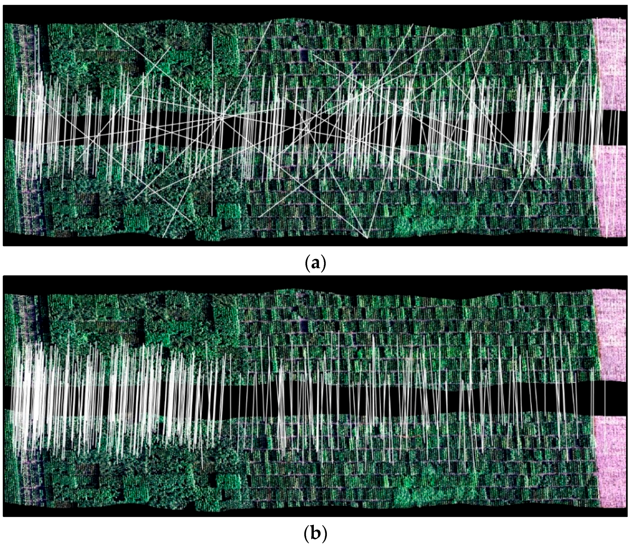
• Develop a matching strategy that relies on the available navigation data to identify conjugate features among the partially-rectified hyperspectral and RGB-based orthophotos to minimize mismatches arising from the repetitive pattern in a mechanized agriculture field.
• Use the matched features to derive the parameters of a transformation function that models the impact of residual errors in the navigation data on the partially-rectified hyperspectral orthophoto.
• Incorporate the transformation parameters in a resampling procedure that transforms the partially-rectified hyperspectral orthophoto to the reference frame of the RGB-based one.

2. Methodology

The proposed methodology is based on the assumption that a consumer-grade GNSS/INS unit has been used to provide the direct geo-referencing information for frame-based and hyperspectral push-broom scanner imagery. Thanks to recent advances in the automated triangulation of frame imagery, photogrammetric processing from an RGB camera can be carried out using minimal control, which could be either in the form of a few GCPs and/or derived from a consumer-grade navigation unit. The geo-referencing parameters together with the DEM are used to produce a geometrically-accurate RGB-based orthophoto. The hyperspectral data together with the DEM and GNSS/INS-based geo-referencing information are also processed to produce a partially-rectified hyperspectral-based orthophoto, which suffers from the impact of residual errors in the push-broom scanner position and orientation information. The geometric fidelity of the partially-rectified hyperspectral orthophoto can be improved through its co-registration with the RGB-based orthophoto. This registration process can be achieved automatically through three main steps: (1) automated identification of conjugate/tie point features among the RGB-based and partially-rectified hyperspectral orthophotos; (2) derivation of a set of parameters that describe the transformation function relating the reference frames of these orthophotos; and (3) resampling the partially-rectified hyperspectral orthophotos to the reference frame of the RGB-based orthophoto.

Due to the limited angular field-of-view of the push-broom hyperspectral scanner, the area of interest is covered through several flight lines with some side lap. In this paper, the automated identification of conjugate points between the RGB-based orthophoto and the partially-rectified hyperspectral orthophotos is facilitated through a two-faceted matching strategy. The first aims at modifying the SURF-based matching of key features to impose constraints that compensate for the fact that the repetitive patterns within the covered area are conducive to establishing false correspondences. The second facet uses the GNSS/INS-based position and orientation information to limit the search space for conjugate features. More specifically, the modified SURF-based matching is used to identify conjugate features among neighboring partially-rectified hyperspectral orthophotos to improve the relative alignment among these rectified scenes. In other words, the matching procedure is used to derive a set of approximate geometric transformation functions among neighboring partially-rectified hyperspectral orthophotos. Then, these approximate transformation functions are used to identify conjugate features among the RGB-based and partially-rectified hyperspectral orthophotos. Finally, the conjugate features are employed to derive the parameters of the transformation function relating the reference frames of these orthophotos. The processing workflow of the proposed procedure is summarized in Figure 1. The remainder of this section covers the modification of the SURF-based feature matching to mitigate the problems arising from having a repetitive pattern within the covered area. Then, we explain how the modified SURF is used to identify conjugate features among the partially-rectified hyperspectral and RGB-based orthophotos. Finally, we introduce the theoretical background for using the identified tie points to derive the parameters of a transformation function that considers the impact of residual errors in the GNSS/INS navigation data on the quality of the derived hyperspectral orthophotos.

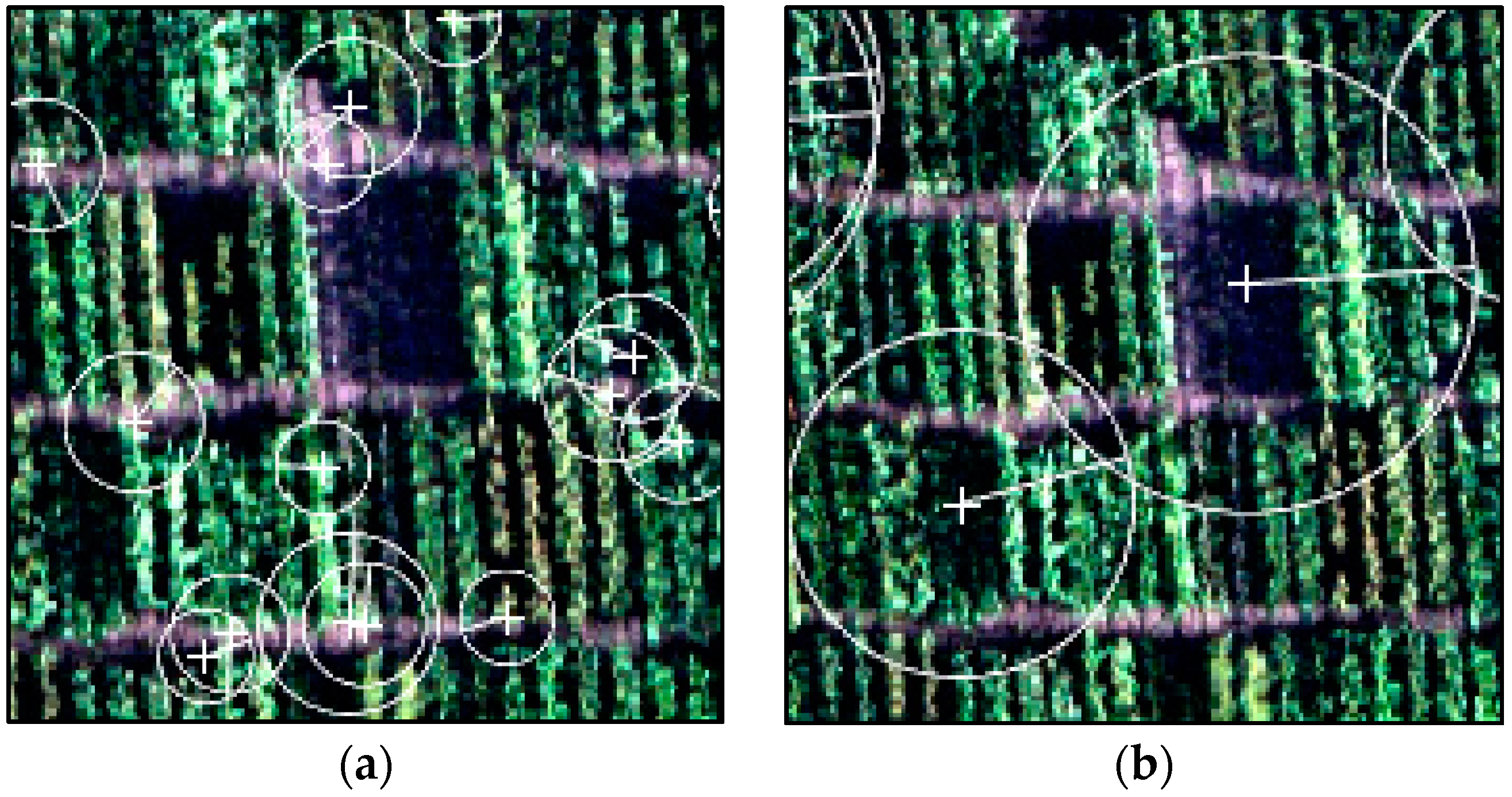
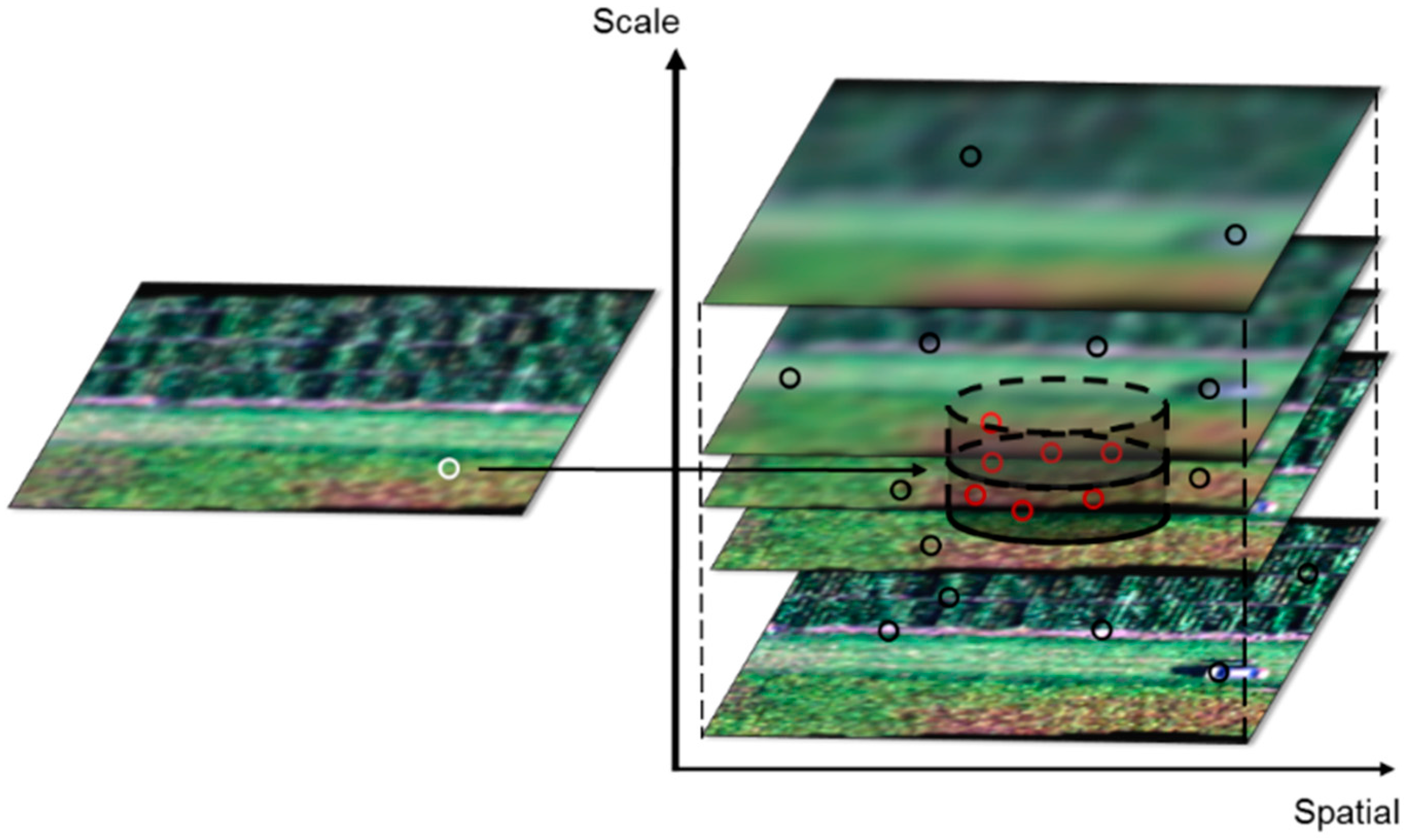
2.1. Speeded-Up Robust Feature Algorithm

This section provides a brief overview of the Speeded-Up Robust Feature (SURF) algorithm [22], which is a scale- and rotation-invariant feature detector and descriptor for identifying corresponding points (i.e., tie points) in overlapping images. These images will be denoted as template and query images. The template is the image where the feature of interest is located. The query image is the overlapping image where we seek to identify features corresponding to the ones in the template. Within the feature detection stage, the SURF algorithm uses a Hessian matrix approximation, which calculates the second-order partial derivative of an image, to locate feature points through the estimated local curvature. SURF constructs a scale space through image convolution with rectangular masks of different sizes. The convolution results in a series of blob response maps at different scales. In contrast to the Scale-Invariant Feature Transform (SIFT) that uses a Gaussian pyramid for constructing the scale space, SURF employs an integral image, which leads to a faster feature detection process [22]. A blob response threshold is applied to select feature points with high-contrast relative to their local neighborhoods. Once the features are detected, 3D non-maximum suppression is performed to identify the location and scale of prominent features with subpixel accuracy. To achieve rotation invariance, the main orientation of detected features is calculated using the sum of all Haar wavelet responses within a circular neighborhood. The detected features thus far are characterized by a 4D vector $\left(x,y,\sigma ,\theta \right)$, where $x$ and $y$ are the location of the feature within the image in question, $\sigma$ is the scale where this feature is defined and $\theta$ is its main orientation. The SURF approach then defines a square region, which has been rotated according to the feature orientation, centered on the detected feature point to generate its descriptor. The elements of the descriptor vector are based on the sums of Haar wavelet responses. Each feature has a 64D descriptor vector, which is used for the identification of conjugate features in overlapping images. In other words, conjugate features in overlapping images are expected to exhibit minimal Euclidean distance between the respective descriptors. For reliable identification of the feature in a query image corresponding to a selected feature in the template image, the minimum Euclidean distance should be significantly smaller than the second shortest distance when considering all of the features in the query image. Therefore, a match will be accepted when the ratio between the minimum and next smallest Euclidean distances is less than a user-defined threshold $T_r$. Additional details related to SURF are contained in [22].

Detected features and their descriptor vectors might not be conducive for the identification of reliable matches in imagery acquired over agricultural fields (refer to Figure 2 that shows an example of a partially-rectified hyperspectral orthophoto from a given flight line where repetitive patterns are quite obvious). Therefore, the SURF-based matching procedure should be adapted to consider the challenging nature of such data. The following paragraph emphasizes some of the characteristics of SURF that could be relevant for improving the reliability of the identification of conjugate features between the partially-rectified hyperspectral and RGB-based orthophotos. It should be noted that the modified SURF algorithm can also be used for scenes without repetitive patterns if direct geo-referencing information (i.e., position and orientation information of the used sensors) and spatial resolution of the considered scenes are known.

One should note that the scale domain defines the scale range within which the feature is detected and described. A feature having a small scale signifies that such a feature and its descriptor vector are derived at a fine resolution while considering a small neighborhood around that feature. A feature having a large scale means that it is defined at a coarse resolution while considering a large neighborhood centered at that feature. Figure 3a illustrates features having a small scale, where the crosshairs denote the locations of the different features, while the circles denote the scale range for defining the respective descriptors. The lines within the circles denote the main orientation of the different features. As can be seen in Figure 3a, derived features at a fine scale are not unique. That is, several features in the query image could have similar descriptors while not being really conjugate to a selected feature in the template image. Features derived at a coarse scale, as can be seen in Figure 3b, have a higher probability of being unique, thus leading to more reliable matches in the presence of repetitive pattern, which is the case for agricultural scenes. Therefore, for reliable matching, one could only consider features having scale values that are larger than a predefined threshold $T_{\sigma }$. To increase the reliability of the matching process, it is usually performed in both forward and backward directions (i.e., by reversing the roles of the template and query images). This process is commonly known as cross-matching. A match is considered correct only if it is accepted by both the forward and backward matching procedures.

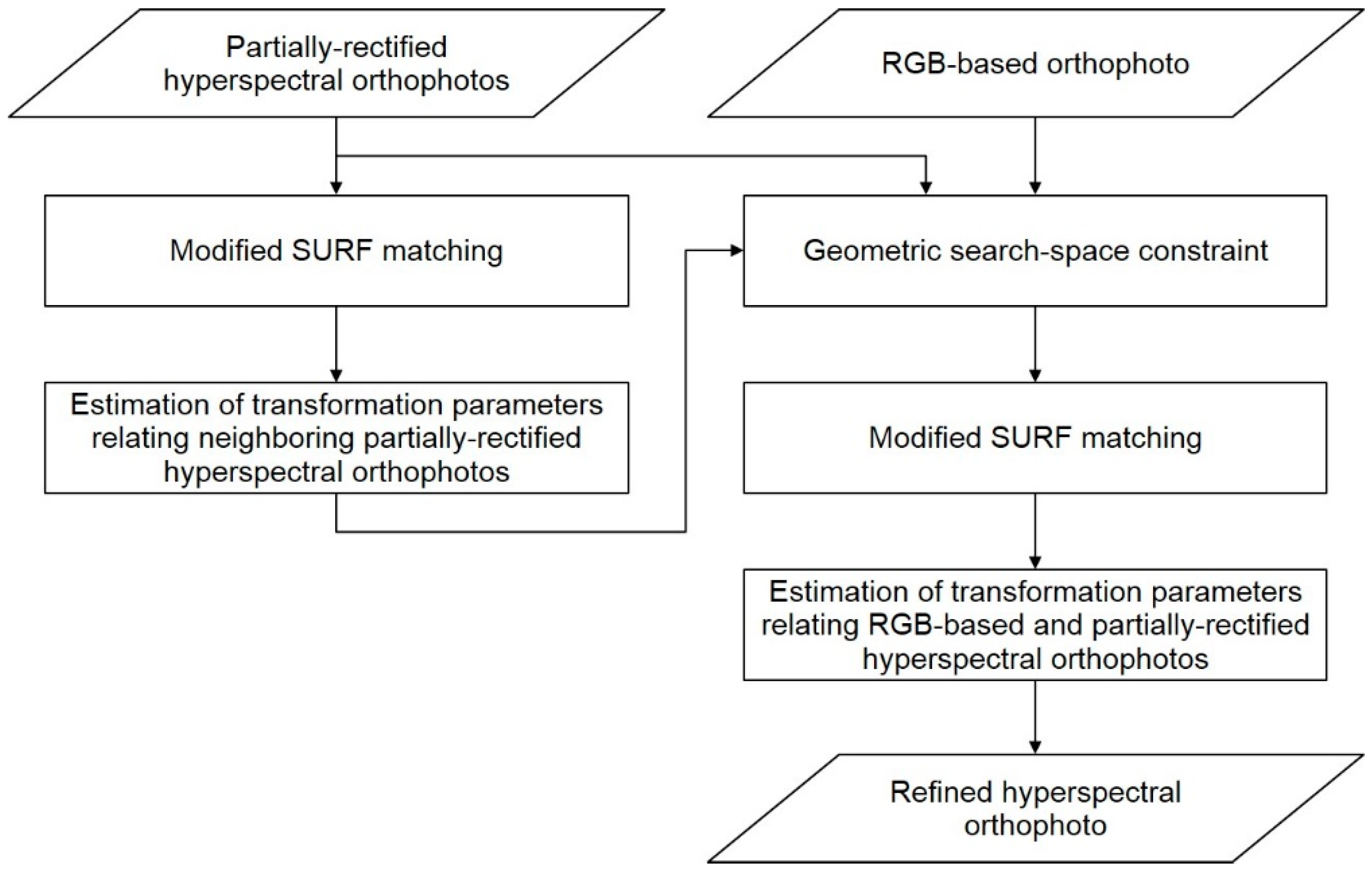
2.2. Modified SURF Algorithm

The generated descriptors for repetitive features observed in row crops might be quite similar to each other, leading to false matching results. We propose to constrain the solution to minimize the probability of wrongly matching non-corresponding features that exhibit similar descriptors by considering the spatial location, scale and main orientation of the detected features.

Regarding the feature location, one should note that even though the GNSS/INS navigation data are not as accurate as needed for this application, the information can be used to filter out improbable matches. We implement a search space, which is commensurate with the quality of the GNSS/INS navigation data, to constrain the spatial extent of the search space for conjugate features in the query image. We also include an orientation constraint because truly corresponding features should exhibit similar orientation (once again, this characteristic is attributed to the fact that we are dealing with partially-rectified data, i.e., the ortho-rectified images are approximately aligned to the GNSS/INS-based reference frame). Finally, the matching process uses the known Ground Sampling Distances (GSDs) in the RGB-based and partially-rectified orthophotos to limit the scale range where conjugate features can be identified. Thus, the SURF-based matching is modified to limit the spatial search space for conjugate features while considering the scale and orientation of potential candidates in the query image. Specifically, rather than simply using the Euclidean distance between the descriptors for the features in the template and query images as the matching criterion, we also use the spatial location, scale and orientation of the detected features. Utilizing the GNSS/INS data to constrain the spatial location of the search space is discussed in Section 2.3. The following paragraphs deal with the orientation and scale consideration for improving the performance of the matching process.

As a result of the repetitive row pattern within a mechanized agriculture field, considering orientation during the descriptor vector generation might lead to truly corresponding features being deemed non-conjugate or vice versa. The feature descriptor is evaluated using a region aligned along the rows and columns of the respective images. Thus, the descriptor vectors are derived while assuming that truly conjugate features should have a similar orientation. As for considering the scale of the feature, we rely on the GSDs of the template and query images. For example, assume that ${\sigma }_i$ and ${\sigma }_j$ are scales of the extracted features $i$ and $j$ from the template and query images, respectively. Feature $j$ in the query image can be considered as a matching candidate to feature $i$ in the template image if the constraint in Equation (1) is satisfied.

$$T_s\le \frac{GS{D}_q{\sigma }_i}{GS{D}_t{\sigma }_j}\le \frac{1}{T_s}$$

(1)

where $T_s$ denotes a scale ratio threshold and $GS{D}_q$ and $GS{D}_t$ denote the GSDs of the query and template images, respectively. Figure 4 shows an example of the proposed search space constraint in the spatial and scale domains. A comparison of the matching performance of the original and modified SURF approaches when dealing with imagery covering a mechanized agricultural field is presented in Figure 5, where the identified conjugate points in the template and query images are connected with a white line. As expected, the modified SURF procedure (Figure 5b) shows superior performance when compared to the original SURF matching strategy (Figure 5a).

2.3. Spatial Search Space Consideration in the Matching Process

As noted previously, we also limit the spatial search space for the identification of conjugate features. Some studies have focused on minimizing the spatial-domain search space to reduce the probability of having false matches that are not compatible with the imaging geometry of the template and query images [32,33,34]. In this research, we use the positional characteristics of the partially-rectified hyperspectral and RGB-based orthophotos to limit the spatial extent of the search space while considering the respective geometric fidelity of these orthophotos. More specifically, we use a two-step procedure; (1) establish an approximate geometric transformation to better describe the relative alignment between the partially-rectified hyperspectral orthophotos from different flight lines; and (2) establish an approximate geometric transformation to reduce the search space when matching the partially-rectified hyperspectral and RGB-based orthophotos.

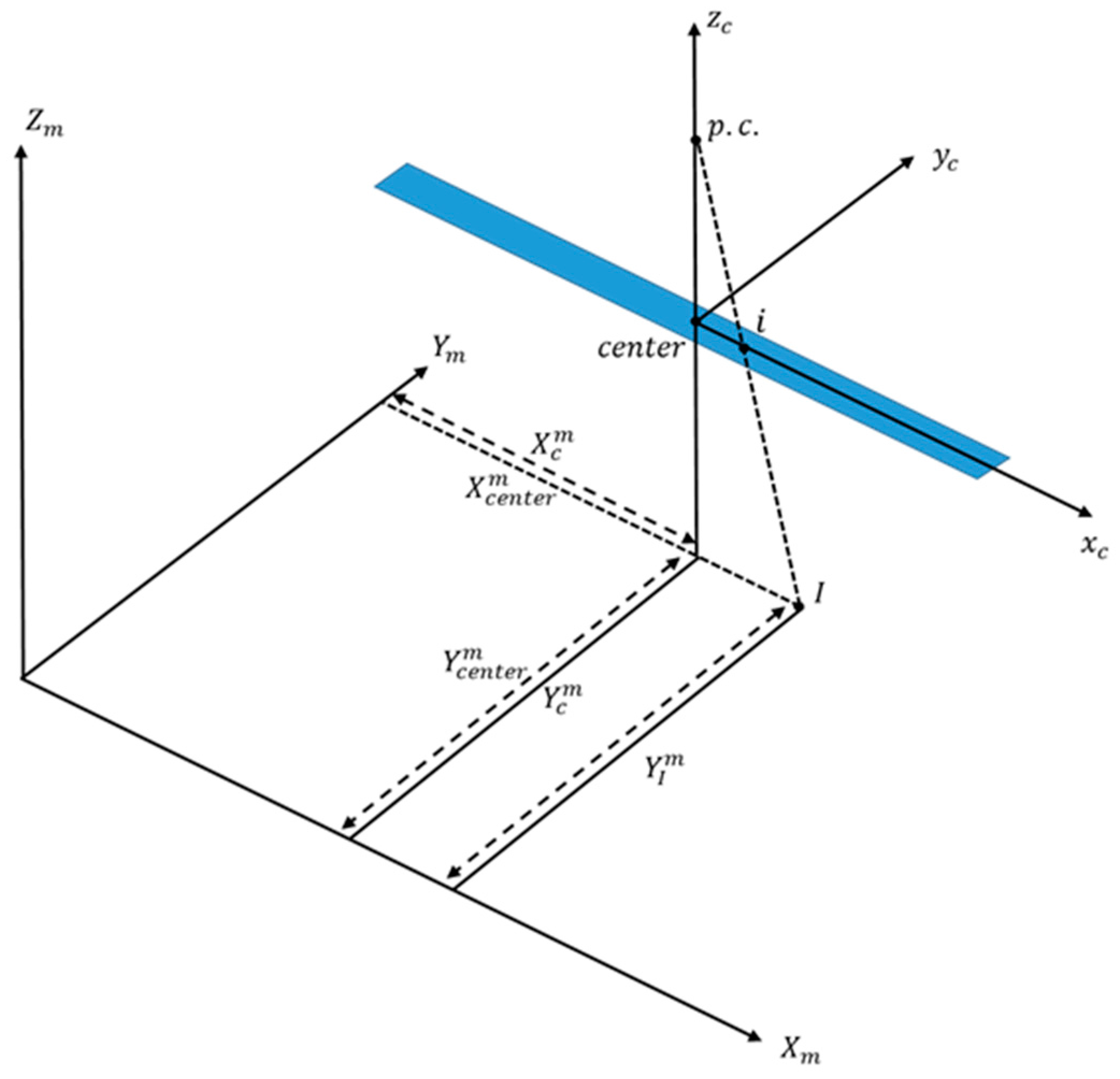
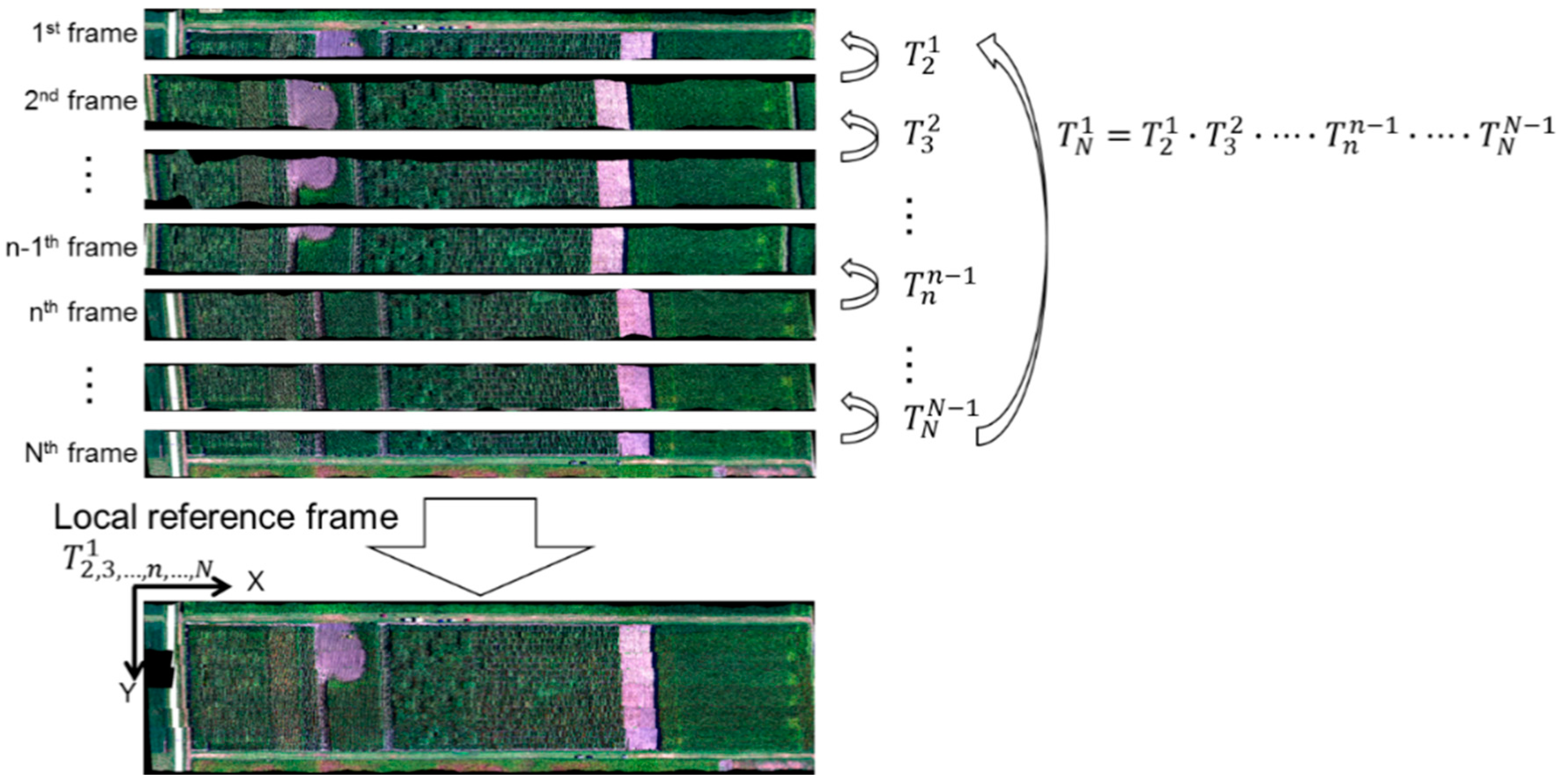
2.3.1. Approximate Evaluation of the Geometric Transformation Relating Partially-Rectified Hyperspectral Orthophotos

To facilitate the identification of tie points among the partially-rectified hyperspectral and RGB-based orthophotos, we first derive an approximate geometric transformation that describes the relative alignment between neighboring hyperspectral orthophotos. As mentioned earlier, the consumer-grade characteristic of the utilized GNSS/INS unit leads to misalignment among the partially-rectified hyperspectral orthophotos. To this end, tie points between adjacent partially-rectified hyperspectral orthophotos are extracted and used to derive a set of transformation parameters that better describe the relative alignment of their reference frames. In this research, the modified SURF-based matching approach is used to detect tie points while considering the impact of GNSS/INS-based direct geo-referencing on the geometric quality of the partially-rectified hyperspectral orthophotos. Having derived a set of tie points between neighboring partially-rectified hyperspectral orthophotos, the parameters of an approximate transformation function that relates the reference frames of those orthophotos could be derived. Since we only seek to derive an approximate geometric transformation, a global affine transformation, which considers possible shifts, rotation, shear and scale variation, is used. Assuming that we have N partially-rectified hyperspectral orthophotos collected from different flight lines (similar to those in Figure 6), one can sequentially evaluate the parameters of the global affine transformation relating successive hyperspectral orthophotos. Tie points between the orthophotos from the first and second flight lines are identified and used to estimate the parameters of the affine transformation $T_2^1$ relating the reference frames of these partially-rectified orthophotos. The affine transformation parameters between the resulting orthophotos from the remaining flight lines (i.e., $T_3^2$, $T_4^3,\dots ,T_{\mathrm{n}}^{\mathrm{n}-1}, \dots ,T_N^{N-1}$, where $T_{\mathrm{n}}^{\mathrm{n}-1}$ denotes the affine transformation relating the reference frames of the n-th and (n − 1)-th orthophotos) can be estimated in a similar manner. Just for visual illustration of the impact of such alignment, the established transformation functions can be used to resample the different orthophotos to the reference frame of the first partially-rectified hyperspectral orthophoto. For example, the n-th partially-rectified hyperspectral orthophoto can be transformed to the reference frame of the first partially-rectified hyperspectral orthophoto through a sequence of transformation multiplications (i.e., $T_n^1=T_2^1·T_3^2·\dots ·T_n^{n-1}$). Figure 6 represents the conceptual basis of how to transform the partially-rectified hyperspectral orthophotos to the reference frame of the first one. Error propagation is expected through this sequential transformation. However, this is not a critical issue since this procedure only aims to derive an approximate geometric transformation between neighboring partially-rectified hyperspectral orthophotos. These transformation functions are then used to constrain the spatial search space when matching the partially-rectified hyperspectral and RGB-based orthophotos.

Even though the tie points are extracted while using the modified SURF approach, they might still include a few mismatched points (outliers). To reduce their impact, we apply the Least Median Square (LMedS) approach to determine the parameters of the global affine transformation relating the reference frames of two neighboring partially-rectified hyperspectral orthophotos [35].

2.3.2. Spatial-Search Space Constrained Identification of Tie Points among the RGB-Based and Partially-Rectified Hyperspectral Orthophotos

The derived geometric relationship between neighboring partially-rectified hyperspectral orthophotos can be used to constrain the spatial search space for the identification of tie points among the RGB-based and partially-rectified hyperspectral orthophotos. The identification of tie points between the partially-rectified hyperspectral and RGB-based orthophotos proceeds sequentially from the first hyperspectral flight line. Throughout this sequential procedure, the identified tie points are used to derive an approximate geometric transformation between the hyperspectral flight line in question and the RGB-based orthophoto. This transformation function is then used, together with the derived transformation functions in the previous section, to produce a refined transformation function for the next hyperspectral flight line.

The spatial extent of the search space for tie points between the RGB-based orthophoto and the first partially-rectified hyperspectral orthophoto is initially based on the quality of the GNSS/INS-based direct geo-referencing information. For example, in this research, the geometric accuracies of the RGB-based and partially-rectified hyperspectral orthophotos are approximately $\pm$0.04 m and $\pm$5 m, respectively. Therefore, the radius of the spatial search space is set to 6 m. The identified tie points within the RGB-based and the first partially-rectified hyperspectral orthophotos are then used to derive an initial transformation function, which is based on a global affine transformation, $T_1^{RGB}\left(initial\right)$. The locations of detected features in the first partially-rectified hyperspectral orthophoto are transformed to the reference frame of the RGB-based orthophoto using $T_1^{RGB}\left(initial\right)$, which is used to define a reduced spatial search space to identify a new set of matched features. Those tie features are then used to derive a refined set of the parameters defining the approximate transformation between the first partially-rectified and RGB-based orthophotos, $T_1^{RGB}\left(refined\right)$. Then, the search space for the second hyperspectral flight line is evaluated while using a derived transformation function, $T_2^{RGB}\left(initial\right)=T_1^{RGB}\left(refined\right)T_2^1$, where $T_2^1$ is the estimated transformation function relating the first and second partially-rectified hyperspectral orthophotos. $T_2^{RGB}\left(initial\right)$ is used to define a constrained search space for the identification of corresponding features between the second partially-rectified hyperspectral and the RGB-based orthophotos. These tie points are then used to derive a refined transformation function relating the second partially-rectified hyperspectral and the RGB-based orthophotos, $T_2^{RGB}\left(refined\right)$. This process is repeated for the subsequent partially-rectified hyperspectral orthophotos to identify tie points and refine the approximate transformation functions relating the partially-rectified hyperspectral and RGB-based orthophotos. A generalized form for the initial transformation function relating the partially-rectified hyperspectral orthophoto from the n-th flight line and the RGB-based orthophoto is derived according to Equation (2).

$$T_n^{RGB}\left(initial\right)=T_{n-1}^{RGB}\left(refined\right)·T_n^{n-1}$$

(2)

where $T_n^{n-1}$ denotes the established transformation function relating the reference frames of the partially-rectified hyperspectral orthophotos from the (n − 1)-th and n-th flight lines. It should be noted that such a transformation function is only used to constrain the spatial domain search space for the identification of conjugate tie points. The extracted tie points among the partially-rectified hyperspectral and RGB-based orthophotos are finally used to derive a more accurate transformation function, as explained in the next section.

2.4. Registration of the RGB and Partially-Rectified Hyperspectral Orthophotos

The transformation function relating the partially-rectified hyperspectral and RGB-based orthophotos is based on the proposed methodology in [5]. Following is a brief theoretical background for such a transformation function. The derivation is based on the assumption that the hyperspectral data are captured by a nadir-looking push-broom scanner mounted on a UAV to acquire data perpendicular to the flight direction. The point positioning equation for a push-broom scanner operating in such a manner is illustrated by the vector summation in Equation (3).

$$r_I^m=r_c^m+{\lambda }_i{R}_c^m{r}_i^c$$

(3)

where $r_I^m$ denotes the vector comprised of the object coordinates of point $I$ relative to the mapping reference frame; $r_i^c$ denotes the coordinates of the corresponding image point $i$ relative to the scanner coordinate system; $r_c^m$ denotes the position of the scanner perspective center relative to the mapping reference frame; $R_c^m$ is the rotation matrix describing the attitude of the scanner coordinate system relative to the mapping reference frame; and ${\lambda }_i$ is the scale factor associated with image point $i$. The position and orientation ($r_c^m, R_c^m$) of a push-broom scanner are time-dependent, i.e., these parameters change from one scan line to the next.

The GNSS/INS direct geo-referencing unit provides an estimate for $r_c^m$ and $R_c^m$ at the epoch when the object point $I$ has been imaged. A consumer-grade GNSS/INS unit is expected to have residual errors $\delta r_c^m$ and $\delta R_c^m$ in the scanner position and orientation information, which will lead to biased object coordinates $r_I^m\left(biased\right)$ for point $I$, as shown in Equation (4). The scaling error $\delta {\lambda }_i$ in Equation (4) represents the cumulative impact of the erroneous scanner position and orientation on the scale factor ${\lambda }_i$. Equation (4) can be expanded to the form in Equation (5). As can be derived from Equation (3), ${\lambda }_i{R}_c^m{r}_i^c$ is equivalent to $r_I^m-r_c^m$. Therefore, Equation (5) can be simplified to the form in Equation (6) after ignoring second order residual errors in the product $\delta {\lambda }_i\delta R_c^m$ (i.e., $\delta {\lambda }_i\delta R_c^m\approx \delta {\lambda }_i{I}_3$, where $I_3$ is a 3 × 3 identity matrix).

$$r_I^m\left(biased\right)=r_c^m+\delta r_c^m+\left({\lambda }_i+\delta {\lambda }_i\right)\delta R_c^m{R}_c^m{r}_i^c$$

(4)

where $\mathsf{\delta }{R}_c^m=\left[\begin{array}{ccc}1& -\mathsf{\Delta }\kappa & \mathsf{\Delta }\phi \\ \mathsf{\Delta }\kappa & 1& -\mathsf{\Delta }\omega \\ -\mathsf{\Delta }\phi & \mathsf{\Delta }\omega & 1\end{array}\right]$ with $\mathsf{\Delta }\omega ,\mathsf{\Delta }\phi ,\mathsf{\Delta }\kappa$ representing the residual errors in the scanner orientation information:

$$r_I^m\left(biased\right)=r_c^m+\delta r_c^m+{\lambda }_i\delta R_c^m{R}_c^m{r}_i^c+\delta {\lambda }_i\delta R_c^m{R}_c^m{r}_i^c$$

(5)

$$r_I^m\left(biased\right)=r_c^m+\delta r_c^m+(\delta R_c^m+\frac{\delta {\lambda }_i}{{\lambda }_i}{I}_3)\left(r_I^m-r_c^m\right)$$

(6)

$$r_I^m\left(biased\right)=r_c^m+\delta r_c^m+\left[\begin{array}{ccc}\frac{\delta {\lambda }_i}{{\lambda }_i}+1& -\mathsf{\Delta }\kappa & \mathsf{\Delta }\phi \\ \mathsf{\Delta }\kappa & \frac{\delta {\lambda }_i}{{\lambda }_i}+1& -\mathsf{\Delta }\omega \\ -\mathsf{\Delta }\phi & \mathsf{\Delta }\omega & \frac{\delta {\lambda }_i}{{\lambda }_i}+1\end{array}\right]\left[\begin{array}{c}{X}_I^m-X_c^m\\ Y_I^m-Y_c^m\\ Z_I^m-Z_c^m\end{array}\right]$$

(7)

Equation (7) represents the impact of residual errors in the direct geo-referencing information on the ground coordinates of object points. For the center of the scanner that encompasses the image point $i$, the corresponding biased coordinates $r_{center}^m\left(biased\right)$ can be derived from Equation (6) to produce the form in Equation (8). For a nadir-looking vertical scanner (refer to Figure 7), $r_{center}^m-r_c^m$ will be equivalent to ${\left(0,0,-h\right)}^T$, where $h$ is the flying height above ground. Accordingly, Equation (8) reduces to the form in Equation (9), which could be reformulated to the form in Equation (10), where one can see that $X_c^m=X_{center}^m\left(biased\right)-\delta X_c^m+h\mathsf{\Delta }\phi$.

$$r_{center}^m\left(biased\right)=r_c^m+\delta r_c^m+(\delta R_c^m+\frac{\delta {\lambda }_c}{{\lambda }_c}{I}_3)\left(r_{center}^m-r_c^m\right)$$

(8)

where $r_{center}^m-r_c^m$ is equivalent to $\left[\begin{array}{c}{X}_{center}^m-X_c^m\\ Y_{center}^m-Y_c^m\\ Z_{center}^m-Z_c^m\end{array}\right]$:

$$r_{center}^m\left(biased\right)=r_c^m+\delta r_c^m+(\delta R_c^m+\frac{\delta {\lambda }_c}{{\lambda }_c}{I}_3)\left[\begin{array}{c}0\\ 0\\ -h\end{array}\right]$$

(9)

$$\left[\begin{array}{c}{X}_{center}^m\left(biased\right)\\ Y_{center}^m\left(biased\right)\\ Z_{center}^m\left(biased\right)\end{array}\right]=\left[\begin{array}{c}{X}_c^m\\ Y_c^m\\ Z_c^m\end{array}\right]+\left[\begin{array}{c}\delta X_c^m\\ \delta Y_c^m\\ \delta Z_c^m\end{array}\right]+\left[\begin{array}{c}-h\Delta \phi \\ h\mathsf{\Delta }\omega \\ -h(\frac{\delta {\lambda }_c}{{\lambda }_c}+1)\end{array}\right]$$

(10)

Equation (7) can be simplified to the form in Equation (11) while considering a nadir-looking vertical scanner, i.e., $Y_I^m\approx Y_c^m$, over a relatively flat object space, i.e., $Z_I^m-Z_c^m=-h$ (refer to Figure 7). For a partially-rectified hyperspectral orthophoto, we are only dealing with the planimetric coordinates. Therefore, we are only concerned with the $xy$-coordinates in Equation (11). Since it has been already established that $X_c^m=X_{center}^m\left(biased\right)-\delta X_c^m+h\mathsf{\Delta }\phi$, the $xy$-coordinates in Equation (11) can be rewritten as shown in Equation (12), and after ignoring higher-order residual terms, the latter would reduce to the form in Equation (13).

$$r_I^m\left(biased\right)=r_c^m+\delta r_c^m+\left[\begin{array}{ccc}\frac{\delta {\lambda }_i}{{\lambda }_i}+1& -\mathsf{\Delta }\kappa & \mathsf{\Delta }\phi \\ \mathsf{\Delta }\kappa & \frac{\delta {\lambda }_i}{{\lambda }_i}+1& -\mathsf{\Delta }\omega \\ -\mathsf{\Delta }\phi & \mathsf{\Delta }\omega & \frac{\delta {\lambda }_i}{{\lambda }_i}+1\end{array}\right]\left[\begin{array}{c}{X}_I^m-X_c^m\\ 0\\ -h\end{array}\right]$$

(11)

$$\left[\begin{array}{c}{X}_I^m\left(biased\right)\\ Y_I^m\left(biased\right)\end{array}\right]=\left[\begin{array}{c}{X}_c^m\\ Y_c^m\end{array}\right]+\left[\begin{array}{c}\delta X_c^m\\ \delta Y_c^m\end{array}\right]+\left[\begin{array}{c}-h\mathsf{\Delta }\phi \\ h\mathsf{\Delta }\omega \end{array}\right]+\left[\begin{array}{c}\frac{\delta {\lambda }_i}{{\lambda }_i}+1\\ \mathsf{\Delta }\kappa \end{array}\right]\left(X_I^m-X_c^m\right)$$

(12)

$$\left[\begin{array}{c}{X}_I^m\left(biased\right)\\ Y_I^m\left(biased\right)\end{array}\right]=\left[\begin{array}{c}{X}_{center}^m\left(biased\right)-\delta X_c^m+h\mathsf{\Delta }\phi \\ Y_I^m\end{array}\right]+\left[\begin{array}{c}\delta X_c^m-h\mathsf{\Delta }\phi \\ \delta Y_c^m+h\mathsf{\Delta }\omega \end{array}\right]+\left[\begin{array}{c}\frac{\delta {\lambda }_i}{{\lambda }_i}+1\\ \mathsf{\Delta }\kappa \end{array}\right]\left(X_I^m-X_{center}^m\left(biased\right)\right)+\left[\begin{array}{c}\frac{\delta {\lambda }_i}{{\lambda }_i}+1\\ \mathsf{\Delta }\kappa \end{array}\right]\left(\delta X_c^m-h\mathsf{\Delta }\phi \right)$$

(13)

$$\left[\begin{array}{c}{X}_I^m\left(biased\right)-X_{center}^m\left(biased\right)\\ Y_I^m\left(biased\right)-Y_I^m\end{array}\right]=\left[\begin{array}{c}\delta X_c^m-h\mathsf{\Delta }\phi \\ \delta Y_c^m+h\mathsf{\Delta }\omega \end{array}\right]+\left[\begin{array}{c}\frac{\delta {\lambda }_i}{{\lambda }_i}+1\\ \mathsf{\Delta }\kappa \end{array}\right]\left(X_I^m-X_{center}^m\left(biased\right)\right)$$

(14)

Equation (14) represents the transformation function relating the biased planimetric coordinates $\left(X_I^m\left(biased\right), Y_I^m\left(biased\right)\right)$ and true coordinates $\left(X_I^m, Y_I^m\right)$ of an object point $I$ in terms of the residual errors in the direct geo-referencing information $\left(\delta X_c^m,\delta Y_c^m,\mathsf{\Delta }\omega ,\mathsf{\Delta }\phi ,\mathsf{\Delta }\kappa \mathrm{and}\delta {\lambda }_i\right)$. For the problem at hand, $\left(X_I^m\left(biased\right), Y_I^m\left(biased\right)\right)$ correspond to the observed coordinates in the partially-rectified hyperspectral orthophoto, which will be denoted as $\left(X_{hyper-o},Y_{hyper-o}\right)$, while $\left(X_I^m, Y_I^m\right)$ correspond to the true coordinates as represented in the RGB-based orthophoto, which will be denoted as $\left(X_{RGB-o},Y_{RGB-o}\right)$. Therefore, the final transformation function $T_{RGB}^{Hyperspectral}$ can be represented by Equation (15). Since the residual errors in the direct geo-referencing information change along the system trajectory, they are time dependent, so Equation (15) is re-parameterized to the form in Equation (16). Thus, the registration between the partially-rectified hyperspectral and the RGB-based orthophotos requires estimation of the parameters $\left[a_0\left(t\right),b_0\left(t\right),a_1\left(t\right),b_1\left(t\right)\right]$. It should be noted that $Y_{hyper-o}$ can be used to represent the time of exposures for the different scan lines. Since it is reasonable to assume that residual errors in the GNSS/INS position and orientation information gradually change throughout the hyperspectral flight line, we use the concept of reference points where we only solve for the transformation function parameters at their locations. The transformation parameters at any epoch can be then derived through an interpolation function that depends on the transformation parameters associated with the reference points. More details regarding the resampling of the partially-rectified hyperspectral orthophotos to match the reference frame of the RGB-based orthophoto can be found in [5].

$$\left[\begin{array}{c}{X}_{hyper-o}-X_{hyper-o\left(center\right)}\\ Y_{hyper-o}-Y_{RGB-o}\end{array}\right]=\left[\begin{array}{c}\delta X_c^m-h\mathsf{\Delta }\phi \\ \delta Y_c^m+h\mathsf{\Delta }\omega \end{array}\right]+\left[\begin{array}{c}\frac{\delta {\lambda }_i}{{\lambda }_i}+1\\ \mathsf{\Delta }\kappa \end{array}\right]\left(X_{RGB-o}-X_{hyper-o\left(center\right)}\right)$$

(15)

$$\left[\begin{array}{c}{X}_{hyper-o}\left(t\right)-X_{hyper-o\left(center\right)}\left(t\right)\\ Y_{hyper-o}\left(t\right)-Y_{RGB-o}\end{array}\right]=\left[\begin{array}{c}{a}_0\left(t\right)\\ b_0\left(t\right)\end{array}\right]+\left[\begin{array}{c}{a}_1\left(t\right)\\ b_1\left(t\right)\end{array}\right]\left[X_{RGB-o}-X_{hyper-o\left(center\right)}\left(t\right)\right]$$

(16)

$$\mathrm{where} \{\begin{array}{l}{a}_0\left(t\right)=\delta X_c^m\left(t\right)-h\mathsf{\Delta }\phi \left(t\right)\hfill \\ b_0\left(t\right)=\delta Y_c^m\left(t\right)+h\mathsf{\Delta }\omega \left(t\right)\hfill \\ a_1\left(t\right)=\frac{\delta {\lambda }_i\left(t\right)}{{\lambda }_i\left(t\right)}+1\hfill \\ b_1\left(t\right)=\mathsf{\Delta }\kappa \left(t\right)\hfill \end{array}$$

3. Experimental Results

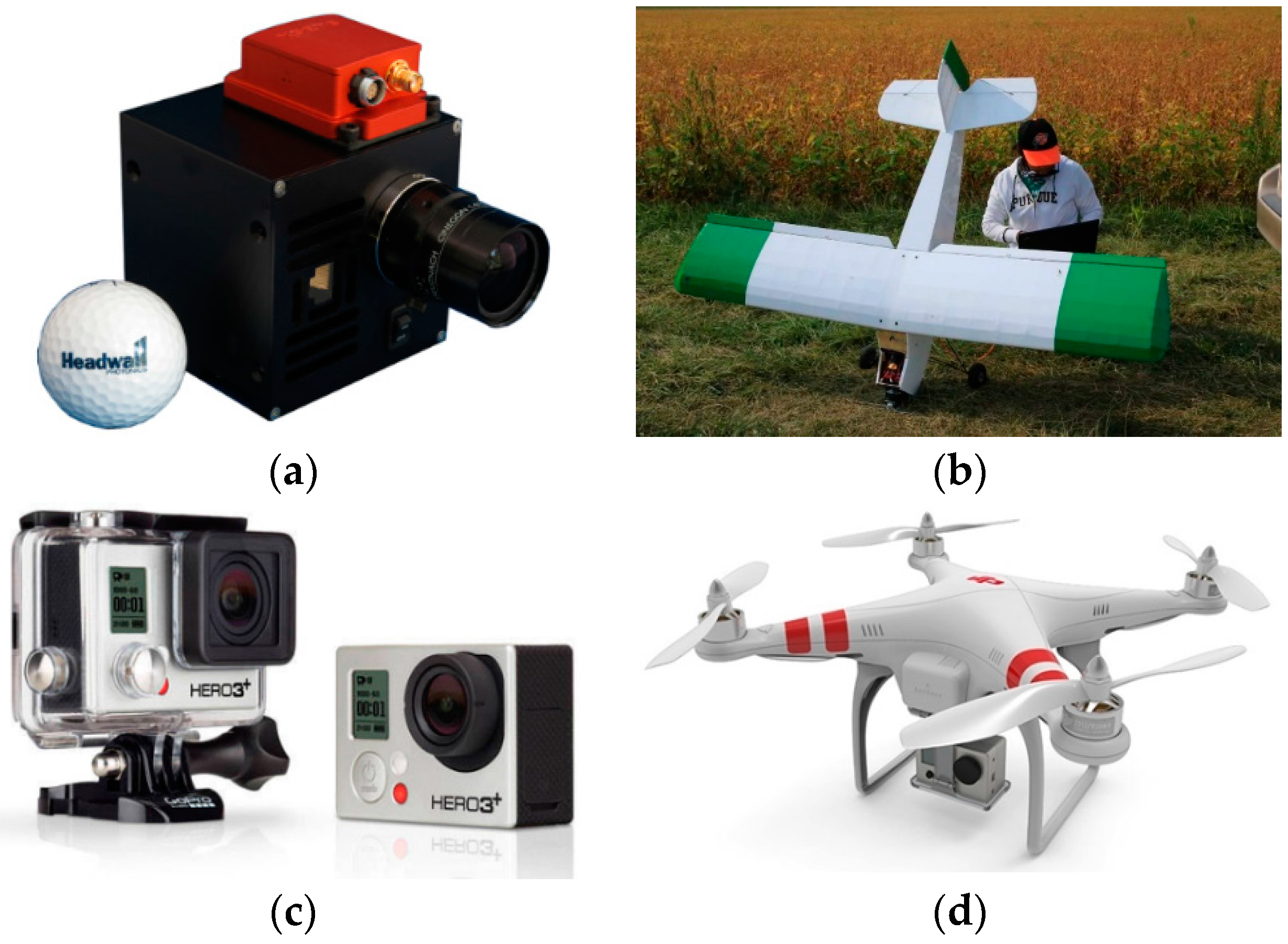
3.1. Test Site and Dataset Description

This section outlines the test site and data characteristics to confirm the effectiveness of the proposed approach in automatically improving the geometric quality of partially-rectified hyperspectral orthophotos. The agricultural test field, which is comprised of plots planted with multiple varieties of sorghum, is located within the Agronomy Center for Research and Education (ACRE) at Purdue University, Lafayette, IN, USA. The test field dimensions are approximately 100 m (along the north-south direction) by 250 m (along the east-west direction). The plant rows are aligned along the north-south direction with alleys separating the ranges between the plots along the east-west direction. The datasets are comprised of hyperspectral and RGB scenes, which are captured by a push-broom scanner (Figure 8a) mounted on a fixed-wing UAV platform (Figure 8b) and an RGB frame camera (Figure 8c) mounted on a quadcopter (Figure 8d), respectively. Specifications of the utilized RGB and hyperspectral sensors are illustrated in

Table 1. Specifications of RGB and hyperspectral imaging sensors

	RGB Frame Camera	Hyperspectral Push-Broom Scanner
Acquisition date	25 July 2015	4 August 2015
		21 August 2015
Focal length	3 mm	17 mm
Spatial resolution	1.5 cm (frame image)	5 cm (partially-rectified orthophoto)
	4 cm (generated orthophoto)
Geometric accuracy (orthophoto)	±0.04 m	±5 m
Spectral resolution	3 bands (RGB)	278 bands with a 2.2-nm width for each band

.

For the acquisition of RGB images, a GoPro Hero 3+ digital frame camera, which is easier to handle and capable of providing stable high resolution images from a consumer-grade UAV platform, is used. The GoPro camera, whose the lens has a 3-mm nominal focal length, was calibrated using the USGS Simultaneous Multi-frame Analytical Calibration (SMAC) distortion model [36]. A DJI Phantom 2 quadcopter, which is equipped with the GoPro camera mounted on a gimbal to ensure that images are acquired with the camera’s optical axis pointing in the nadir direction, was flown over the test field on 25 July 2015. It was flown along 11 flight lines at a data rate of two frames/s from a flying height of roughly 15 m with the platform moving at a speed of 8 m/s and the camera operating at the medium field-of-view mode. The forward overlap and side lap are 60%. During the total flight time of about 25 min, 540 RGB images are captured over the sorghum field. This flight configuration resulted in a 1.5-cm GSD. The RGB-based orthophoto was generated from the acquired frame images through the following procedure. The whole process for the orthophoto generation used in-house developed software coded in C++.

• A Structure from Motion (SfM) approach [37] is applied to derive the Exterior Orientation Parameters (EOPs) for the captured images and a sparse point cloud representing the field relative to an arbitrarily-defined reference frame.
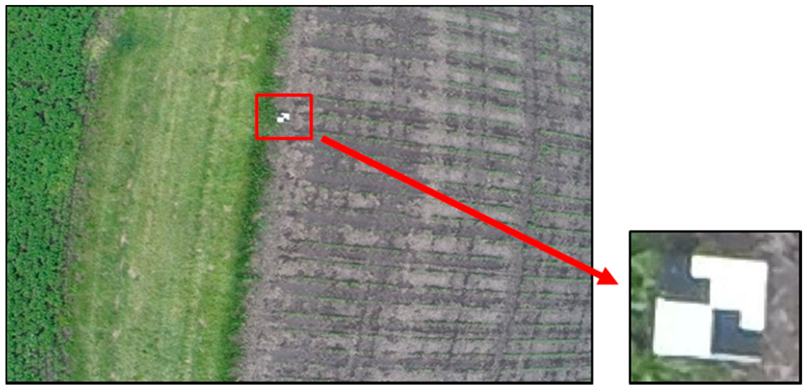
• An absolute orientation process is then applied to transform the derived point cloud and estimated EOPs to a global mapping reference frame. Signalized GCPs, whose coordinates are derived through an RTK GPS survey (10 GCPs are measured), are used to estimate the absolute orientation parameters for the SfM-based point cloud and EOPs (refer to Figure 9 for a close-up image of one of the targets). Then, a global bundle adjustment is carried out to refine the EOPs of the different images and sparse point-cloud coordinates relative to the GCPs’ reference frame.
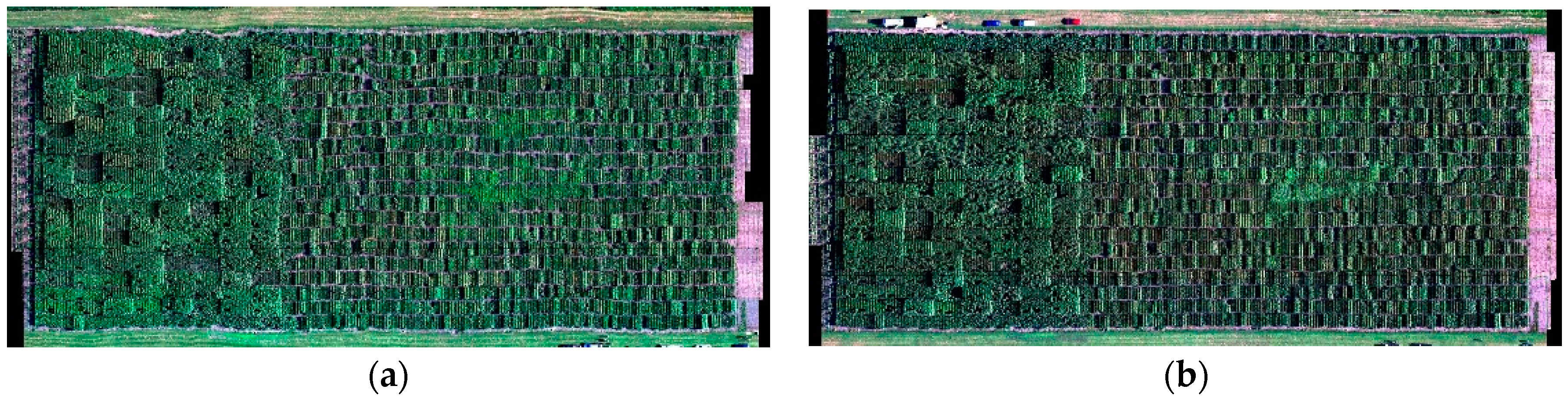
• A DEM is interpolated from the sparse point cloud. The bundle-based EOPs and the camera IOPs, as well as the DEM are finally used to produce an RGB-based orthophoto mosaic of the entire test field (Figure 10). One should note that the color variation between the north and south portions in the orthophoto is caused by illumination differences between the data acquisition epochs. The RGB-based orthophoto has a 4-cm GSD with the Root Mean Square Error (RMSE) of the X, Y and Z coordinates for 20 check points being 2 cm, 3 cm and 6 cm, respectively.

The hyperspectral data were acquired by a Headwall Nano-Hyperspec push-broom scanner. It has 278 spectral bands of approximately 2.2 nm in width over the range of 400–1000 nm. It acquires 640 pixels along the scan line and was operated at a scan rate of 330 lines/s with a lens that has a 17-mm nominal focal length. For these experiments, the Nano-Hyperspec was equipped with an Xsense MTi-G-700 navigation unit having a gyro bias stability of 10$°$/h (orange box in Figure 8a). The hyperspectral data were collected from the fixed-wing UAV while flying at a speed of approximately 16 m/s from an altitude of roughly 120 m. The corresponding GSD for such a flight configuration was roughly 5 cm. Software provided by Headwall was employed to generate the partially-rectified hyperspectral orthophoto with the help of the generated DEM from the frame imagery. According to the Xsense’s specifications, the geometric accuracy of the partially-rectified orthophotos is in the range of $\pm$5 m.

Two hyperspectral datasets, each consisting of seven flight lines with 50% side lap, are acquired on different dates (4 August 2015 and 21 August 2015). Figure 11 shows the mosaicked partially-rectified hyperspectral orthophoto from the captured data on 21 August 2015. A closer visual inspection of this orthophoto reveals geometric misalignments between neighboring partially-rectified hyperspectral orthophotos. Figure 11 also shows a heading error, which is manifested in non-orthogonality between the plant rows and alleys between the plots, as well as misalignment of the plant rows in neighboring partially-rectified hyperspectral orthophotos.

3.2. Results and Analysis

To illustrate the effectiveness of the proposed approach for improving the geometric quality of the partially-rectified hyperspectral orthophoto, we implemented the modified SURF for the automated extraction of tie points among the RGB and hyperspectral orthophotos. Three bands in the RGB portion of the spectrum can be used for the identification of tie points. The red band generally showed stable results for detecting tie points due to the enhanced contrast related to green vegetation and was selected to detect tie points. The proposed procedure is based on some thresholds, which are set according to the properties of the scenes and sensor characteristics. Specifically, the scale threshold for accepting detected features as matching candidates, $T_{\sigma }$, was set to five (this scale corresponds to an approximately 36 $\times$ 36 pixel window in the input images as per [22]). The radius of the spatial search space varied according to the nature of the involved images within the different stages of the proposed procedure. For the orthophotos where we relied on the GNSS/INS information as the only source for constraining the spatial search space (i.e., identification of tie points between neighboring partially-rectified hyperspectral orthophotos and between the RGB-based orthophoto and the first partially-rectified hyperspectral orthophoto), the radius was set to 6 m, which is based on the expected performance of the Xsense MTi-G-700 navigation unit. For tie point identification between the partially-rectified hyperspectral and RGB-based orthophotos while considering the approximate affine transformation function, the spatial search radius was set to 3 m. The scale ratio threshold, $T_S$, for determining the scale-domain search space was set to 0.8. The ratio threshold for the closest and second closest Euclidean distance between the descriptors for the potential matching candidates in the template and query images, $T_r$, was set to 0.8, as suggested in [21]. The number of reference points for the interpolation of the transformation function relating the RGB-based and partially-rectified hyperspectral orthophotos was set to four, as proposed in [5]. The experiments are implemented in MATLAB using a computer with 16 GB RAM and Intel(R) Core(TM) i7-6700 CPU @3.40 GHz. The execution time of the whole process to generate the refined 3-band orthophoto in this environment is around 3 min.

The number of extracted tie points between neighboring partially-rectified hyperspectral orthophotos for the different dates is presented in

Table 2. Number of identified tie point pairs between neighboring partially-rectified hyperspectral orthophotos.

Flight Lines	Number of Extracted Tie Point Pairs
	4 August 2015	21 August 2015
Pass 1–2	203	126
Pass 2–3	303	350
Pass 3–4	202	269
Pass 4–5	89	210
Pass 5–6	306	341
Pass 6–7	295	351

, where one can see that a sufficient number of tie points was detected. These tie points were used to evaluate the parameters of the approximate transformation function relating the partially-rectified hyperspectral orthophotos ($T_n^{n-1}$), which was then used to evaluate the approximate transformation function between the RGB-based and partially-rectified hyperspectral orthophotos ($T_n^{RGB}\left(initial/refined\right)$).

Refined hyperspectral orthophotos for both datasets are illustrated in Figure 12, which shows the derived mosaic from the seven flight lines. This figure shows good alignment of the plant rows among the different flight lines. Qualitative evaluation of the improvement in the geometric fidelity of the partially-rectified hyperspectral orthophotos can be established by visually inspecting the alignment between plant rows and alleys between plots following their resampling to the reference frame of the RGB-based orthophoto. For illustrative comparison, some subareas of the partially-rectified and refined hyperspectral orthophotos are presented in Figure 13. As indicated in Figure 13a, the non-orthogonality between the plant rows and alleys separating the ranges in the partially-rectified hyperspectral orthophoto is quite obvious. The corresponding areas in Figure 13b illustrate that orthogonality between the plant rows and ranges has been successfully recovered. A further qualitative evaluation is presented in Figure 14, which shows a chessboard orthophoto mosaic from the RGB-based and refined hyperspectral orthophotos. Figure 12, Figure 13 and Figure 14 clearly illustrate the capability of the proposed procedure to automatically identify tie points and successfully evaluate the appropriate transformation function that models the impact of residual errors in the GNSS/INS-based navigation information.

For quantitative evaluation of the refined hyperspectral orthophotos, the following measures were employed: (1) the quality of fit between the automatically-extracted tie points used for the estimation of the parameters of the transformation function, before and after improving the hyperspectral orthophotos; (2) the quality of fit between the manually-extracted tie point and linear features while using the derived transformation parameters from the automatically-extracted and manually-identified tie features. The quality of fit is based on the RMSE of the spatial separation between conjugate features before and after refining the geometric quality of the RGB bands of the hyperspectral orthophotos.

Table 3. Accuracy assessment of the quality of fit between the RGB-based and hyperspectral data before and after the geometric refinement for the acquired hyperspectral data on 4 August 2015.

	RMSE for the Automatically-Extracted Features Using the Estimated Transformation Parameters from the Proposed Procedure			RMSE for the Manually-Extracted Features Using the Estimated Transformation Parameters from the Manual and Proposed Procedures
	Number of Features	RMSE (Before) (m)	RMSE (After) (m)	Number of Features	Transformation Parameters from Manual Measurements (m)	Transformation Parameters from Automatically-Extracted Features (m)
Pass 1	25 points	4.54	0.69	14 points and 25 lines	0.26	0.84
Pass 2	122 points	5.09	0.67	27 lines	0.29	0.67
Pass 3	95 points	4.57	0.46	14 points and 22 lines	0.21	0.36
Pass 4	94 points	4.27	0.63	26 lines	0.33	0.72
Pass 5	173 points	3.54	0.35	14 points and 33 lines	0.31	0.63
Pass 6	68 points	5.00	0.99	24 lines	0.28	0.96
Pass 7	178 points	2.75	0.55	28 lines	0.29	0.49

and

Table 4. Accuracy assessment of the quality of fit between the RGB-based and hyperspectral data before and after the geometric refinement for the acquired hyperspectral data on 21 August 2015.

	RMSE for the Automatically-Extracted Features Using the Estimated Transformation Parameters from the Proposed Procedure			RMSE for the Manually-Extracted Features Using the Estimated Transformation Parameters from the Manual and Proposed Procedures
	Number of Features	RMSE (Before) (m)	RMSE (After) (m)	Number of Features	Transformation Parameters from Manual Measurements (m)	Transformation Parameters from Automatically-Extracted Features (m)
Pass 1	26 points	3.15	0.70	14 points and 25 lines	0.19	0.78
Pass 2	86 points	4.51	0.66	26 lines	0.19	0.78
Pass 3	64 points	2.08	0.51	14 points and 26 lines	0.19	0.37
Pass4	64 points	3.70	0.70	27 lines	0.18	0.77
Pass 5	117 points	1.80	0.58	26 lines	0.15	0.35
Pass 6	58 points	4.15	0.72	26 lines	0.22	0.70
Pass 7	101 points	1.42	0.62	26 lines	0.20	0.38

present the derived statistics of the quality of fit for the RGB bands of the two hyperspectral datasets. A closer inspection of the results in these tables reveals the following:

• Although the quality of fit for the manually-based transformation parameters is better than the automatically-based ones, the proposed approach is capable of improving the quality of partially-rectified hyperspectral orthophotos without the need for manual intervention. The proposed automated approach has improved the quality of fit from roughly 5 m to almost 0.6 m. In this regard, one should note that the utilized quality of fit is biased towards the manually-based transformation parameters, since the right half of Table 3 and Table 4 is based on the manually-identified features both for the estimation of the transformation parameters and evaluating the quality of fit.
• The proposed approach tends to show better performance when the original direct geo-referencing information is relatively accurate. In other words, whenever the quality of fit before the refinement is relatively high (i.e., small RMSE value), the corresponding quality of fit after the refinement is significantly improved.
• The number of automatically-identified tie points does not have a significant impact on the quality of the hyperspectral orthophoto refinement. It can be seen from the accuracy assessment of the quality of fit that the RMSE among the tie points using the estimated transformation parameters showed similar values regardless of the number of identified tie points.

4. Conclusions and Recommendations for Future Work

Low-cost UAVs equipped with RGB and hyperspectral imaging systems are promising remote sensing platforms for high throughput phenotyping. However, the payload restriction and limited endurance of those platforms impose the use of consumer-grade direct geo-referencing units with moderate ability to determine the position and orientation of the associated sensors. For frame cameras, recent advances in system calibration and triangulation procedures allow for the generation of RGB-based orthophotos with high geometric fidelity using consumer-grade navigation data and/or limited GCPs. For hyperspectral push-broom scanners, the derived geospatial data are quite sensitive to the quality of the direct geo-referencing information. The integration of frame and push-broom scanner imagery can help to mitigate the negative impact of the geo-referencing information while improving the geometric quality of the rectified hyperspectral orthophotos.

The paper presented an automated approach for improving the ortho-rectification of hyperspectral push-broom scanner imagery using RGB-based frame imagery. More specifically, an RGB-based orthophoto is used to improve the geometric quality of a partially-rectified hyperspectral orthophoto contaminated by the impact of residual errors in the direct geo-referencing information. The paper proposed an approach that automatically detects tie points between the RGB-based and partially-rectified hyperspectral orthophotos through a modified SURF procedure that can be used when dealing with agricultural scenes exhibiting repetitive patterns of rows. The modified SURF increases the reliability of the matching procedure by imposing constraints on the scale for the detected features, the main orientation of such features, as well as the spatial extent of the search space. The spatial extent of the search space is reduced through a two-step procedure that starts with using an approximate geometric transformation to improve the alignment between neighboring partially-rectified hyperspectral orthophotos. Then, these geometric transformation functions are used to restrict the search space for the identification of tie points in the partially-rectified hyperspectral and RGB-based orthophotos. The identified tie features are finally used to estimate the parameters of a more appropriate transformation function relating the RGB and hyperspectral orthophotos in the presence of residual errors in the GNSS/INS geo-referencing information. Experimental results from real datasets have qualitatively and quantitatively demonstrated the feasibility of the proposed methodology in improving the quality of fit between the RGB-based and refined hyperspectral orthophotos by one order of magnitude from 5.0 m to almost 0.6 m.

To further improve the geometric quality of hyperspectral data, future work will focus on improved identification of tie points between the original hyperspectral and frame scenes. Moreover, automated identification of linear conjugate features, as well as tie points will be investigated. These tie features will be used in a global bundle adjustment together with the GNSS/INS navigation data to improve the geo-referencing quality of the whole dataset.

References

1. Candiago, S.; Remondino, F.; De Giglio, M.; Dubbini, M.; Gattelli, M. Evaluating Multispectral Images and Vegetation Indices for Precision Farming Applications from UAV Images. Remote Sens. 2015, 7, 4026–4047. [Google Scholar] [CrossRef]
2. Fiorani, F.; Schurr, U. Future scenarios for plant phenotyping. Annu. Rev. Plant Biol. 2013, 64, 267–291. [Google Scholar] [CrossRef] [PubMed]
3. Busemeyer, L.; Mentrup, D.; Möller, K.; Wunder, E.; Alheit, K.; Hahn, V.; Maurer, H.P.; Reif, J.C.; Würschum, T.; Müller, J.; et al. BreedVision—A Multi-Sensor Platform for Non-Destructive Field-Based Phenotyping in Plant Breeding. Sensors 2013, 13, 2830–2847. [Google Scholar] [CrossRef] [PubMed]
4. Tao, V.; Li, J. Advances in Mobile Mapping Technology; ISPRS Book Series No. 4; Taylor & Francis: London, UK, 2007. [Google Scholar]
5. Habib, A.; Xiong, W.; He, F.; Yang, H.; Crawford, M. Improving Orthorectification of UAV-based Push-broom Scanner Imagery using Derived Orthophotos from Frame Cameras. IEEE J. Sel. Top. Appl. Earth Obs. Remote Sens. 2016. [Google Scholar] [CrossRef]
6. Zhang, C.; Kovacs, J.M. The Application of Small Unmanned Aerial Systems for Precision Agriculture: A Review. Precis. Agric. 2012, 13, 693–712. [Google Scholar] [CrossRef]
7. Honkavaara, E.; Saari, H.; Kaivosoja, J.; Pölönen, I.; Hakala, T.; Litkey, P.; Mäkynen, J.; Pesonen, L. Processing and Assessment of Spectrometric, Stereoscopic Imagery Collected using a Lightweight UAV Spectral Camera for Precision Agriculture. Remote Sens. 2013, 5, 5006–5039. [Google Scholar] [CrossRef] [Green Version]
8. Hernandez, A.; Murcia, H.; Copot, C.; De Keyser, R. Towards the Development of a Smart Flying Sensor: Illustration in the Field of Precision Agriculture. Sensors 2015, 15, 16688–16709. [Google Scholar] [CrossRef] [PubMed] [Green Version]
9. Araus, J.L.; Cairns, J.E. Field High-throughput Phenotyping: The New Crop Breeding Frontier. Trends Plant Sci. 2014, 19, 52–61. [Google Scholar] [CrossRef] [PubMed]
10. Aasen, H.; Burkart, A.; Bolten, A.; Bareth, G. Generating 3D Hyperspectral Information with Lightweight UAV Snapshot Cameras for Vegetation Monitoring: From Camera Calibration to Quality Assurance. ISPRS J. Photogramm. Remote Sens. 2015, 108, 245–259. [Google Scholar] [CrossRef]
11. Burkart, A.; Aasen, H.; Alonso, L.; Menz, G.; Bareth, G.; Rascher, U. Angular Dependency of Hyperspectral Measurements over Wheat Characterized by a Novel UAV based Goniometer. Remote Sens. 2015, 7, 725–746. [Google Scholar] [CrossRef]
12. Deery, D.; Jimenez-Berni, J.; Jones, H.; Sirault, X.; Furbank, R. Proximal Remote Sensing Buggies and Potential Applications for Field based Phenotyping. Agronomy 2014, 4, 349–379. [Google Scholar] [CrossRef]
13. Lawrence, K.C.; Park, B.; Windham, W.R.; Mao, C. Calibration of a Pushbroom Hyperspectral Imaging System for Agricultural Inspection. Trans. Am. Soc. Agric. Eng. 2003, 46, 513–522. [Google Scholar] [CrossRef]
14. Inoue, Y.; Sakaiya, E.; Zhu, Y.; Takahashi, W. Diagnostic Mapping of Canopy Nitrogen Content in Rice based on Hyperspectral Measurements. Remote Sens. Environ. 2012, 126, 210–221. [Google Scholar] [CrossRef]
15. Mitchell, J.J.; Glenn, N.F.; Sankey, T.T.; Derryberry, D.R.; Germino, M.J. Remote Sensing of Sagebrush Canopy Nitrogen. Remote Sens. Environ. 2012, 124, 217–223. [Google Scholar] [CrossRef]
16. Berni, J.A.; Zarco-Tejada, P.J.; Suárez, L.; Fereres, E. Thermal and Narrowband Multispectral Remote Sensing for Vegetation Monitoring from an Unmanned Aerial Vehicle. IEEE Trans. Geosci. Remote Sens. 2009, 47, 722–738. [Google Scholar] [CrossRef]
17. Habib, A.F.; Morgan, M.; Lee, Y. Bundle Adjustment with Self-Calibration using Straight Lines. Photogramm. Rec. 2002, 17, 635–650. [Google Scholar] [CrossRef]
18. Remondino, F.; Barazzetti, L.; Nex, F.; Scaioni, M.; Sarazzi, D. UAV Photogrammetry for Mapping and 3D Modeling—Current Status and Future Perspectives. Int. Arch. Photogramm. Remote Sens. Spat. Inf. Sci. 2011, 38, 25–31. [Google Scholar] [CrossRef]
19. Suomalainen, J.; Anders, N.; Iqbal, S.; Roerink, G.; Franke, J.; Wenting, P.; Hünniger, D.; Bartholomeus, H.; Becker, R.; Kooistra, L. A Lightweight Hyperspectral Mapping System and Photogrammetric Processing Chain for Unmanned Aerial Vehicles. Remote Sens. 2014, 6, 11013–11030. [Google Scholar] [CrossRef]
20. Ramirez-Paredes, J.-P.; Lary, D.J.; Gans, N.R. Low-altitude Terrestrial Spectroscopy from a Pushbroom Sensor. J. Field Robot. 2016, 33, 837–852. [Google Scholar] [CrossRef]
21. Lowe, D.G. Distinctive image features from Scale-invariant Keypoints. Int. J. Comput. Vis. 2004, 60, 91–110. [Google Scholar] [CrossRef]
22. Bay, H.; Ess, A.; Tuytelaars, T.; Gool, L.V. SURF Speeded Up Robust Features. Comput. Vis. Image Underst. 2008, 110, 346–359. [Google Scholar] [CrossRef]
23. Harris, C.; Stephens, M. A Combined Corner and Edge Detector. In Proceedings of the Alvey Vision Conference, Manchester, UK, 31 August–2 September 1988; pp. 147–152.
24. Sedaghat, A.; Mokhtarzade, M.; Ebadi, H. Uniform Robust Scale-invariant Feature Matching for Optical Remote Sensing Images. IEEE Trans. Geosci. Remote Sens. 2011, 49, 4516–4527. [Google Scholar] [CrossRef]
25. Han, Y.; Choi, J.; Byun, Y.; Kim, Y. Parameter Optimization for the Extraction of Matching Points between High-resolution Multisensor Images in Urban Areas. IEEE Trans. Geosci. Remote Sens. 2014, 52, 5612–5621. [Google Scholar]
26. Huo, C.; Pan, C.; Huo, L.; Zhou, Z. Multilevel SIFT Matching for Large-size VHR Image Registration. IEEE Geosci. Remote Sens. Lett. 2012, 9, 171–175. [Google Scholar] [CrossRef]
27. Wang, L.; Niu, Z.; Wu, C.; Xiie, R.; Huang, H. A Robust Multisource Image Automatic Registration System based on the SIFT Descriptor. Int. J. Remote Sens. 2012, 33, 3850–3869. [Google Scholar] [CrossRef]
28. Yu, L.; Zhang, D.; Holden, E.J. A Fast and Fully Automatic Registration Approach based on Point Features for Multi-source Remote-sensing Images. Comput. Geosci. 2008, 34, 838–848. [Google Scholar] [CrossRef]
29. Fan, B.; Huo, C.; Pan, C.; Kong, Q. Registration of Optical and SAR Satellite Images by Exploring the Spatial Relationship of the Improved SIFT. IEEE Geosci. Remote Sens. Lett. 2013, 10, 657–661. [Google Scholar] [CrossRef]
30. Han, Y.; Byun, Y.; Choi, J.; Han, D.; Kim, Y. Automatic Registration of High-resolution Images using Local Properties of Features. Photogramm. Eng. Remote Sens. 2012, 78, 211–221. [Google Scholar] [CrossRef]
31. Kang, Z.Z.; Jia, F.M.; Zhang, L.Q. A Robust Image Matching Method based on Optimized BaySAC. Photogramm. Eng. Remote Sens. 2012, 80, 1041–1052. [Google Scholar] [CrossRef]
32. Han, Y.; Byun, Y. Automatic and Accurate Registration of VHR Optical and SAR Images using a Quadtree Structure. Int. J. Remote Sens. 2015, 36, 2277–2295. [Google Scholar] [CrossRef]
33. Long, T.; Jiao, W.; He, G.; Zhang, Z.A. Fast and Reliable Matching Method for Automated Georeferencing of Remotely-Sensed Imagery. Remote Sens. 2016, 8, 56. [Google Scholar] [CrossRef]
34. Liu, F.; Bi, F.; Chen, L.; Shi, H.; Liu, W. Feature-area Optimization: A Novel SAR Image Registration Method. IEEE Geosci. Remote Sens. Lett. 2016, 13, 242–246. [Google Scholar] [CrossRef]
35. Meer, P.; Mintz, D.; Rosenfeld, A. Robust Regression Methods for Computer Vision: A Review. Int. J. Comput. Vis. 1991, 6, 59–70. [Google Scholar] [CrossRef]
36. He, F.; Habib, A. Target-based and Feature-based Calibration of Low-cost Digital Cameras with Large Field-of-view. In Proceedings of the ASPRS Annual Conference, Tampa, FL, USA, 4–8 April 2015.
37. He, F.; Habib, A. Linear Approach for Initial Recovery of the Exterior Orientation Parameters of Randomly Captured Images by Low-cost Mobile Mapping System. Int. Arch. Photogramm. Remote Sens. Spat. Inf. Sci. 2014, 1, 149–154. [Google Scholar] [CrossRef]
Figure 1. Flowchart of the proposed methodology for the automated registration of RGB-based and partially-rectified hyperspectral orthophotos.
Remotesensing 08 00796 g001
Figure 2. Portion of a partially-rectified hyperspectral orthophoto that shows a repetitive pattern within an agricultural field (RGB bands are displayed).
Remotesensing 08 00796 g002
Figure 3. Extracted features over an agricultural field at different scales: (a) fine-scale features; and (b) coarse-scale features.
Remotesensing 08 00796 g003
Figure 4. Search space constraints in the spatial and scale domains. The radius and the height of the cylinder represent the extent of the search space in the spatial and scale domains, respectively, for a feature in the template image (i.e., marked white circle).
Remotesensing 08 00796 g004
Figure 5. Comparison of the matching performance for acquired imagery over an agricultural field: (a) SURF and (b) modified SURF strategies.
Remotesensing 08 00796 g005
Figure 6. Conceptual basis of the implemented procedure for describing the geometric transformations between neighboring partially-rectified hyperspectral orthophotos.
Remotesensing 08 00796 g006
Figure 7. Imaging geometry of a nadir-looking vertical push-broom hyperspectral scanner.
Remotesensing 08 00796 g007
Figure 8. Sensors and UAVs utilized for dataset acquisition: (a) hyperspectral push-broom scanner mounted on (b) a fixed-wing UAV and (c) RGB frame camera mounted on (d) a quad copter UAV.
Remotesensing 08 00796 g008
Figure 9. Sample RGB image over the test field with a close-up of one of the targets.
Remotesensing 08 00796 g009
Figure 10. RGB-based orthophoto of the test field derived from the captured frame images on 25 July 2015.
Remotesensing 08 00796 g010
Figure 11. Mosaicked partially-rectified orthophoto of hyperspectral data over the test field captured on 21 August 2015 (only the RGB bands are displayed) showing heading errors and misalignment between neighboring flight lines.
Remotesensing 08 00796 g011
Figure 12. Mosaicked refined hyperspectral orthophoto through the proposed approach: (a) acquired data on 4 August 2015 and (b) acquired data on 21 August 2015.
Remotesensing 08 00796 g012
Figure 13. Subareas of the test field for visual inspection of the registration result: (a) partially-rectified hyperspectral orthophoto and (b) refined hyperspectral orthophoto generated by the proposed approach.
Remotesensing 08 00796 g013aRemotesensing 08 00796 g013b
Figure 14. Close-up of chessboard orthophoto mosaics generated from the RGB-based orthophoto and refined hyperspectral orthophoto through the proposed approach: (a) acquired hyperspectral data on 4 August 2015 and (b) acquired hyperspectral data on 21 August 2015.
Remotesensing 08 00796 g014