A Physically Constrained Calibration Database for Land Surface Temperature Using Infrared Retrieval Algorithms

Abstract

Land surface temperature (LST) is routinely retrieved from remote sensing instruments using semi-empirical relationships between top of atmosphere (TOA) radiances and LST, using ancillary data such as total column water vapor or emissivity. These algorithms are calibrated using a set of forward radiative transfer simulations that return the TOA radiances given the LST and the thermodynamic profiles. The simulations are done in order to cover a wide range of surface and atmospheric conditions and viewing geometries. This study analyzes calibration strategies while considering some of the most critical factors that need to be taken into account when building a calibration dataset, covering the full dynamic range of relevant variables. A sensitivity analysis of split-windows and single channel algorithms revealed that selecting a set of atmospheric profiles that spans the full range of surface temperatures and total column water vapor combinations that are physically possible seems beneficial for the quality of the regression model. However, the calibration is extremely sensitive to the low-level structure of the atmosphere, indicating that the presence of atmospheric boundary layer features such as temperature inversions or strong vertical gradients of thermodynamic properties may affect LST retrievals in a non-trivial way. This article describes the criteria established in the EUMETSAT Land Surface Analysis—Satellite Application Facility to calibrate its LST algorithms, applied both for current and forthcoming sensors.

1. Introduction

Land surface temperature (LST) is an important parameter in the physics of the Earth’s surface. LST controls the surface-emitted long-wave radiation and is thereby essential to quantify sensible and latent heat fluxes between the Earth’s surface and the atmosphere. These interactions are crucial for a variety of applications related to land surface processes, such as climate and drought monitoring [1,2], hydrological cycle [3,4,5], model assessment [6,7,8,9], and data assimilation [10,11,12], among others. LST has been retrieved in remote sensing platforms using a variety of algorithms that rely on sensor channels in the so-called atmospheric window region of the infrared spectrum [13]. Within this band, surface-emitted radiances reach the sensor with relatively little absorption by the atmosphere. Moreover, in the thermal infrared atmospheric window (TIR), surface emissivity can be determined with relatively less uncertainty than in other regions in the infrared, such as in the middle infrared, making it ideal to retrieve surface properties [14]. Previous studies proposed the use of channels in the middle infrared for LST estimation [13,15,16]; however, these are far less common than algorithms based on the thermal infrared observations and therefore will not be considered here.

The choice of LST algorithm, which is often a semi-empirical function of top-of-atmosphere (TOA) brightness temperatures in TIR, is intrinsically linked to the characteristics of the sensor being used. As such, LST algorithms may rely on a single channel (the mono-window algorithms, MW), when measurements are available in only one TIR band [15,17,18,19], or in a combination of TIR channels using the so-called generalized split-windows (GSW) approach [13,20,21]. In general, this type of algorithm is based on a linear regression between the measured quantities at the top of the atmosphere and LST, using ancillary data such as spectral emissivity, total column water vapor (TCWV), zenith viewing angle (ZVA), land cover and also day/night flags. Usually these parameters are divided into classes, and for each combination a set of model coefficients is estimated [13,20]. The whole procedure therefore requires setting up a comprehensive calibration database which is usually generated ad hoc, with a high risk of leaving out unforeseen situations that lead to systematic biases in operational retrievals. To the best of our knowledge, no study has been devoted to the process of building a calibration database. This paper focuses on the factors that need to be taken into account when building a calibration database for such regressions, providing a general methodology that can be applied when developing an algorithm for infrared LST estimates and providing a systematic discussion of the impact of all the choices that are made when building a calibration database.

In order to make the model coefficients robust enough to deal with any combination of input parameters, it is necessary to calibrate the model for a wide range of atmospheric and surface conditions as well as viewing geometries. A good calibration of the model coefficients can only be achieved if the calibration database is designed carefully, covering the range of variations that are expected to affect the problem [21]. Usually, the models are calibrated using criteria that are considered reasonable, covering a wide range of atmospheric and surface conditions [20,22], but here we propose an objective approach to prepare a calibration database that minimizes the overall model error statistics and their variations among the range of input parameters.

This article summarizes the procedure used in the EUMETSAT LSA SAF [23] to calibrate LST algorithms for the Spinning Enhanced Visible and InfraRed Imager (SEVIRI, e.g., [20]) onboard the Meteosat Second Generation (MSG), the Advanced Very-High Resolution Radiometer (AVHRR) on Metop and the Meteosat Visible and InfraRed Imager (MVIRI) onboard Meteosat First Generation (MFG; e.g., [17]). The current standard methodology within the LSA SAF uses a criterion for setting up the calibration database with a good compromise, addressing the widest possible retrieval conditions (which are a pre-requisite for a global LST product), but a sensitivity analysis was required to ensure that the most robust possible model coefficients are in use. A similar exercise will be soon performed for the Flexible Combined Imager (FCI) on board the Meteosat Third Generation (MTG; [24]) to design the follow-on of LSA SAF operational LST products.

2. Methodology

2.1. The Problem

Considering the Earth surface as a lambertian emitter-reflector, a cloud-free atmosphere under local thermodynamic equilibrium and negligible atmospheric scattering, the monochromatic top of atmosphere radiance $L_i$, in a given channel i, and measured by a sensor onboard a satellite observing the Earth’s surface under zenith angle θ is expressed by (e.g., [13]):

$$L_i\left(\mathsf{\theta }\right)=B\left(T_{bi}\right)={ϵ}_i{B}_i\left(T_{sfc}\right){\tau }_i\left(\theta \right)+L_{atm,i}^{\uparrow }\left(\theta \right)+\left(1-{ϵ}_i\right)L_{atm,i}^{\downarrow }{\tau }_i\left(\theta \right)$$

(1)

where ${ϵ}_i$ is the surface emissivity on channel i, $B_i\left(T_{sfc}\right)$ is the equivalent black-body radiance at temperature $T_{sfc}$ (or LST), ${\tau }_i$ is the transmissivity, $L_{atm,i}^{\uparrow }$ is the upward atmosphere-emitted radiance, and $L_{atm,i}^{\downarrow }$ is the downward atmosphere-emitted radiance. LST is often estimated from linearized inversions of Equation (1), applied to one or more channels in the TIR, as mentioned above. There are a few formulations of these inversions in the literature [25] which mostly depend on how the Taylor expansion of the radiative transfer equation is made in order to derive a formulation that is suitable to a particular application. In this work, the sensitivity to the used model is not fully addressed, although some of the results could be slightly different if different LST algorithms were used. However, it is important to assess the differences of using a GSW model or a MW model, as they serve two different purposes: the first is widely used in state-of-the-art retrieval schemes in sensors with two or more channels in the thermal atmospheric window, while the second is left for sensors with only one channel in that band. Here, only one formulation for each case is considered—one GSW and one MW algorithm—which will serve as testbeds for the calibration datasets under analysis. The GSW formulation used for operational LST estimates both from the Moderate Resolution Imaging Spectroradiometer (MODIS; [21]) and from SEVIRI ([20]):

$$LST=C+\left(A_1+A_2\frac{1-ϵ}{ϵ}+A_3\frac{\mathrm{\Delta }ϵ}{{ϵ}^2}\right)\frac{T_{IR1}+T_{IR2}}{2}+\left(B_1+B_2\frac{1-ϵ}{ϵ}+B_3\frac{\mathrm{\Delta }ϵ}{{ϵ}^2}\right)\frac{T_{IR1}-T_{IR2}}{2}$$

(2)

where $A_1,A_2,A_3,B_1,B_2,B_3$ and $C$ are the model coefficients, $T_{IR1}$ and $T_{IR2}$ are the equivalent brightness temperatures, $ϵ$ and $\mathrm{\Delta }ϵ$ are the average and the difference of the emissivities in both split-windows channels. For the MW model, the formulation derived by Duguay-Tetzlaff et al. [17] to derive LST from Meteosat First Generation is used:

$$LST=A\frac{T_{IR1}}{{ϵ}_{IR1}}+B\frac{1}{{ϵ}_{IR1}}+C,$$

(3)

where $A$, $B$, and $C$ are again the regression coefficients. In both cases, the regression coefficients are fit for classes of TCWV and ZVA, and they must somehow simulate atmospheric absorption and emission, while the effect of surface emissivity is in these cases, explicitly resolved. The atmospheric transmissivity is mainly constrained by the radiative optical path. Hence, a good calibration database to fit model coefficients in Equations (2) and (3) needs to ensure that a scene may be observed by a wide range of viewing geometries (ZVA) and water vapor contents, which is the most relevant and variable absorber/emitter in the TIR window region.

The weighting functions (given by the vertical derivative of transmissivity) of atmospheric window channels peak close to the surface, where the strongest vertical gradients of humidity are found. However, in the presence of well-developed moist planetary boundary layers, their peak will be higher above (although always relatively close to the ground), which means the temperature and humidity vertical structure at the lower levels in the profiles represented in the calibration database might play a role in the database robustness, especially considering the occurrence of temperature inversions close to the surface. This effect may be taken into account not only by introducing a large variety of atmospheric profiles at different locations and observation times, but also by artificially varying the difference between the surface skin temperature and the near-surface air temperature ($LST-T_{air}$), which in turn has a significant role in the control of the thermal structure of the lower atmosphere, through the turbulent sensible heat flux (e.g., [26,27]). This difference varies across the diurnal cycle, among surface types and for different large scale atmospheric conditions, and may be either positive or negative. Particular attention should be paid to its distribution within calibration databases and to the impact on algorithm performance.

The difference between TOA brightness temperatures in the split-window channels is aimed at capturing differential absorption within those bands which is associated to atmospheric water vapor content. In the case of a GSW algorithm, Equation (3), the difference between the spectral emissivities of the window channels are also taken into account. This difference is related to surface type and moisture in the sense that moister surfaces show less spectral variations in emissivity [28].

2.2. Radiative Transfer Simulations

The development of LST algorithms, such as those represented by Equations (2) and (3) (see e.g., [20,21,25]) is usually based on a set of radiative transfer simulations performed for a calibration database (for algorithm fit) and a validation one (for algorithm test), both representing a wide range of clear sky conditions. The databases must be independent and, while the former should encapsulate the widest possible atmospheric conditions for the area of interest together with broad distributions of surface emissivity and sensor viewing geometry that are needed for robust parameter estimation, the latter should contain the largest possible set of profiles/surface conditions to allow a comprehensive characterization of LST algorithm uncertainty. By LST algorithm uncertainty, we mean deviations of LST retrievals from the “true value” that are not associated to uncertainties in the input data, but solely to the retrieval method. The characterization of the individual sources of uncertainty (such as the algorithm uncertainty studied here or the uncertainty due to emissivity or to the sensor noise, for example) has been recognized as crucial for the uncertainty validation of remotely sensed surface temperature products [29]. It is worth emphasizing that the comparison of LST estimates obtained using actual remote sensing observations against ground-based observations is part of a product validation exercise. In that case, which is often limited to a relatively small number of available sites, the deviations will be the result of both algorithm and input errors and their contributions to the total error are impossible to disentangle. The radiative transfer simulations aim to determine the TOA spectral radiances for each profile in the respective databases, so that the forward problem is solved with full knowledge of the surface emission and atmospheric absorption. It is important that those simulations are performed with an accurate radiative transfer model. For the example analyzed in this study, the MODTRAN4 code [30] was used, which returns spectral radiances with a resolution of 1 cm⁻¹. For the sake of simplicity, MODTRAN4 TOA radiances were convoluted with SEVIRI response functions for channels centered at 10.8 µm (IR1 channel) and 12.0 µm (IR2 channel, only used in the GSW algorithm), and then subject to the inverse Planck function to obtain the respective channels brightness temperatures, $T_{IR1}$ and $T_{IR2}$ (for more details see, e.g., [15]). The calibration of the coefficients is performed using a least-squares technique, aimed to provide the best fit for the semi-empirical relationships between the simulated brightness temperatures and the set of prescribed LSTs, atmospheric conditions and viewing geometries in the calibration database. In the case of Equations (2) and (3) used in this study, the coefficients are calibrated in classes of ZVA and TCWV, as those formulations do not explicitly model their effect on the atmospheric correction. Finally, the algorithm uncertainty is characterized using the independent validation database, through comparisons of estimated LST obtained with one of the semi-empirical models (Equation (2) or (3)) and the $LS{T}_{True}$ value. The latter corresponds to the $T_{Skin}$ values in the databases, which together with the respective atmospheric profiles, surface emissivity and prescribed view zenith angle, led to the TOA brightness temperature(s) used in the LST algorithms. The use of independent databases for algorithm calibration and validation, relying on accurate radiative transfer simulations, is the best way of characterizing the algorithm uncertainty and its performance for a wide range of scenarios.

2.3. Characteristics of Atmospheric Profiles Relevant for Radiative Transfer in the TIR Window

We have opted to select the calibration dataset from a comprehensive collection of clear-sky profiles of temperature, water vapor and ozone, as well as ancillary variables such as spectral emissivity, land cover, elevation, skin temperature, and surface pressure compiled by Borbas et al. [31]. This dataset, hereafter referred to as SeeBor database, includes over 15,000 profiles and will be used in this work for convenience. We could have made use of other datasets also specifically gathered for satellite retrievals under clear sky conditions (e.g., [22]), but our focus is on the criteria to be taken into account for the subset of calibration data for LST algorithms.

Figure 1 shows the geographical distribution of profiles contained in the SeeBor database; the dots representing the profile locations are colored according to their TCWV. This dataset covers the whole globe, including oceans. Regions with more frequent cloud cover are, as expected, somewhat less populated. In general, low values of TCWV are found near the poles and high values close to the Equator. However there are notable exceptions, especially in some continental regions where it is possible to observe both very dry and very moist atmospheres. From this large set of profiles only a few will be selected to calibrate an LST retrieval algorithm, while the rest is used for its validation, i.e., characterization of algorithm uncertainty as mentioned above. The task of selecting these calibration profiles is tricky and impacts the model robustness, as will be shown below.

The statistical distributions of TCWV and skin temperature are shown in Figure 2a,b, respectively. Both distributions are highly skewed. The majority of the profiles are on the drier side of the TCWV distribution and almost no profiles show values of more than 6 cm since those conditions are within the physical limit for an atmosphere with no clouds. Skin temperatures show a wide dynamic range, roughly between 210 and 330 K, the distribution being negatively skewed. Thus, in principle, it would only be necessary to uniformly span these ranges of values to have a comprehensive calibration database. However, some combinations of both parameters are unphysical, which in turn leads to less accurate coefficients and worse performance by the regression model. The bivariate distribution shown in Figure 2c reveals that not surprisingly very moist (clear sky) atmospheres only occur over the warmer surfaces, while towards lower TCWV values, the skin temperature range increases. In other words, the very dry atmospheres can be very warm or very cold, whereas the moister atmospheres are only found over warmer surfaces.

In Figure 3 the distribution of $LST-T_{air}$ is shown, for each class of TCWV. $T_{air}$ corresponds to the temperature at the first pressure level above the ground. The separation in classes of TCWV shows that drier atmospheres support somewhat larger temperature gradients close to the surface. The dynamic range of this parameter needs to be chosen carefully, since it has a large impact on the resulting coefficients (see sensitivity tests in Section 3). Cases with the largest differences should also be accounted for in the linear regression; otherwise, the calibration would miss some of the most extreme low-level temperature profiles and this would degrade the quality of the regression, especially when the algorithm needs to deal with such profiles in practice. For very dry atmospheres, the distribution is nearly normal with maximum absolute differences of about 20 K. In the case of moister atmospheres, the distributions become positively skewed with maximum positive differences of about 25 K for only a few cases but almost no values below −10 K. In general, most cases lie between −15 K and 15 K.

The diversity of land surfaces and the radiative properties of their materials need to be taken into account through an appropriate range of surface emissivities. This quantity adds an extra level of complexity to the calibration database. Depending on the algorithm that is chosen, only one value is used in the case of a single-channel algorithm, or the values on two bands need to be specified in the case of a GSW model. Some GSWs, such as that considered here (Equation (2)) rely on the average value of the emissivity in the two channels and also the difference between them. Therefore it was decided to prescribe a range of emissivity values for the channel around 10.8 µm and then prescribe a range of differences of the emissivities in both channels, $\Delta ϵ={ϵ}_{IR2}-{ϵ}_{IR1}$. The range of spectral emissivities at 10.8 µm and 12.0 µm, close to typical central wavelengths of split-window channels (e.g., MODIS, SEVIRI), available in the SeeBor database are shown in Figure 4. There are quite a few cases with very high emissivities which correspond to SeeBor profiles over water bodies and ice. In general, cases over land have higher emissivities in the 12.0 µm compared to the 10.8 µm. The larger spectral variations are found over deserts and semi-arid surfaces.

The viewing angle also affects the calibration and the appropriate range to be considered will depend on each sensor. In this work the analysis will be for a sensor on board a geostationary platform, or for a large swath polar orbiting sensor, and therefore we will also consider a wide range of view zenith angles.

2.4. A Calibration Database

Given the physical constraints of the problem and the range of the input parameters detailed in the previous section, the following methodology is proposed to select the subset of calibration profiles:

(1)

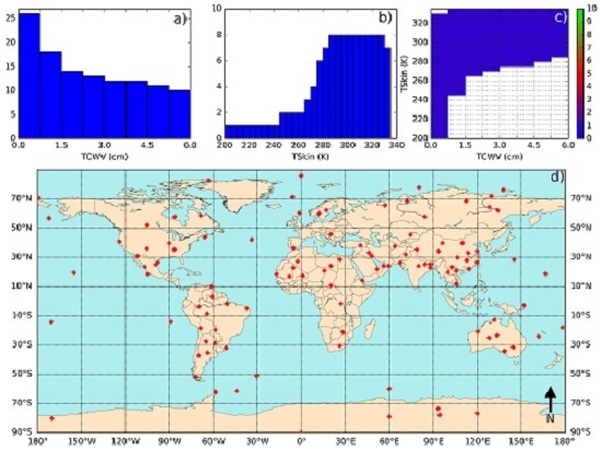
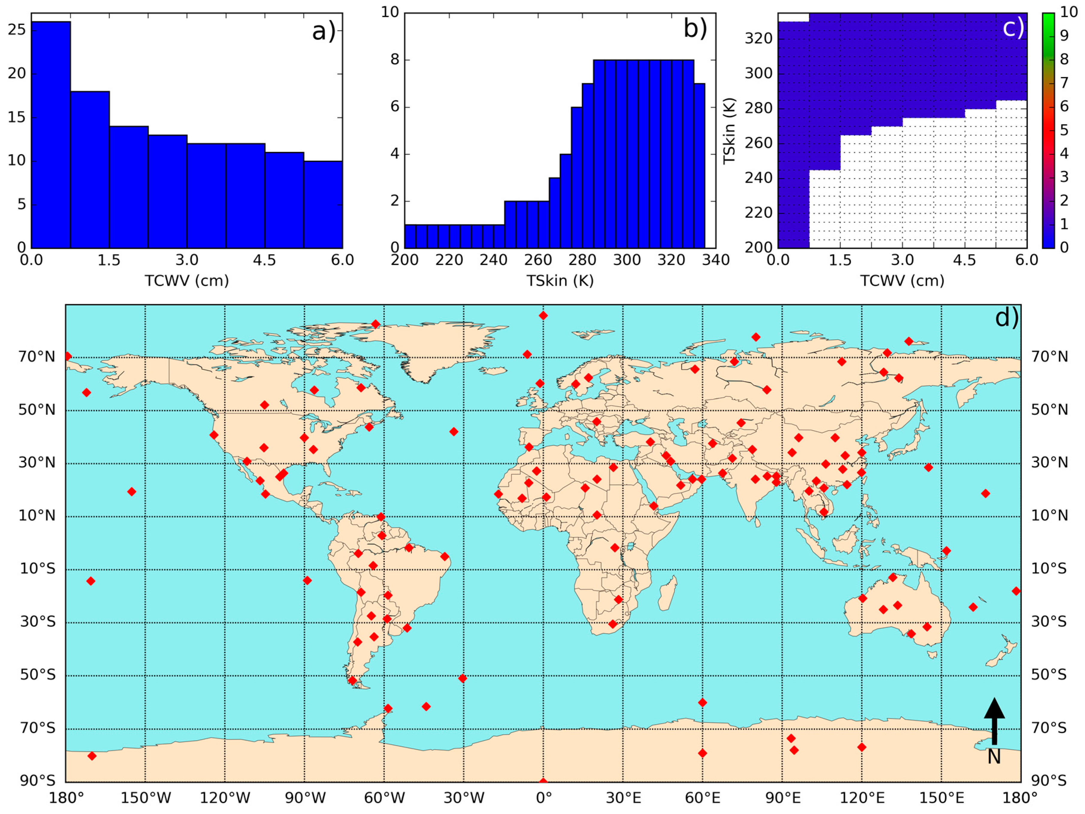
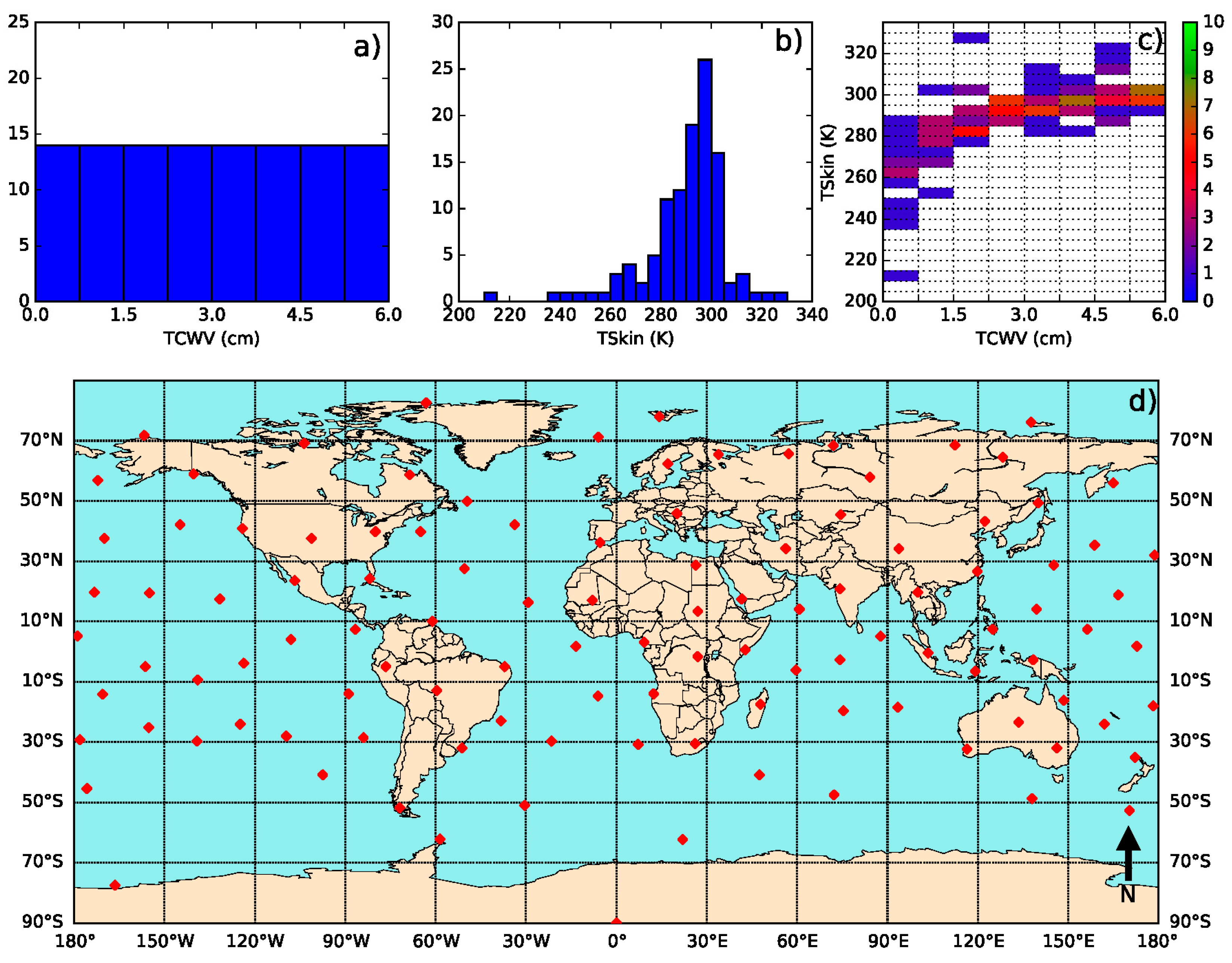
Define classes of $T_{Skin}$ (from 200 K to 330 K in steps of 5 K) and $TCWV$ (from 0 to 6 cm in classes of 0.75 cm—values greater than this should be treated with the coefficient corresponding to the last $TCWV$ class).

(2)

Iterate in the SeeBor clear-sky profile database to fill each class in the $TCWV/T_{Skin}$ phase space (as in Figure 2c) with one case each. When a new profile is selected, it is ensured that its great-circle distance to the already selected profiles is greater than an initial distance of 15 degrees, which guarantees a wide geographical coverage. After a sufficiently large number of tries (in this case 30,000), the distance criterion is relaxed in steps of minus 1 degree, until the whole $TCWV/T_{Skin}$ phase space is filled.

(3)

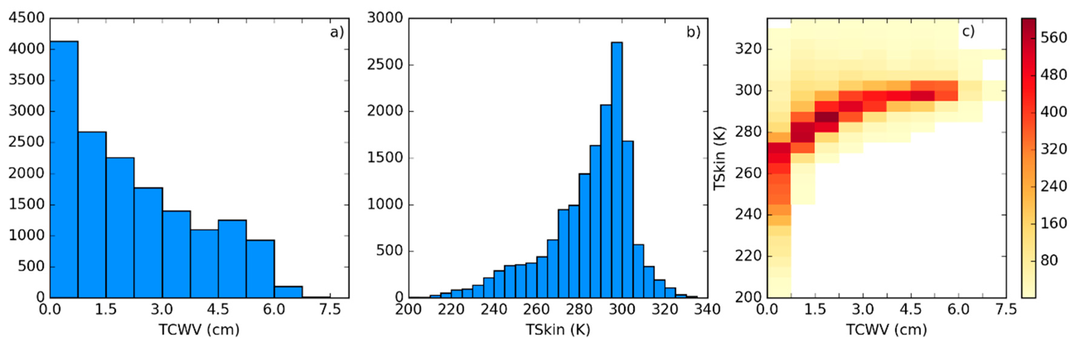
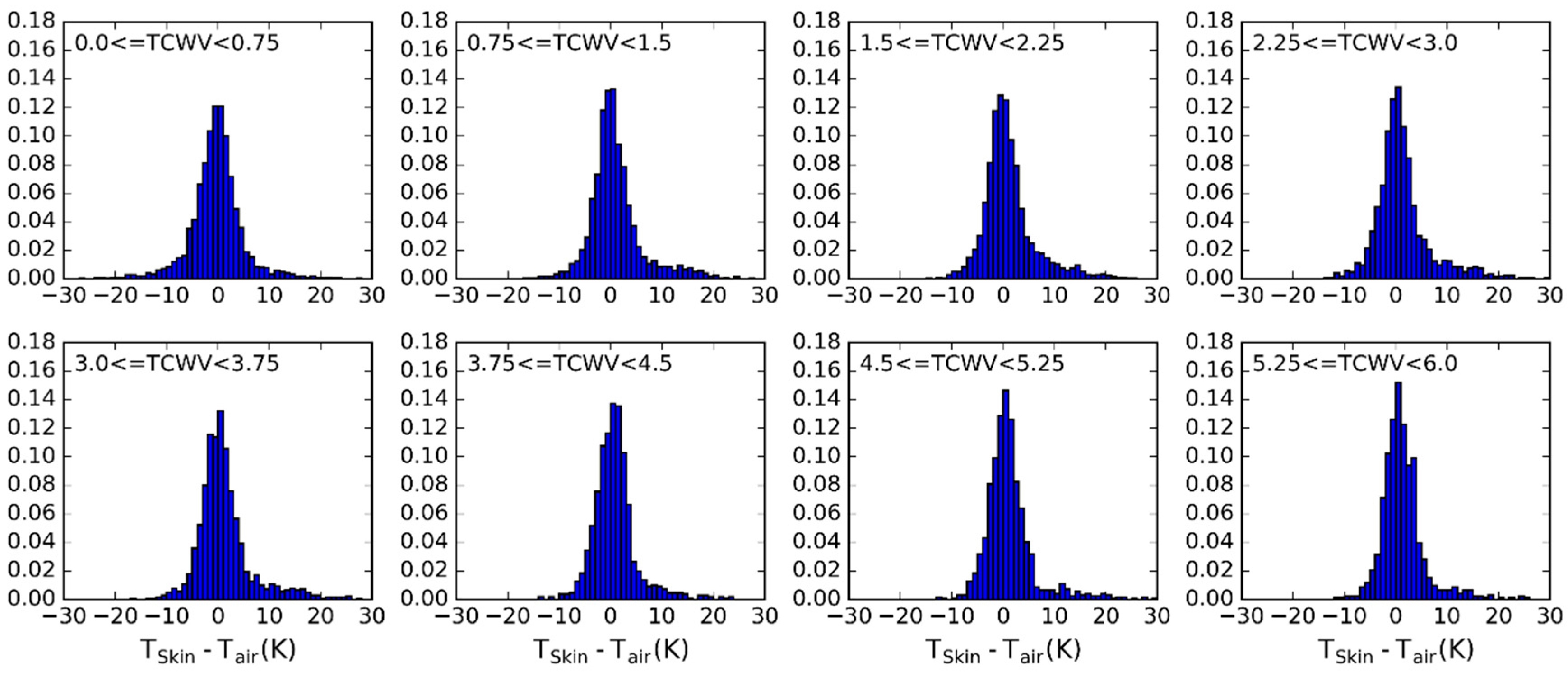
For each of the previously selected profiles, assign a new $T_{Skin}$ based on the ranges of $T_{Skin}-T_{air}$ observed in Figure 3. The choice of the range of perturbations to apply is key to the performance of the chosen model and may depend on the region of interest. In the case of this work, a range of ±15 K around $T_{air}$ in steps of 5 K showed an overall good performance. As will be seen, large biases arise when non-physical cases are included or if the somewhat more extreme cases are not taken into account.

(4)

Each of these conditions may be sensed from angles ranging from 0 (nadir view) to 70° in steps of 2.5°. It is important to discretize the viewing geometry in this way because this is an intrinsically non-linear problem. The upper limit of the $ZVA$ might be adapted for the sensor under analysis. Previous calibration exercises show that above this viewing angle limit the retrieval errors are generally too high, especially for moister atmospheres [15].

(5)

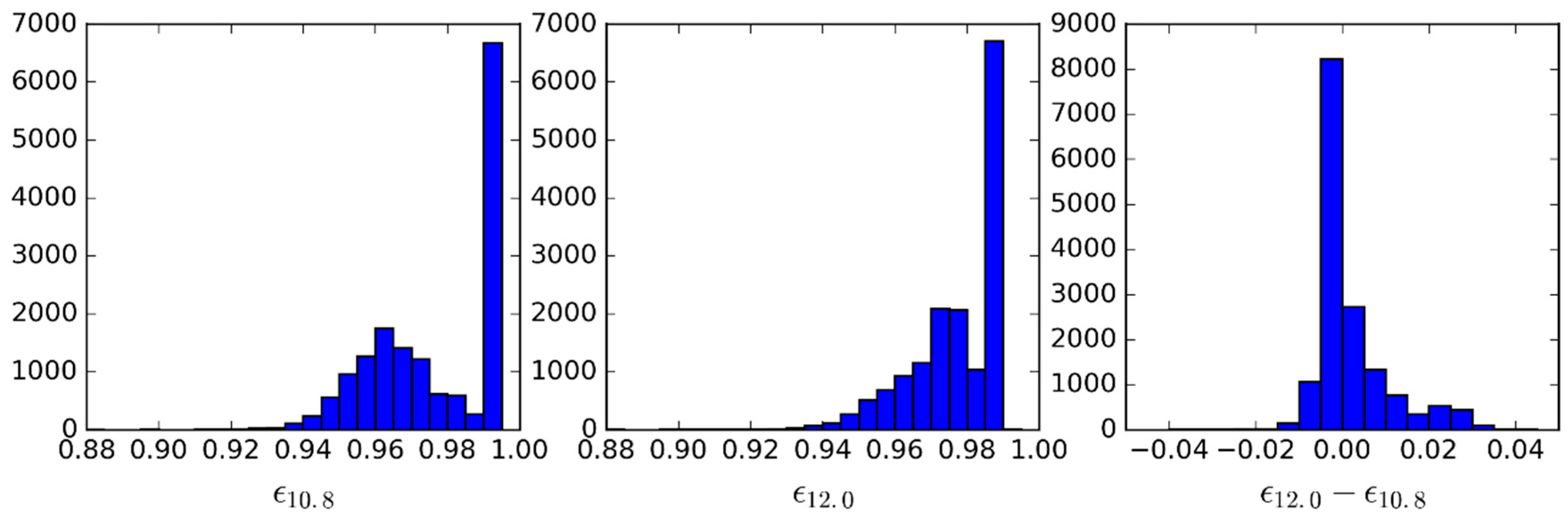
For the emissivity, a range of possible values are attributed to each of the cases above: values of ${ϵ}_{10.8}$ from 0.93 to 1.0 in steps of 0.01, and then, in the case of a GSW model, it is appropriate to prescribe departures from this value for ${ϵ}_{12.0}$: −0.015 to 0.035 in steps of 0.01 (excluding cases where ${ϵ}_{12.0}>1.0$), as suggested by Figure 4.

Figure 5 shows the statistical and geographical properties of the database gathered following those steps, which total 116 profiles. By combining these profiles with the prescribed viewing geometries and surface/low-level conditions proposed in steps 3 to 5, the total number of cases used in the calibration is 906,192. This number is around ten times larger than the number of simulations made for the validation dataset, which contains the remaining profiles in the SeeBor database, simulated with five random angles (within the ZVA range of each sensor) per profile. Note that the TCWV distribution (Figure 5a) is close to that of the whole SeeBor data set (Figure 2a), although moister profiles are relatively over-represented, so that a robust fit of LST algorithms can be achieved for these cases. Nevertheless, low humidity profiles still dominate within the distribution, to ensure a proper coverage of the $TCWV/T_{Skin}$ phase space (Figure 5c) and its large dynamic range of $T_{Skin}$ towards low TCWV values (as seen in Figure 2c).

The way the database is built also leads to a greater frequency of profiles gathered over land, since some of the most extreme conditions are only found there. The presence of some marine profiles is not problematic because algorithms also need to cover cases where the LST retrieval is made over small islands or coastal regions. Validation of LST products over large water bodies is also a common practice (e.g., [32]).

3. Results

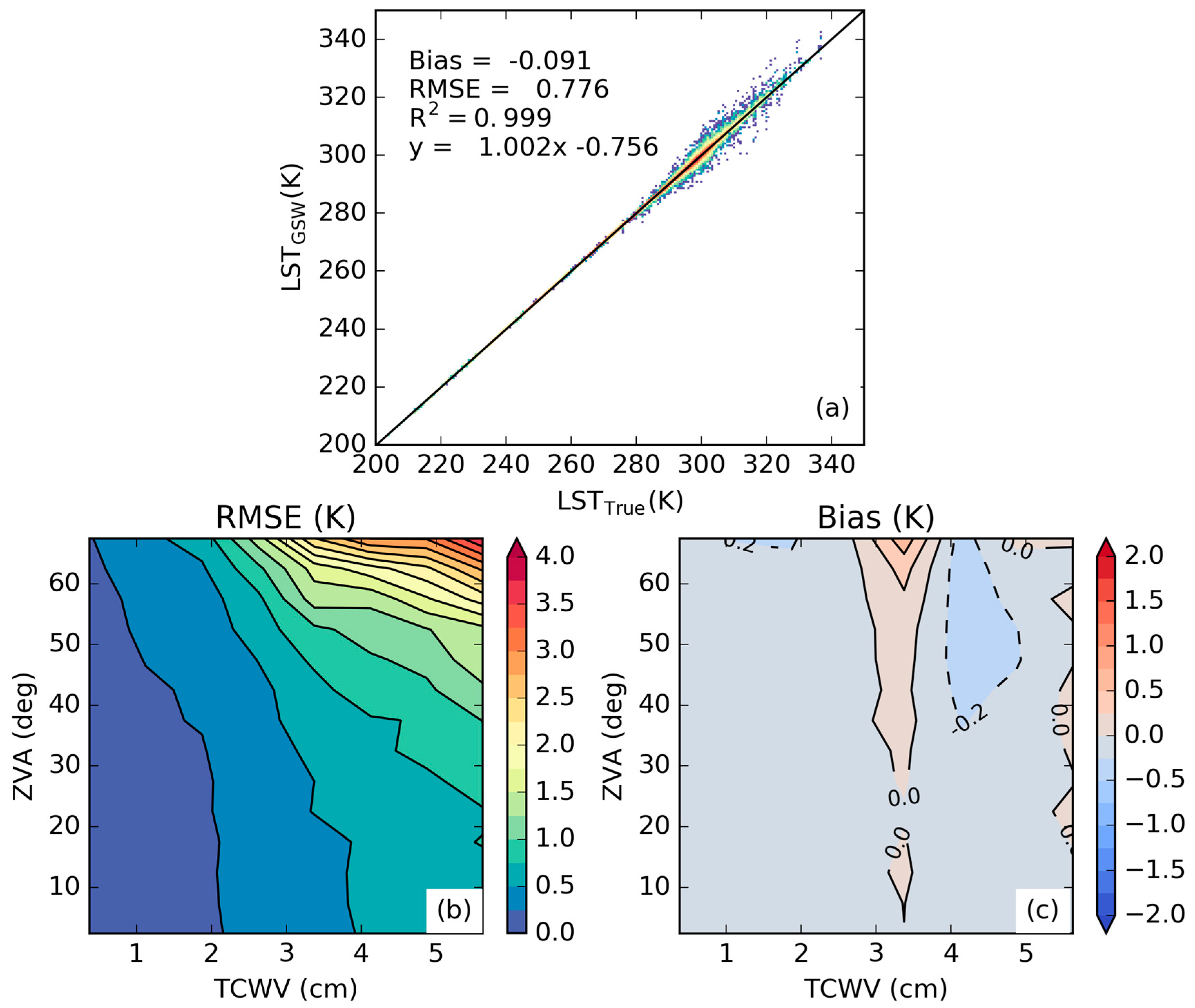
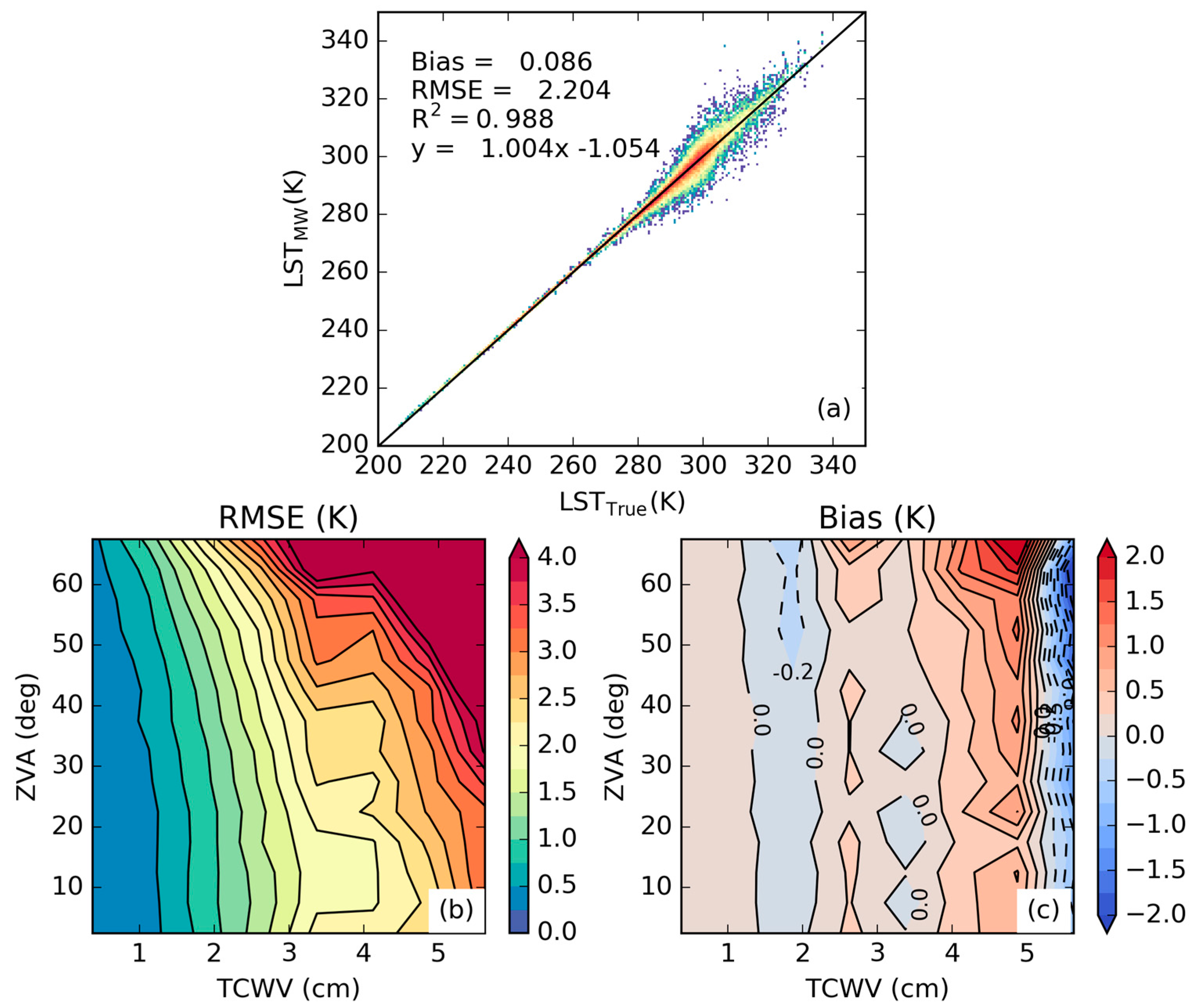
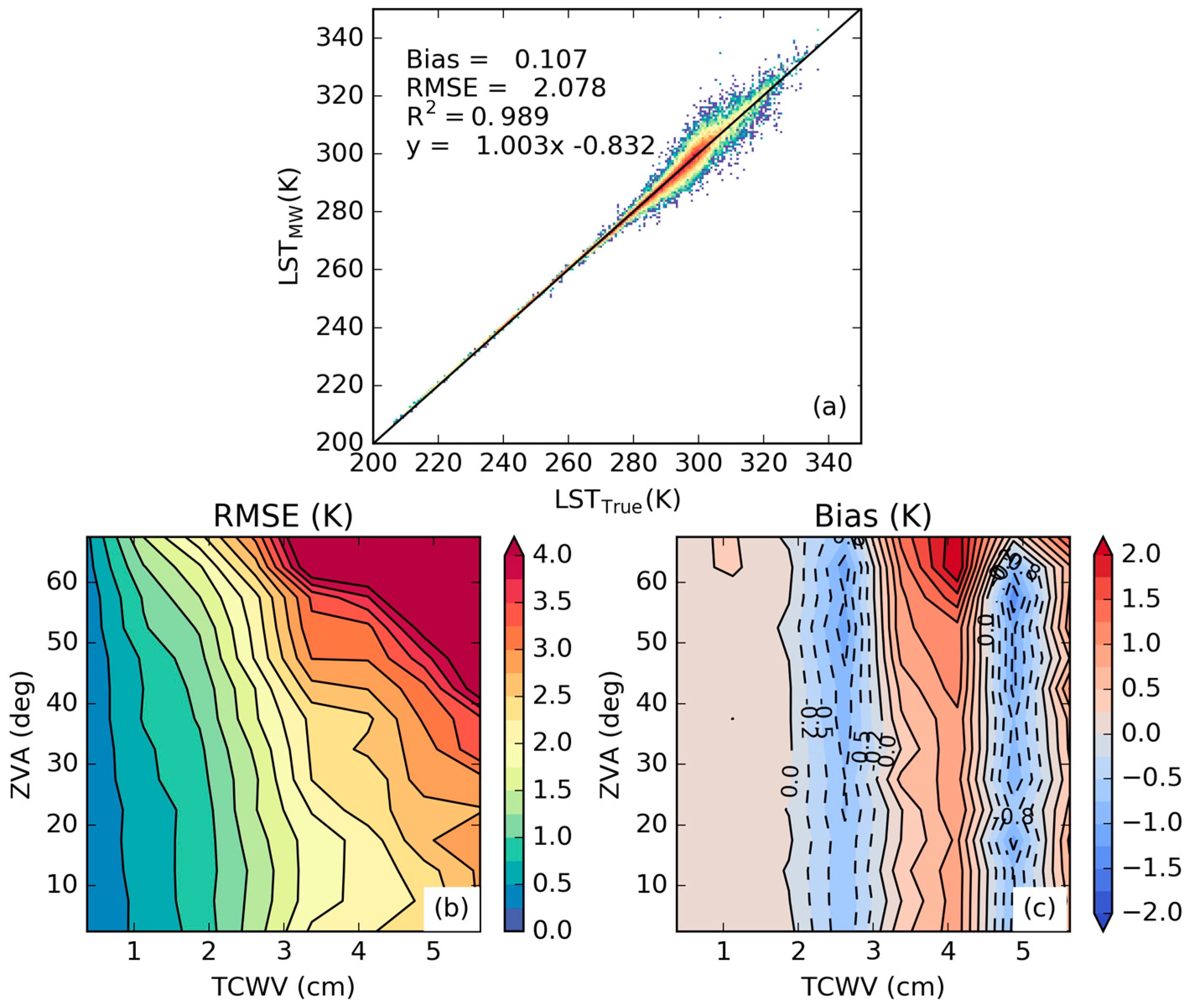
3.1. Error Statistics of the Proposed Calibration Database

Figure 6 shows the error statistics of the GSW algorithm adjusted using the proposed calibration database; the algorithm error (i.e., LST_GSW − LST_True) statistics are evaluated for the independent validation database. Globally, this reveals a bias of around −0.09 K and a Root Mean Square Error (RMSE) of 0.776 K, the scatterplot shows larger dispersions towards larger LSTs which is mainly caused by the greater water vapor content of such atmospheres. Especially when combined with large viewing angles, this kind of profile is responsible for the largest retrieval errors. This is confirmed by the diagram on the center of Figure 6 which shows the RMSE per class of ZVA and TCWV: larger RMSE values of above 3 K appear for classes with larger optical path (larger ZVA and larger TCWV). On the other hand, nearly all classes below 3 cm and below 50 degrees show RMSEs of 0.5 K or lower. The distribution of the bias over the TCWV/ZVA diagram shows that this statistic does not change much across the different classes with only a few classes with positive and negative biases of magnitudes around 0.2 K, towards higher values of TCWV.

In Figure 7 the same statistics are analyzed in the case of the MW model. Although this model shows nearly the same overall bias (0.086 K), its RMSE is almost three times larger (of about 2.20 K). The way the RMSE is distributed along the classes of TCWV and ZVA is much less linear than in the case of the GSW model and presents a stronger dependency on TCWV even for low ZVAs. Moreover, there are more classes with retrieval errors that are close to the limit acceptable for LST algorithms (e.g., LSA-SAF LST products consider 4 K to be their threshold accuracy requirement; [20]). The bias also has a more complex structure among the TCWV/ZVA classes, some of them reaching more than 1 K, both positive and negative showing that the overall bias results from the cancellation of values between different classes. The differences between Figure 6 and Figure 7, and in particular the steeper increase in RMSE with TCWV in the MW, emphasize the importance of using GSW-type schemes whenever possible.

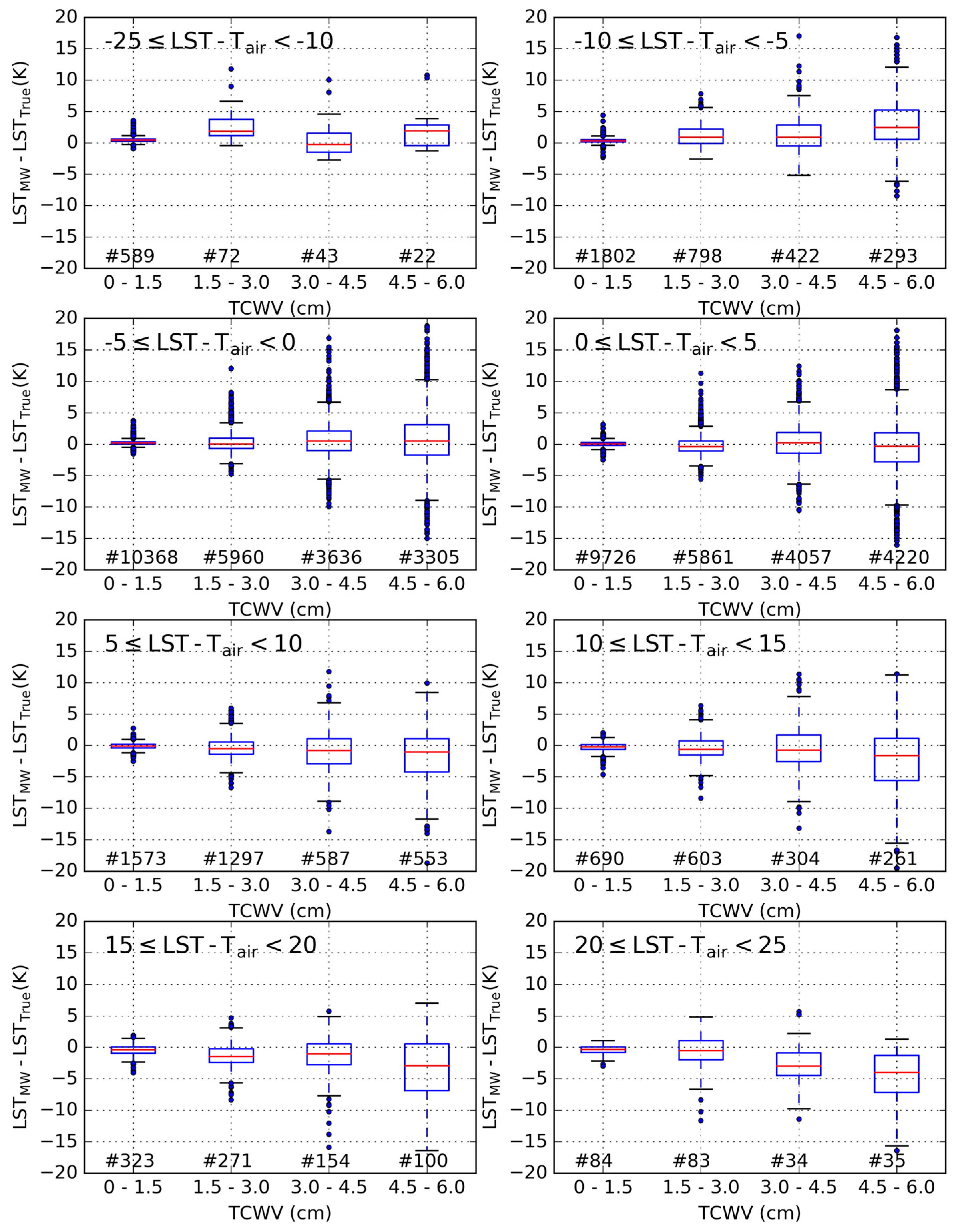
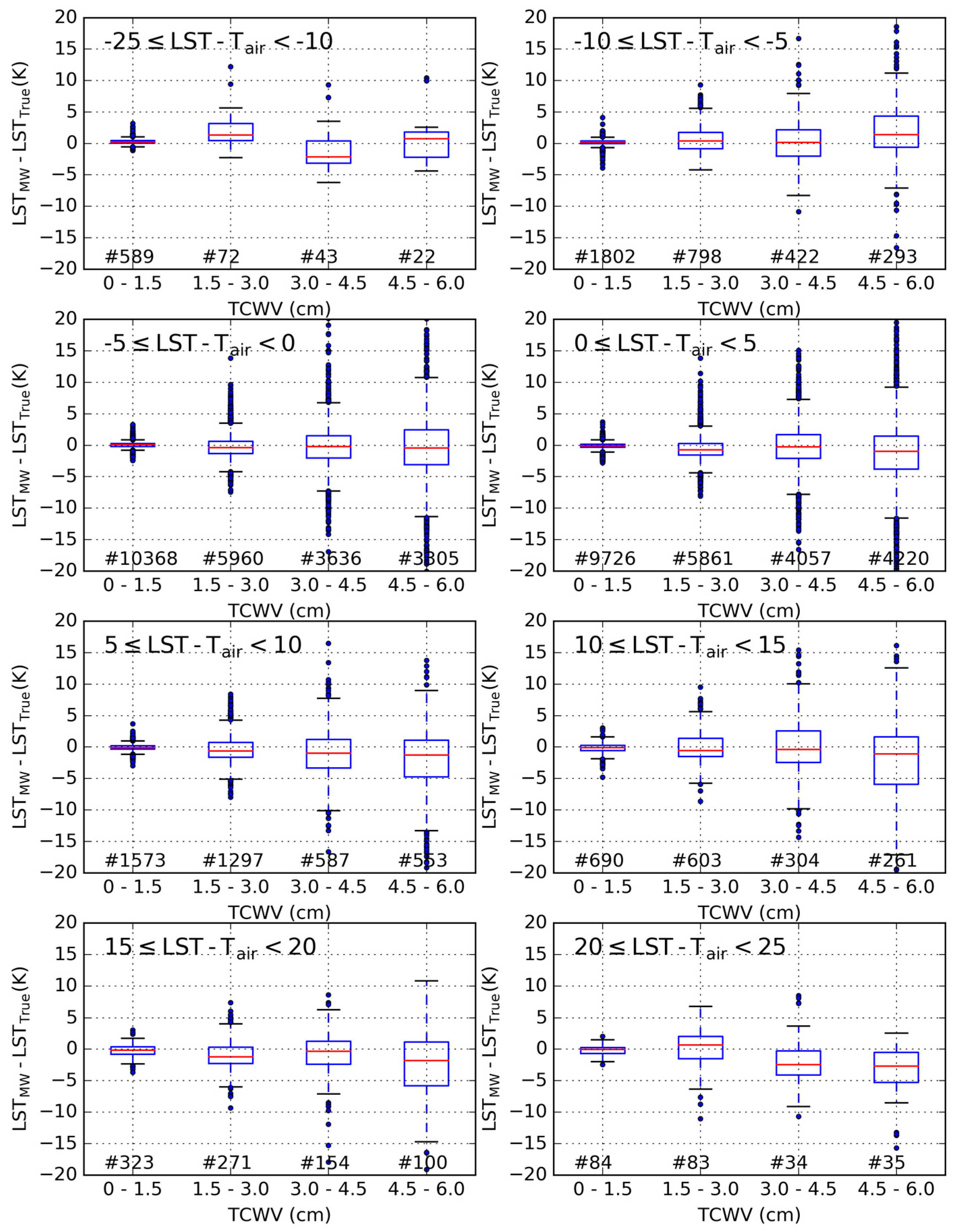
3.2. Sensitivity to the Distribution of Relevant Variables

In order to study the sensitivity of the proposed database to some of the choices that were made, a set of experiments was performed. The baseline calibration dataset, which is based on a choice of profiles that is adequate to fill the TCWV/LST diagram, is referred to as WTS_−15_15 (TCWV is sometimes represented as W in the literature and TS stands for $T_{Skin}$). A different criterion could have been adopted to choose a few calibration profiles from the more than 15000 profiles in the SeeBor database, such as ensuring a flat distribution of TCWV. This criterion was adopted, together with the wide geographical distribution criterion of WTS_−15_15, for experiments FLAT14_−15_15 and FLAT10_−15_15. The difference between these two is that for the first, 14 profiles per TCWV class were chosen (112 profiles vs. 116 in WTS_−15_15) and for the latter only 10 (leading to a total of 80 profiles). The goal was to test the relevance of the number of profiles and of the respective joint LST /TCWV distribution for the robustness of the regression coefficients. The statistical and geographical distributions of these databases are illustrated in Figure 8 and Figure 9. Large parts of the TCWV/LST diagram are not covered such as the most extreme LST classes. In the intermediate TCWV classes, a large number of the cases fall in the same LST range, as these combinations are globally more frequent for clear sky conditions, and therefore also more frequent in the SeeBor database. Note that a few of the profiles are common to FLAT14_−15_15 and to FLAT10_−15_15; this is because the algorithm is initiated with the same random seed, which generated the same random number sequence for all the experiments. The geographical distributions show that relatively fewer profiles over land are selected, which might be explained by the fact that the inclusion of more extreme situations was not a requirement.

Another factor that greatly influences the robustness of the coefficients is the $LST-T_{air}$ difference. Therefore, we tested a few variants of the WTS_−15_15 database varying the lower and upper limits of the prescribed $LST-T_{air}$ difference, always using steps of 5 K. These experiments are referred to as WTS_−10_10, WTS_−10_15, WTS_−10_20, WTS_−15_20, WTS_−20_15, WTS_−20_20, WTS_−20_25 and WTS_−25_25 (the numbers in the experiment name refer to the lower and upper limits of $LST-T_{air})$. All these choices of calibration databases were tested in both the GSW and the MW formulations and the same validation database was used to assess their statistical properties. The set of sensitivity experiments is described in

Table 1. Description of the calibration database sensitivity experiments.

Database	Selection of Profiles	Number of Profiles	Prescribed $\mathit{L}\mathit{S}\mathit{T}-{\mathit{T}}_{\mathit{a}\mathit{i}\mathit{r}}$ Range (K)
Baseline: WTS_−15_15	Full coverage of the LST/TCWV phase space	116	−15 to +15
FLAT14_−15_15	Flat distribution of TCWV with 14 profiles per TCWV class	112	−15 to +15
FLAT10_−15_15	Flat distribution of TCWV with 10 profiles per TCWV class	80	−15 to +15
WTS_−10_10	Full coverage of the LST/TCWV phase space	116	−10 to +10
WTS_−10_15	Full coverage of the LST/TCWV phase space	116	−10 to +15
WTS_−10_20	Full coverage of the LST/TCWV phase space	116	−10 to +20
WTS_−15_20	Full coverage of the LST/TCWV phase space	116	−15 to +20
WTS_−20_15	Full coverage of the LST/TCWV phase space	116	−20 to +15
WTS_−20_20	Full coverage of the LST/TCWV phase space	116	−20 to +20
WTS_−20_25	Full coverage of the LST/TCWV phase space	116	−20 to +25
WTS_−25_25	Full coverage of the LST/TCWV phase space	116	−25 to +25

.

The results of the sensitivity experiments are summarized in

Table 2. Error statistics for the sensitivity experiments. The bias is calculated by averaging the difference $LS{T}_{GSW}-LS{T}_{True}$ for the validation database. The database with the best statistic is highlighted in red.

Database	Bias (K)	RMSE (K)	Bias Stdev (K)	RMSE Stdev (K)
Baseline: WTS_−15_15	−0.09	0.78	0.14	0.67
FLAT14_−15_15	−0.12	0.81	0.38	0.70
FLAT10_−15_15	−0.11	0.82	0.32	0.72
WTS_−10_10	0.05	0.74	0.26	0.64
WTS_−10_15	0.07	0.76	0.34	0.69
WTS_−10_20	0.09	0.81	0.41	0.73
WTS_−15_20	−0.02	0.76	0.21	0.67
WTS_−20_15	−0.11	0.79	0.14	0.68
WTS_−20_20	−0.12	0.78	0.14	0.68
WTS_−20_25	−0.11	0.78	0.15	0.68
WTS_−25_25	−0.25	0.87	0.22	0.73

and

Table 3. Same as Table 2 but for the MW model.

Database	Bias (K)	RMSE (K)	Bias Stdev (K)	RMSE Stdev (K)
Baseline: WTS_−15_15	0.09	2.02	0.71	1.63
FLAT14_−15_15	0.11	2.08	0.73	1.42
FLAT10_−15_15	−0.04	2.05	0.69	1.38
WTS_−10_10	0.55	1.97	0.70	1.35
WTS_−10_15	0.76	2.19	0.92	1.54
WTS_−10_20	0.89	2.39	1.09	1.72
WTS_−15_20	0.43	2.28	0.83	1.69
WTS_−20_15	−0.13	2.23	0.71	1.67
WTS_−20_20	0.04	2.34	0.76	1.68
WTS_−20_25	0.16	2.46	0.83	1.89
WTS_−25_25	−0.28	2.67	0.89	2.07

for the GSW and MW algorithms, respectively. Both algorithms were adjusted using the different calibration databases described above and assessed using a common and independent validation database. In Table 2 and Table 3, values of the overall bias and RMSE are indicated, as well as their variability among the TCWV/ZVA classes (via the standard deviation of the bias and RMSE, respectively, obtained per TCWV/ZVA class). The GSW model shows a slightly higher bias and RMSE using the FLAT approach when compared to the WPS. Their variabilities are also larger for the FLAT-type databases, which means that there are classes that are not so well represented when using this approach.

The set of experiments summarized in Table 1 also suggest high sensitivity to the lower and upper limits of the prescribed $LST-T_{air}$ difference prescribed in the calibration databases as this range is the only condition changing among experiments denoted by “WTS”. The results presented in Table 1 suggest that it is hard to tell which combination is the best. In general, widening the $LST-T_{air}$ range of possible values seems to make the overall RMSE worse, although there are a few exceptions. Another discernible pattern regards the sign and magnitude of the overall bias: increasing the upper limit increases the bias (i.e., it becomes “more positive”); conversely, decreases in the lower limit seem to make the bias more negative. Well-balanced ranges (absolute value of the lower and the upper limits close to each other) seem to lower the variability of the statistics.

In the case of the MW model, the experiments show even less linear results. In fact, the case with more favorable error statistics is arguably FLAT10_−15_15, with a lower absolute value of the bias and bias variability, an overall RMSE that is comparable to that of the baseline experiment and with less variability among classes. For the MW model, the experiment with the smallest RMSE is WTS_−10_10 (of about 1.97 K); however, it has also the worst absolute value for the bias, 0.55 K. Like in the case of the GSW model, there is also a tendency to get worse RMSE values towards wider ranges of $LST-T_{air}$ difference.

These results suggest that the configuration of an appropriate calibration database may vary with the algorithm to be used and area coverage, as the distribution of the variables analyzed above (most notably $LST-T_{air}$) over the area of interest may support the exclusion of more extreme cases and non-relevant. The choice of profiles from a SeeBor-like database is non-trivial, but basing the choice on fully covering the bivariate TCWV/LST distribution over the respective region of interest seems to have some advantages. It is worth noting that covering the most frequent classes in the TCWV/LST diagram leads, as expected, to better overall statistics, as those will be the most frequent in the validation database (and also in real applications). In Figure 10, the overall statistics are analyzed for the FLAT14_−15_15 calibration database, which, despite having a comparable number of profiles to WTS_−15_15 and much more than FLAT10_−15_15, shows overall worse performance than those cases. The analysis of the bias (Figure 10c) as a function of TCWV clearly shows that some classes are affected by large negative biases (between 2 and 3 cm, and around 5 cm) while between 3 and 4 cm the bias is positive; the ZVA dependency seems less important in the analyzed case. This shows that even with a flat distribution of TCWV, the performance of the model will depend on the TCWV, suggesting that combined distributions of variables relevant to the problem need to be taken into account. In practice this would translate in a roughly latitude-dependent bias (following the latitude dependence of TCWV), which is something that should be avoided in global datasets.

In order to explore the effect of the prescribed $LST-T_{air}$ differences in the representation of the most extreme cases, boxplots of the error distribution (as given by $LS{T}_{MW}-LS{T}_{True}$) were calculated by classes of $LST-T_{air}$ in the validation database, and also as a function of the TCWV class, for two of the proposed experiments: MW calibrated using WTS_−15_15 and WTS_−25_25, respectively, as shown in Figure 11 and Figure 12. There were some classes with only few cases, reflecting the fact that largely negative differences rarely occur and they do so in very dry atmospheres, so we merged them into a single class $-25K\le LST-T_{air}<10K$ to increase the figure readability. Large positive differences are more frequent and may occur in all types of atmospheres. The comparison of the error distributions shown in Figure 11 and Figure 12 indicates that only a few classes seem to be statistically affected by the temperature difference range that is applied. In drier atmospheres (TCWV < 3 cm) the effect is in fact negligible, since under these conditions the TOA brightness temperatures will be highly dominated by the surface emitted signal (i.e., by LST and surface emissivity). In most cases, the only noticeable effect is the increase in the range of the error when the temperature difference increases, even in those classes that are “covered” by both calibration databases (e.g., $5 K\le LST-T_{air}<10 K$). This is what causes the overall loss of performance of the database with the wider temperature ranges, since those classes are more populated than those with more extreme temperature differences. It is also worth noticing that extending the temperature difference range does not necessarily lead to a better representation of the extreme cases. When $LST-T_{air}$ is positive and large, it likely means the surface sensible heat flux may generate a convective boundary layer, which is often topped by a temperature inversion [33]. It is well known that large LST retrieval errors occur under very moist atmospheres (e.g., [20]). If on top of such conditions we have the development of a convective boundary layer, the height of the largest thermal and moisture gradients may be shifted upwards and therefore the peak of thermal weighting function of (split-)window channels may also be shifted upwards [34,35,36], which makes it harder to disentangle surface emission (LST and emissivity) from the signal emitted by the lower atmosphere. Some currently used schemes address this issue using different coefficients for day and night retrievals (e.g., [37]), which somewhat tunes the LST algorithms to different structures of the atmospheric boundary layer but introduces an additional discontinuity in the algorithm coefficients, while other schemes use additional information from numerical weather prediction models regarding near-surface air temperature (which may also bring additional model forecast errors into the retrieval). Although not shown, the GSW model seems much less sensitive to these effects, as the boxplot diagrams for the cases illustrated in Figure 11 and Figure 12 for the MW algorithm are much closer to each other in the GSW case. In summary, extending the $LST-T_{air}$ values to include the most extreme cases may not be beneficial for the overall performance of the retrievals because it can lead to higher errors in the classes that are more frequent, without significant compensation from the classes with more extreme situations.

4. Conclusions

The problem of how to design a calibration database for semi-empirical retrieval methods for LST is addressed here by identifying the factors that may influence the quality of the calibration (and therefore of the retrieval) and then investigating their physical range of variability. Considering the equation of radiative transfer between the surface and the TOA within the thermal infrared window, particular attention should be paid to three main factors, namely: (1) the atmospheric transmissivity and its vertical structure, which in turn is conditioned by the water vapor profile, as the main absorber/emitter and most variable gas in the wavelengths of interest, together with the viewing geometry; (2) the surface emissivity and its spectral variations; and finally (3) the low level thermal structure of the atmosphere, which may affect the vertical level at which the sensor is more sensitive in the channels of interest.

Assuming that we would like to design algorithm calibration databases that would lead to good fit under all possible conditions, one of the main questions is whether it is possible to improve the representation of the most extreme cases without compromising the performance of the overall retrieval. In this work it is shown that the answer to this question is not trivial. The selection of a set of atmospheric profiles that spans the range of surface temperatures and total column water vapor combinations that are physically possible seems beneficial for the quality of the regression model, but only modestly. Nevertheless, this ensures that a thorough representation of the possible cases is achieved when the model coefficients are trained, thus avoiding biases in certain classes of input parameters or retrieval conditions. The effects are amplified when a MW model is used instead of a GSW.

In terms of the representation the thermal structure of the low-levels in the atmosphere, the situation is slightly more complex. The inclusion of more extreme temperature differences between the surface and the near-surface air in the calibration database, rather than restricting them to more frequent/moderate cases, degrades the performance of the models especially under moist atmospheres, on which atmospheric emission is non-negligible. Also, such atmospheres are often characterized by well-developed boundary layers and as such, temperature inversions and strong vertical gradients may be present, complicating the atmospheric correction problem. Fully addressing this issue is left for future work.

Regardless of the calibration database used, the errors of LST estimations obtained for an independent validation database can be used to fully characterize the uncertainty of the LST algorithm, which heavily depends on retrieval conditions. The uncertainty budget of LST satellite products will then be the result of that of the algorithm together with the propagation of input uncertainties.

This article summarizes the procedure currently in practice within the EUMETSAT LSA SAF to calibrate the retrieval algorithms for a variety of LST products. The previously used methodology [20] gathered experience from a number of studies (e.g., [16,21,38,39]) but missed an objective criterion to physically constrain the selection of profiles used for calibration, which leads to an algorithm with lower uncertainty. The methodology designated here as WTS_−15_15 is a good compromise addressing the widest possible retrieval conditions, which is a pre-requisite for a global LST product. Future LST products, especially with inputs from the Flexible Combined Imager on board Meteosat Third Generation [24] will benefit from the knowledge provided by this study. It is possible, though, that for different applications (e.g., regional LST products) a different choice of calibration database is more suitable. As such, LST developers should consider the joint distributions of the relevant variables, as detailed above, for their area of interest and to perform similar sensitivity analyses to their algorithms.

References

- Dirmeyer, P.A.; Cash, B.A.; Kinter, J.L.; Stan, C.; Jung, T.; Marx, L.; Towers, P.; Wedi, N.; Adams, J.M.; Altshuler, E.L.; et al. Evidence for enhanced land-atmosphere feedback in a warming climate. J. Hydrometeorol. 2012, 13, 981–995. [Google Scholar] [CrossRef]
- Wan, Z.; Wang, P.; Li, X. Using MODIS land surface temperature and normalized difference vegetation index products for monitoring drought in the southern Great Plains, USA. Int. J. Remote Sens. 2004, 25, 61–72. [Google Scholar] [CrossRef]
- Guillod, B.P.; Orlowsky, B.; Miralles, D.G.; Teuling, A.J.; Seneviratne, S.I. Reconciling spatial and temporal soil moisture effects on afternoon rainfall. Nat. Commun. 2015, 6, 6443. [Google Scholar] [CrossRef] [PubMed] [Green Version]
- Kustas, W.P.; Norman, J.M. Use of remote sensing for evapotranspiration monitoring over land surfaces. Hydrol. Sci. J. 1996, 41, 495–516. [Google Scholar] [CrossRef]
- Taylor, C.M.; Gounou, A.; Guichard, F.F.; Harris, P.P.; Ellis, R.J.; Couvreux, F.; De Kauwe, M. Frequency of sahelian storm initiation enhanced over mesoscale soil-moisture patterns. Nat. Geosci. 2011, 4, 430–433. [Google Scholar] [CrossRef] [Green Version]
- Trigo, I.F.; Viterbo, P. Clear-sky window channel radiances: A comparison between observations and the ECMWF model. J. Appl. Meteorol. 2003, 42, 1463–1479. [Google Scholar] [CrossRef]
- Trigo, I.F.; Boussetta, S.; Viterbo, P.; Balsamo, G.; Beljaars, A.; Sandu, I. Comparison of model land skin temperature with remotely sensed estimates and assessment of surface-atmosphere coupling. J. Geophys. Res. Atmos. 2015, 120, 12096–12111. [Google Scholar] [CrossRef]
- Wang, A.; Barlage, M.; Zeng, X.; Draper, C.S. Comparison of land skin temperature from a land model, remote sensing, and in situ measurement. J. Geophys. Res. Atmos. 2014, 119, 3093–3106. [Google Scholar] [CrossRef]
- Zheng, W.; Wei, H.; Wang, Z.; Zeng, X.; Meng, J.; Ek, M.; Mitchell, K.; Derber, J. Improvement of daytime land surface skin temperature over arid regions in the NCEP GFS model and its impact on satellite data assimilation. J. Geophys. Res. Atmos. 2012, 117, D06117. [Google Scholar] [CrossRef]
- Caparrini, F.; Castelli, F.; Entekhabi, D. Variational estimation of soil and vegetation turbulent transfer and heat flux parameters from sequences of multisensor imagery. Water Resour. Res. 2004, 40, 1–15. [Google Scholar] [CrossRef]
- English, S.J. The importance of accurate skin temperature in assimilating radiances from satellite sounding instruments. IEEE Trans. Geosci. Remote Sens. 2008, 46, 403–408. [Google Scholar] [CrossRef]
- Ghent, D.; Kaduk, J.; Remedios, J.; Ardö, J.; Balzter, H. Assimilation of land surface temperature into the land surface model JULES with an ensemble Kalman filter. J. Geophys. Res. 2010, 115, D19112. [Google Scholar] [CrossRef]
- Li, Z.L.; Tang, B.H.; Wu, H.; Ren, H.; Yan, G.; Wan, Z.; Trigo, I.F.; Sobrino, J.A. Satellite-derived land surface temperature: Current status and perspectives. Remote Sens. Environ. 2013, 131, 14–37. [Google Scholar] [CrossRef]
- Trigo, I.F.; Peres, L.F.; DaCamara, C.C.; Freitas, S.C. Thermal land surface emissivity retrieved from SEVIRI/Meteosat. IEEE Trans. Geosci. Remote Sens. 2008, 46, 307–315. [Google Scholar] [CrossRef]
- Freitas, S.C.; Trigo, I.F.; Macedo, J.; Barroso, C.; Silva, R.; Perdigão, R. Land surface temperature from multiple geostationary satellites. Int. J. Remote Sens. 2013, 34, 3051–3068. [Google Scholar] [CrossRef]
- Sun, D.; Pinker, R.T. Estimation of land surface temperature from a geostationary operational environmental satellite (GOES-8). J. Geophys. Res. 2003, 108, 4326. [Google Scholar] [CrossRef]
- Duguay-Tetzlaff, A.; Bento, V.; Göttsche, F.; Stöckli, R.; Martins, J.; Trigo, I.; Olesen, F.; Bojanowski, J.; da Camara, C.; Kunz, H. Meteosat land surface temperature climate data record: Achievable accuracy and potential uncertainties. Remote Sens. 2015, 7, 13139–13156. [Google Scholar] [CrossRef]
- Jiménez-Muñoz, J.C. A generalized single-channel method for retrieving land surface temperature from remote sensing data. J. Geophys. Res. 2003, 108, 4688. [Google Scholar] [CrossRef]
- Sobrino, J.A.; Jiménez-Muñoz, J.C. Land surface temperature retrieval from thermal infrared data: An assessment in the context of the Surface Processes and Ecosystem Changes Through Response Analysis (SPECTRA) mission. J. Geophys. Res. D Atmos. 2005, 110, 1–10. [Google Scholar] [CrossRef]
- Freitas, S.C.; Trigo, I.F.; Bioucas-dias, J.M.; Göttsche, F. Quantifying the uncertainty of land surface temperature retrievals from SEVIRI/Meteosat. IEEE Trans. Geosci. Remote Sens. 2010, 48, 523–534. [Google Scholar] [CrossRef]
- Wan, Z.; Dozier, J. A generalized split-window algorithm for retrieving land-surface temperature from space. IEEE Trans. Geosci. Remote Sens. 1996, 34, 892–905. [Google Scholar]
- Mattar, C.; Durán-Alarcón, C.; Jiménez-Muñoz, J.C.; Santamaría-Artigas, A.; Olivera-Guerra, L.; Sobrino, J.A. Global atmospheric profiles from reanalysis information (GAPRI): A new database for earth surface temperature retrieval. Int. J. Remote Sens. 2015, 36, 5045–5060. [Google Scholar] [CrossRef]
- Trigo, I.F.; Dacamara, C.C.; Viterbo, P.; Roujean, J.L.; Olesen, F.; Barroso, C.; Camacho-de-Coca, F.; Carrer, D.; Freitas, S.C.; García-Haro, J.; et al. The satellite application facility for land surface analysis. Int. J. Remote Sens. 2011, 32, 2725–2744. [Google Scholar] [CrossRef]
- De La Taille, L.; Rota, S.; Hartley, C.; Stuhlmann, R. Meteosat third generation programme status. In Proceedings of the Annual EUMETSAT Meteorological Satellite Conference, Toulouse, France, 21–25 September 2015.
- Yu, Y.; Privette, J.L.; Pinheiro, A.C. Evaluation of split-window land surface temperature algorithms for generating climate data records. IEEE Trans. Geosci. Remote Sens. 2008, 46, 179–192. [Google Scholar] [CrossRef]
- Brutsaert, W. Hydrology: An Introduction; Cambridge Univ. Press: Cambridge, UK, 2005. [Google Scholar]
- Crago, R.D.; Qualls, R.J. Use of land surface temperature to estimate surface energy fluxes: Contributions of Wilfried Brutsaert and collaborators. Water Resour. Res. 2014, 50, 3396–3408. [Google Scholar] [CrossRef]
- Hulley, G.C.; Hook, S.J.; Abbott, E.; Malakar, N.; Islam, T.; Abrams, M. The ASTER Global Emissivity Dataset (ASTER GED): Mapping earth’s emissivity at 100 meter spatial scale. Geophys. Res. Lett. 2015, 42, 7966–7976. [Google Scholar] [CrossRef]
- Bulgin, C.E.; Embury, O.; Merchant, C.J. Sampling uncertainty in gridded sea surface temperature products and Advanced Very High Resolution Radiometer (AVHRR) Global Area Coverage (GAC) data. Remote Sens. Environ. 2016, 177, 287–294. [Google Scholar] [CrossRef]
- Berk, A.; Anderson, G.P.; Bernstein, L.S.; Acharya, P.K.; Dothe, H.; Matthew, M.W.; Adler-Golden, S.M.; Chetwynd, J.H., Jr.; Richtsmeier, S.C.; Pukall, B.; et al. MODTRAN4 radiative transfer modeling for atmospheric correction. Proc. SPIE 1999, 3756, 348–353. [Google Scholar]
- Borbas, E.E.; Seemann, S.W.; Huang, H.L.; Li, J.; Menzel, W.P. Global profile training database for satellite regression retrievals with estimates of skin temperature and emissivity. In Proceedings of International TOVS Study Conference-XIV, Beijing, China, 25–31 May 2005.
- Wan, Z. New refinements and validation of the MODIS land-surface temperature/emissivity products. Remote Sens. Environ. 2008, 112, 59–74. [Google Scholar] [CrossRef]
- Stull, R.B. An Introduction to Boundary Layer Meteorology; Kluwer Academic: Dordrecht, The Netherlands, 1988; p. 666. [Google Scholar]
- Rodgers, C.D. Inverse Methods for Atmospheric Sounding: Theory and Practice; World Scientific: Hackensack, NV, USA, 2000; Volume 2. [Google Scholar]
- Maddy, E.S.; Member, A.; Barnet, C.D. Vertical resolution estimates in version 5 of AIRS operational retrievals. IEEE Trans. Geosci. Remote Sens. 2008, 46, 2375–2384. [Google Scholar] [CrossRef]
- Martins, J.P.A.; Teixeira, J.; Soares, P.M.M.; Miranda, P.M.A.; Kahn, B.H.; Dang, V.T.; Irion, F.W.; Fetzer, E.J.; Fishbein, E. Infrared sounding of the trade-wind boundary layer: AIRS and the RICO experiment. Geophys. Res. Lett. 2010, 37. [Google Scholar] [CrossRef]
- Yu, Y.; Tarpley, D.; Privette, J.L.; Goldberg, M.D.; Rama Varma Raja, M.K.; Vinnikov, K.Y.; Xu, H. Developing algorithm for operational GOES-R land surface temperature product. IEEE Trans. Geosci. Remote Sens. 2009, 47, 936–951. [Google Scholar]
- Jiménez-Muñoz, J.C.; Sobrino, J.A. Error sources on the land surface temperature retrieved from thermal infrared single channel remote sensing data. Int. J. Remote Sens. 2006, 27, 999–1014. [Google Scholar] [CrossRef]
- Trigo, I.F.; Monteiro, I.T.; Olesen, F.; Kabsch, E. An assessment of remotely sensed land surface temperature. J. Geophys. Res. 2008, 113. [Google Scholar] [CrossRef]