Flash Flood Monitoring with an Inclined Lidar Installed at a River Bank: Proof of Concept

Abstract

Flash floods need to be monitored from a safe place, ideally with noncontact instruments installed at a riverbank and oriented so that they look obliquely at the water surface. The “inclined Lidar” technique could be useful for this purpose. It works based on the fact that a near-infrared Lidar mounted with a large incidence angle can detect suspended particles slightly below the surface, provided that the water is very turbid, something which is likely during flash floods. To check this hypothesis, an inexpensive “time of flight” (TOF) Lidar was installed during a rainy season at the Amacuzac River (Mexico), which was usually found to be extremely turbid (Secchi depth < 0.5 m). Under these circumstances, the Lidar had no difficulty detecting the water (sub) surface. Converting the measured distances into stage estimates through a simple (one point) calibration resulted in reasonable agreement with reference data (within ±0.08 m (p = 0.95) and always <0.5 m), especially during the passing of a flash flood. This is the first evidence that an inclined (TOF) Lidar can be used to monitor the stage during a flash flood. Indirectly, it also shows that a (Doppler) Lidar could be used to monitor water velocity during this type of event.

1. Introduction

Flash floods are a type of natural disaster which is quite common worldwide and very dangerous [1]. Most occur at the outlet of small catchments as a fast hydrological response to a storm (response time within less than a few hours) [2]. These floods need to be monitored in order to develop more efficient early warning systems through the calibration of rainfall–runoff models [2], set up of direct alert systems in particular cases [3], and investigation of long-term trends in river flooding [4].

Unfortunately, it is difficult to monitor flash floods in rivers using conventional hydrometric techniques. The main reason is that their installation requires a structure close to the riverbed (a stilling well, a bridge, or a mast [5,6]), which can be destroyed during the passing of a flash flood. Therefore, it would be useful to develop techniques that can monitor rivers from a safe place (i.e., far enough from the riverbed). Such techniques would ideally use noncontact instruments that can be installed at the riverbank (e.g., on the roof of a building with a line-of-sight to the river) and that can look at the water surface with a large incidence angle (typically larger than ≈60°). This would not only reduce the risk of damage in the event of a flood, but also the costs of installation and maintenance (e.g., [7]). It would also minimize the risk of vandalism (e.g., [8]).

A few hydrometric techniques to monitor flash floods are emerging. One of those is “large-scale particle image velocimetry” (LS-PIV), which detects certain contrasts at the water surface (passive remote sensing) [9,10]. However, it is still difficult to set up at night [11,12]. Another is microwave Radar (active remote sensing), which detects roughness at the water surface (due to the “Bragg resonance” phenomenon, which will certainly occur during a flood) [13,14]. Nevertheless, there is still a need to better understand how a Radar responds to the roughness produced by the underlying current (something different than the roughness produced by the wind, which is well known) [15]. As an alternative, this study focuses on the “inclined Lidar” technique [16], which works only when water is very turbid: a situation likely to happen during flash floods (e.g., [2]), as discussed more in detail at the end of the study.

2. Background

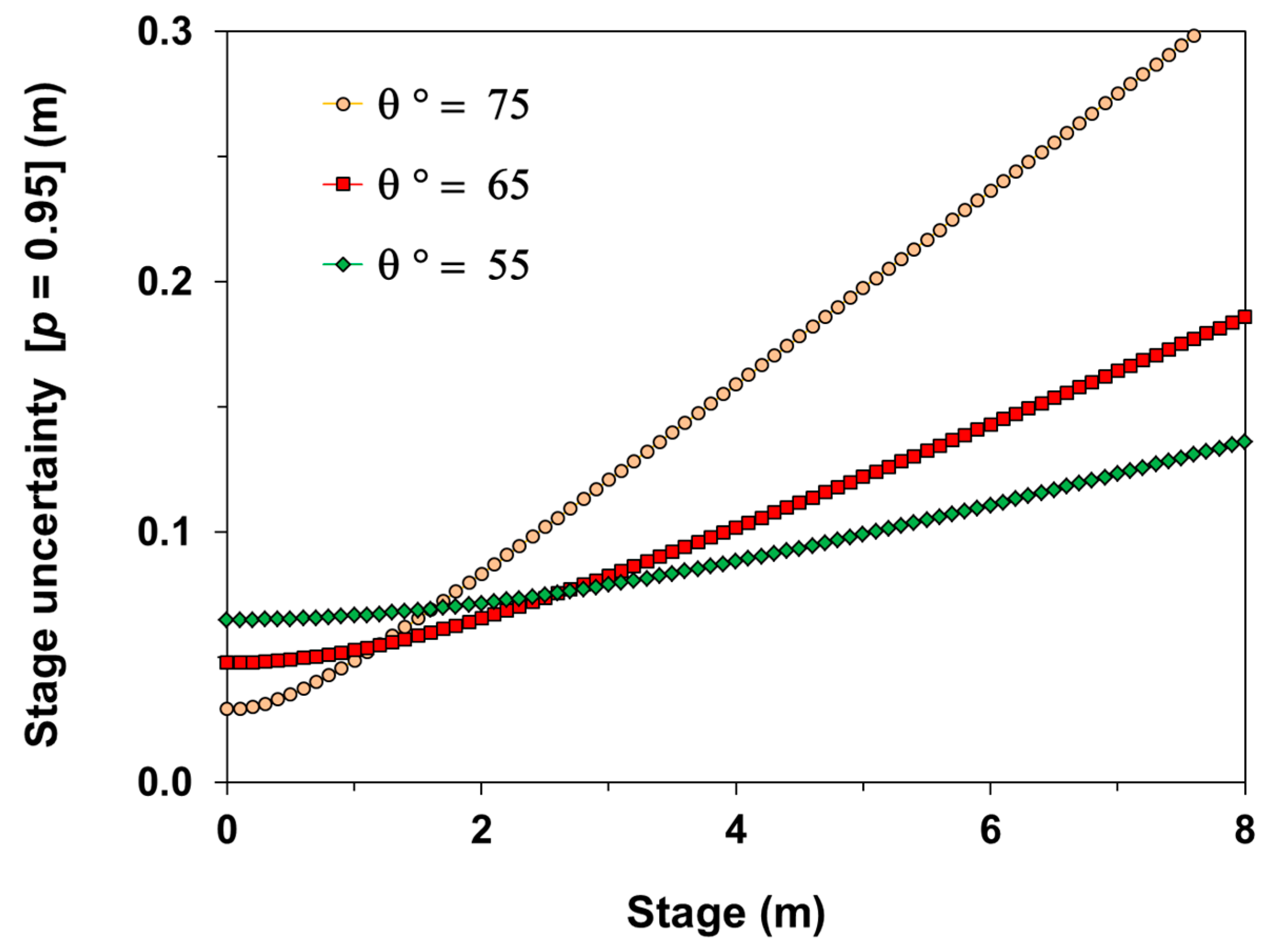
2.1. Stage Estimation

The inclined Lidar technique is based on the fact that a near-infrared Lidar mounted with a large incidence angle (between ≈30° and 70°) can detect suspended particles (due to the Tyndall effect) that are slightly below the surface, provided that water is turbid enough [16]. In this case, the distance to the detected particles can be measured with the “time of flight” (TOF) method, and this measurement can be easily used to compute a stage surrogate:

$$H=H_0-D\times \cos \left(\theta \right)$$

(1)

where H (m) is the stage, H₀ (m) is the height of the laser above a reference level (i.e., the river bottom in this study), D (m) is the distance measured by the Lidar, and θ (°) is the Lidar incidence angle.

2.2. One-Point Calibration

According to Equation 1, the Lidar incidence angle (θ) and its position above the river bottom (H₀) must be known in order to estimate stage data. As shown in a previous study [16], both parameters can be obtained empirically through calibration when at least two reference stage data are available. However, it is difficult to obtain reference stage data during the passing of a flash flood. In this case, a simple (one-point) calibration procedure was considered: (1) the Lidar incidence angle (θ) is not adjusted but rather measured (using an inclinometer); and (2) only the Lidar position above the river bottom (H₀) is adjusted, so that the Lidar stage estimations coincide with one reference stage data taken during a low-water period (H ≈ 0). This is equivalent to estimating the stage as: H = (D_max − D) × cos(θ), where D_max = H₀/cos(θ) is the distance between the Lidar and the river bottom (which is adjusted). In this case, the uncertainty of the Lidar stage estimates is given by [17]:

$$U\left(H\right)\approx \sqrt{2\times cos{\left(\theta \right)}^2\times U{\left(D\right)}^2+H^2\times tg{\left(\theta \right)}^2\times U{\left(\theta \right)}^2}$$

(2)

where U(•) denotes the expanded uncertainty (p = 0.95) (please note that in the formula θ must be expressed in radians). It is worth noting that the formula does not depend on the distance of the Lidar to the water surface (D) (i.e., the instrument can be installed at tenths of meters from the river without losing its accuracy).

As an example of application, let us consider: U(D) = 0.08 m and U(θ) = 0.01 rad (≈0.6°), which can easily be attained in practice [16]. In this case, and for a Lidar with an incidence angle of θ = 65°, the uncertainty of the stage estimates should be 0.05 m during low-water periods and should increase up to ≈0.15 m if the stage reaches 6 m (Figure 1), which is an extreme case (return period > 50 years) for the river described herein. Although this is not accurate compared to conventional stage monitoring techniques (e.g., [5]), the inclined Lidar technique is still attractive for monitoring flash floods due to its ease of implementation.

3. Materials and Methods

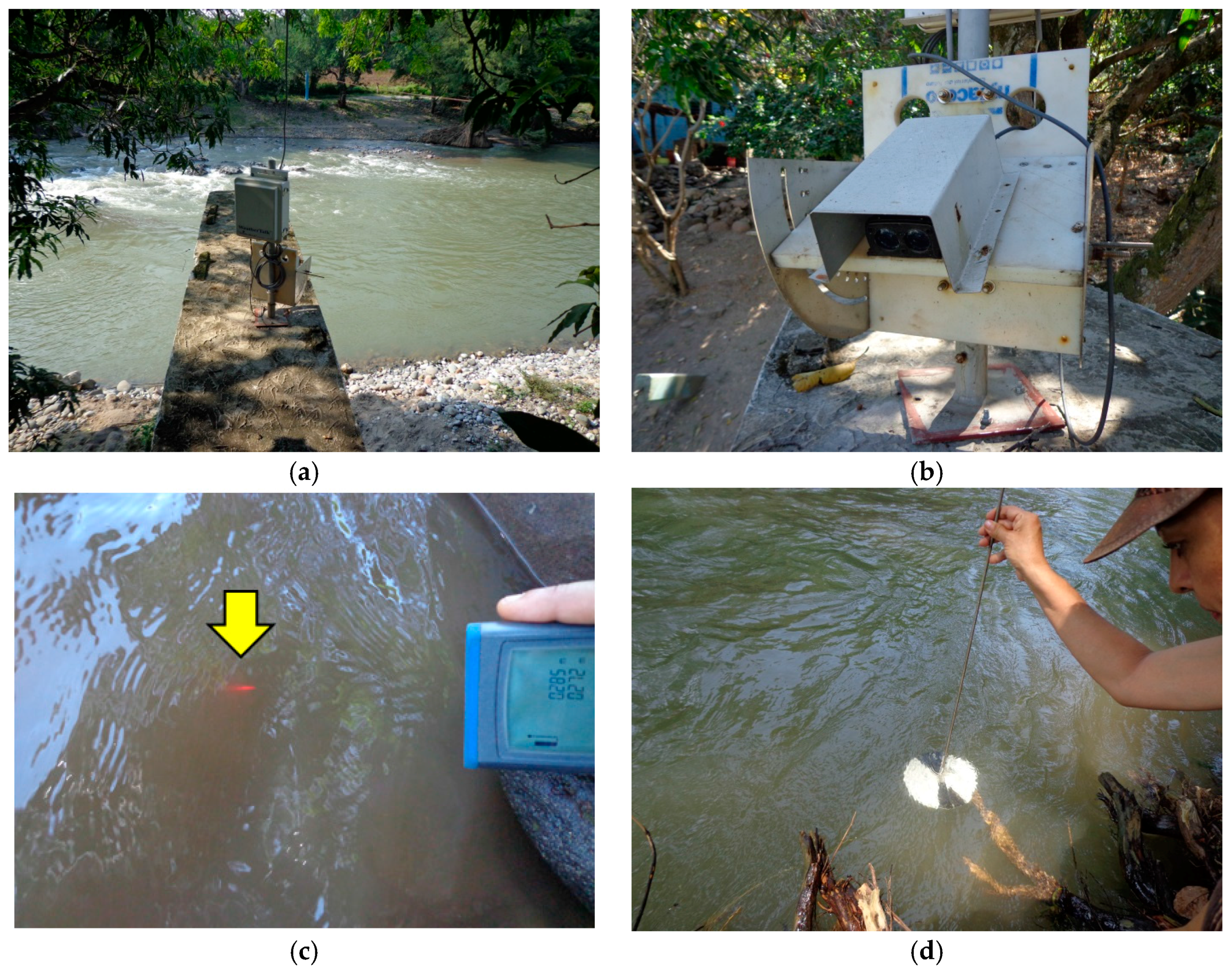
3.1. Test Lidar

The test Lidar (“TruSense S200”, Laser Technology Inc., Centennial, CO, USA) is an inexpensive instrument (≈1500 USD), which was used in a previous study [16]. It is a near-infrared (λ = 905 nm), safe-eye (class 1M) laser rangefinder with two refinements. On the one hand, it has three different modes to measure distance: “first pulse”, “strongest pulse”, and “last pulse”; according to the manufacturer [18], the last two modes can be useful to discriminate a target when there are translucent objects in the line-of-sight of the Lidar (e.g., mosquitoes, smog, rain and water surface). On the other hand, the Lidar returns a “signal strength” value associated with each distance data. Basically, this is an integer (I) which increases from 1 to 4 as the intensity of the laser pulses that are backscattered to the Lidar detector increases. Assuming that the signal strength depends mostly on the target reflectance (for a given Lidar configuration), its value was used to analyze the raw Lidar data.

As done by a previous study [16], the Lidar was configured to attempt to take distance data by sequentially using each one of the three available measurement modes. Each attempt consisted of a burst of 12 laser pulses, and in the case of a failed measurement, the Lidar was allowed to try again until reaching a maximum number of 16 attempts. It is worth noting that the Lidar was always left unsupervised while taking distance data; that is, regardless of what had been measured before and of what could be considered a priori as realistic.

3.2. Monitoring Campaign

To determine whether an inclined Lidar can be used to detect flash floods, an experiment was performed at a gauging station (18°35′48.61″N–99°22′38.14″W) located on the upper part of the Amacuzac River (Morelos state, Mexico). Because this site is the outlet of a rather small (2200 km²) mountainous catchment, it is characterized by flash floods (although not as violent as in other places). The test Lidar was installed on the river bank (Figure 2a,b), so that it was pointing at the water surface with an incidence angle (θ) of 64° (measured with a bubble inclinometer). As mentioned, the Lidar position above the river bottom (H₀) was adjusted during a low-water period.

A conventional technique was used as a reference for the stage monitoring: this consisted of a Radar (“RLS”, OTT Hydrometry, Kempten, Germany) mounted vertically on a bridge crossing the river. According to an intercomparison performed with another Radar (“Nile 502”, Waterlog, Yellow Springs, OH, USA) and two bubbling systems installed on the bridge during the experiment [6], the uncertainty of the reference data was ±0.02 m (p = 0.95) when the stage was <2.5 m.

For practical reasons, the Lidar and the Radar footprints could not be matched exactly: the Lidar was looking about 70 m upstream from the bridge where the Radar was installed. Once configured, the inclined Lidar and the conventional Radar were left to monitor the stage every 5 min during the end of a rainy season (September–November 2015). To assess the performances of the inclined Lidar technique (Figure 2c,d), the water transparency in the river was measured each week, using a Secchi disk [19].

4. Results

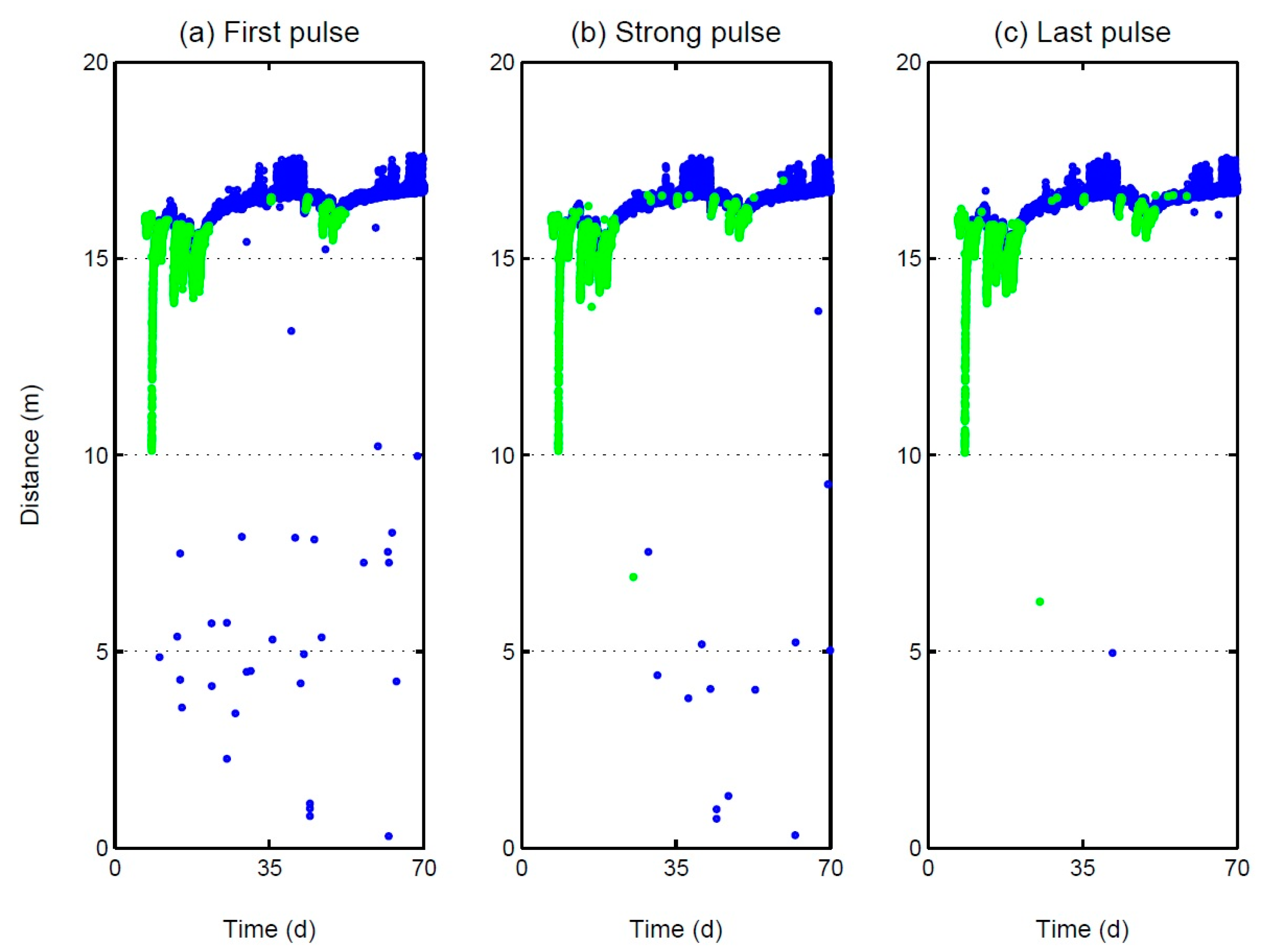
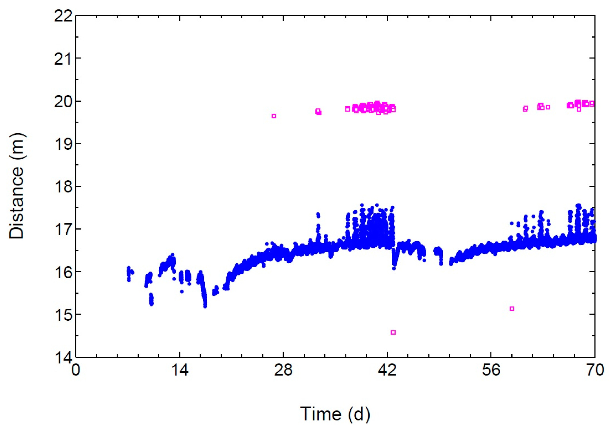
4.1. Raw-Data Processing

Previous studies performed with an inclined Lidar pointing at a turbid water surface (e.g., [16]) have shown that the raw distance data recorded by the Lidar can be very erratic. However, in the case of the test Lidar, it was empirically found that the raw distance data can be easily filtered according to their associated signal strength: a high signal strength (I = 4) was usually consistent with the detection of floating objects or an extremely turbid water (sub) surface (Secchi depth smaller than ≈0.5 m), a moderate intensity (I = 3) was usually consistent with the detection of a very turbid water (sub) surface (Secchi depth between 0.5 and 1.0 m), and a lower signal strength (I = 2) was related with the detection of less obvious features (see Appendix A). Although not as much as during a previous study performed in two turbid reservoirs [16], the raw distance data recorded by the test Lidar at the Amacuzac River were still erratic (Figure 3). Additionally, as expected, the distance data associated with a moderate (I = 3) or high (I = 4) signal strength were usually consistent with the detection of a water (sub) surface. So, these data were used to estimate the stage with the inclined Lidar technique.

In a previous study performed in two turbid reservoirs with the test Lidar [16], the “strongest pulse” mode was empirically found to be the best Lidar configuration because it provided more distance data related to the water (sub) surface. In addition, regrouping and filtering these data on a daily basis was proposed to reduce the noise in the raw distance data. However, when the goal is to monitor flash floods, it is of course essential to be able to register data with a good temporal resolution. Fortunately, the raw Lidar data recorded at the Amacuzac River were less noisy and less sensitive to the configuration mode of the instrument, which can be explained by extreme turbid conditions (as shown below). This made it possible to filter the instantaneous Lidar data according to a simple rule based on the three configuration modes. Specifically, a “good” distance data was computed each time as the median of the raw distance data obtained with the “first”, “strongest”, and “last” pulse modes, provided that (1) each raw data was associated with a moderate (I = 3) or high (I = 4) signal strength and that (2) the maximum difference between the three distance data was small (less than 0.12 m, i.e., three times the standard uncertainty of the distance measurements); if these conditions were not met, the inclined Lidar technique was considered to be unable to provide a “good” distance data (and therefore to estimate the stage) for a given time. The proposed rule is robust because it attempts to estimate each stage data independently of what has been estimated before and of what could be considered a priori as realistic.

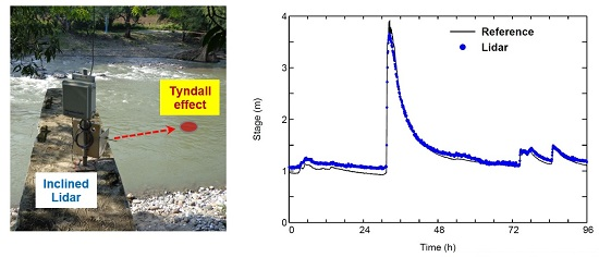
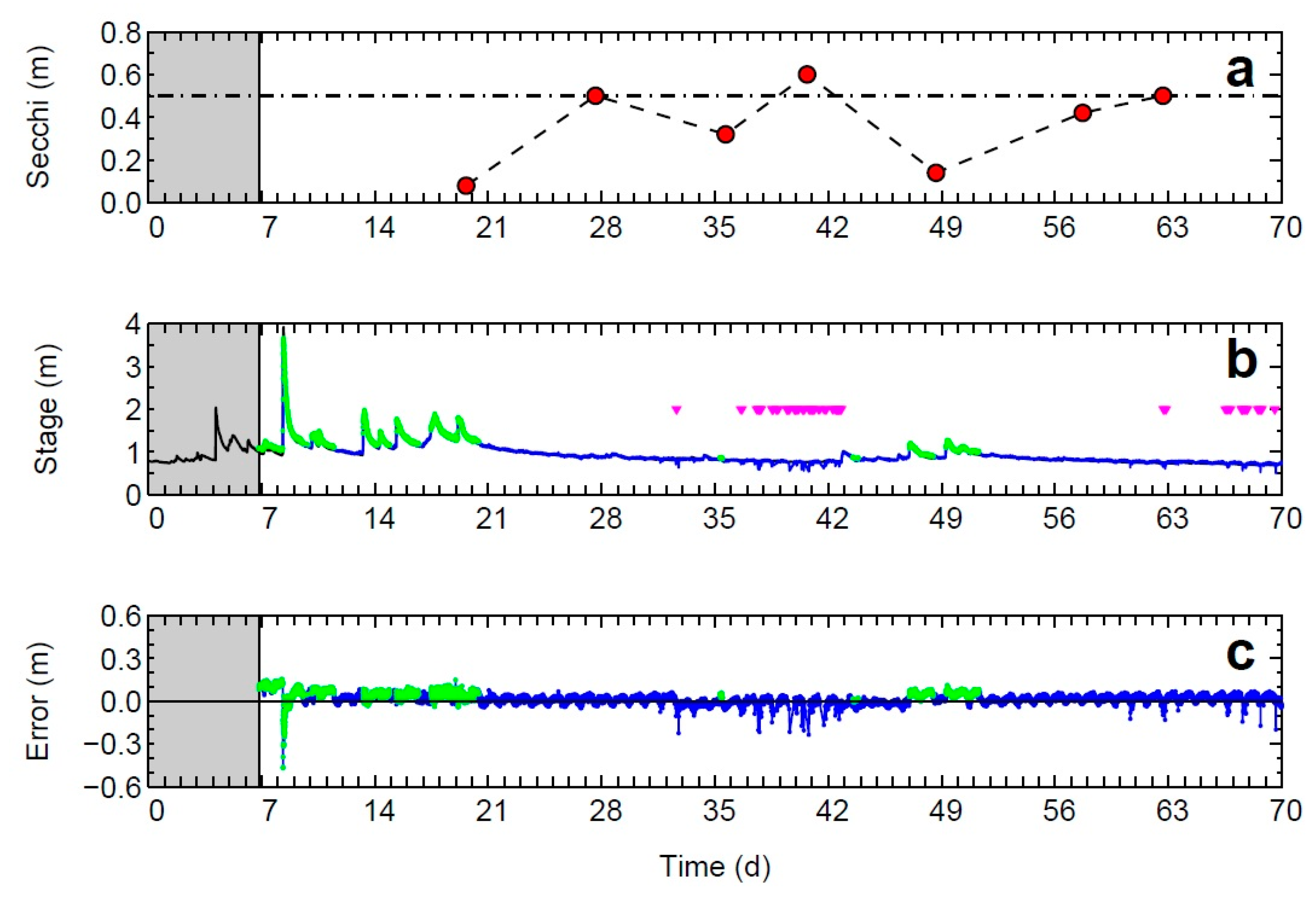
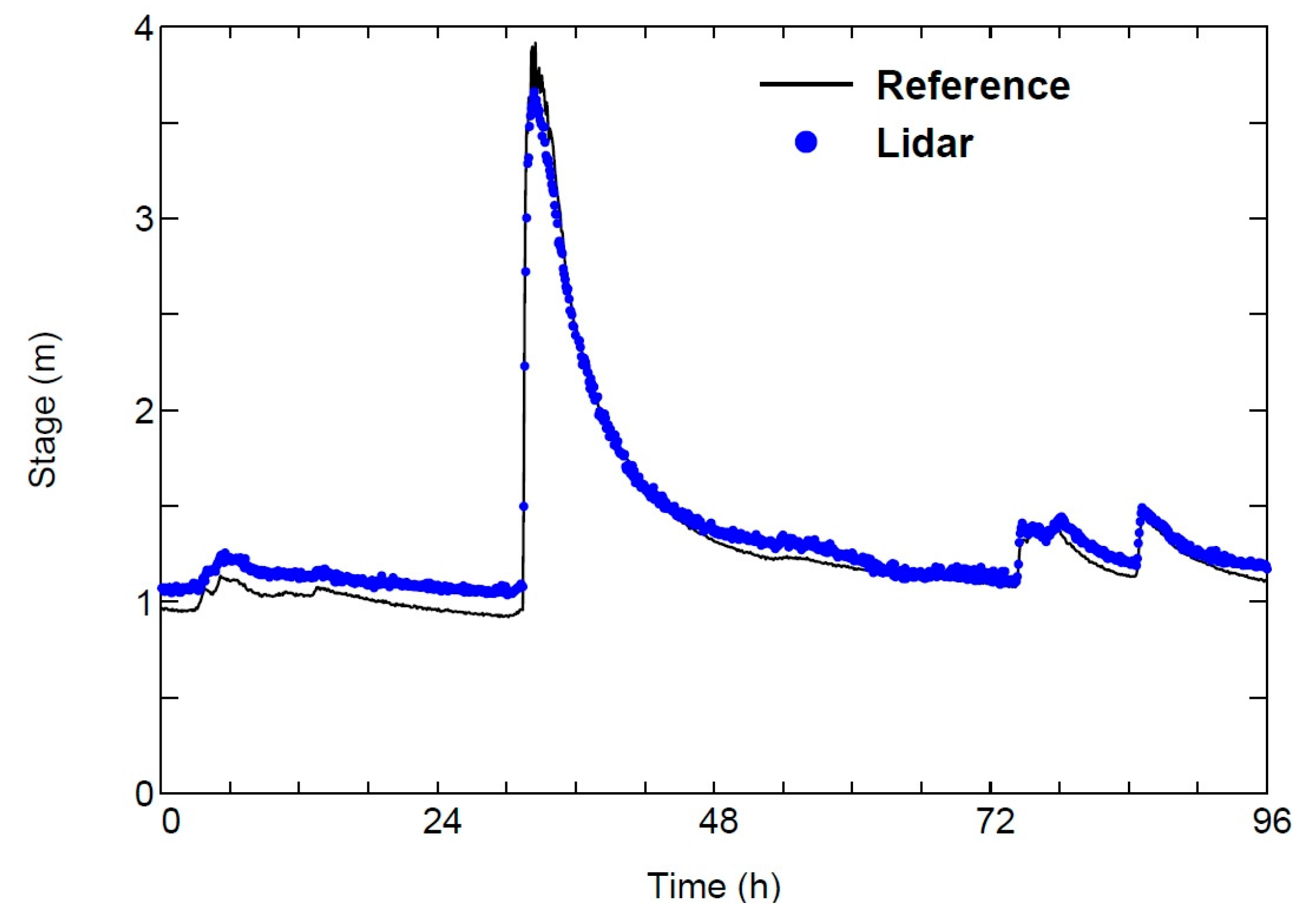
4.2. Stage Estimations

Ten small floods (sudden stage increase with a magnitude between 0.2 and 1.5 m) and one flash flood (stage increase of ≈2.5 m within 40 min) occurred during the monitoring campaign (nine weeks). The river was found to be extremely turbid, with a Secchi depth between 0.1 and 0.6 m (Figure 4a). Under these circumstances, the test Lidar was able to estimate stage data most of the time (Figure 4b), with no outlier when compared to the stage data obtained with the reference technique (Figure 4c). Globally (

Table 1. Performances of the inclined Lidar technique during the experiment in the Amacuzac River.

Numbers of attempts (every 5 min) to detect the water (sub) surface	Failed	3272 (15%)
	Succeeded	18,820 (85%)
Difference between the successful stage estimations by the inclined Lidar and the reference data (m)	Mean difference (b)	0.018
	Standard deviation (s)	0.034
	Symmetric coverage interval 1	±0.077
	Minimum difference	−0.470
	Maximum difference	0.153

¹ Computed as: $2\times \sqrt{b^2+s^2}$.

), 85% of the Lidar attempts to estimate stage data were successful, and these estimates were consistent within ±0.08 m (p = 0.95) with the reference data, which is close to what was expected from the preliminary uncertainty analysis (see Section 2.2).

In more detail, it was not at all difficult for the Lidar to detect the water (sub) surface when the Secchi depth was smaller than 0.5 m, which occurred most of the time, except during two periods of low water (see times ≈35 and 63 d in Figure 4a). In particular, the Lidar easily monitored the stage with a good temporal accuracy during the passing of the flash flood (Figure 5). It must be recognized that a rather large stage difference with reference data (≈0.5 m) was obtained at the peak discharge. However, this could be partly due to the fact that the Lidar was not pointing exactly at the bridge where the reference technique was installed but rather slightly upstream. In addition, a large tree trunk got stuck in front of the bridge during the flash flood and this may have slightly modified the hydraulic conditions where the reference technique was installed (the trunk was removed three weeks later).

It must be recognized that it became difficult for the test Lidar to detect the water (sub) surface during the two low-water periods when the water was slightly less turbid (Secchi depth larger than 0.5 m). On the one hand, some attempts to estimate stage data were unsuccessful (see the triangles at Figure 4b). And on the other hand, the estimated stage data were lower than usual (see Figure 4c at times between 35 and 42 days and at times between 63 and 70 days), which was probably because the Lidar laser beam penetrates deeper into the water when it is less turbid. Finally, small daily oscillation of the Lidar data (with an amplitude of ≈0.2 m) were obtained during periods with less turbid water: as discussed previously [16], this could be due to a natural phenomenon (such as a diurnal alternation between settlement and resuspension of mineral particles), although more studies are required to corroborate this hypothesis.

5. Concluding Remarks

5.1. Where Could an Inclined Lidar Be Used to Monitor Flash Floods?

It has been shown that the inclined Lidar technique can be used to monitor flash floods provided that the water is extremely turbid. According to this study and to a previous one [16], this would correspond to a Secchi depth smaller than ≈0.5 m. As an alternative, it can be checked that a red laser beam produces a Tyndall effect as it penetrates into water (as shown in Figure 2c).

The question now arises as to know a priori which catchments may be suitable for using the inclined Lidar technique to monitor flash floods. As a matter of fact, the instantaneous relationship between the water turbidity and the discharge in a river can be very complicated. Although it is traditionally considered that for a given river, the turbidity roughly tends to increase as a power function of the discharge rate [20], this does not necessarily mean that the turbidity will immediately increase at the beginning of any flood. Sometimes the turbidity begins to increase after a certain delay [21,22] and in this case, the inclined Lidar technique of course would not be very useful.

The monitoring of flash floods in intermittent rivers in arid areas is at least one case for which the inclined Lidar technique is likely to be suitable [23]. We also believe that the technique would be suitable for many others rivers since it is sensitive to small particles (clay or silt, from a granulometric point of view [16]): those which are at the bottom of a river bed or on the banks should be easily dragged and rapidly suspended at the beginning of a flash flood (e.g., [21]). However, will the amount of small suspended particles always be sufficient for an inclined Lidar to detect them? More studies are required to answer this question. Meanwhile, the knowledge of people who live near flooding rivers can be helpful: for instance, at the beginning of this study those responsible for the Amacuzac gauging station said that “the river always turns chocolate during a flood”.

5.2. What Is the Potential Interest of Detecting a Water (Sub) Surface with an Inclined Lidar?

As far as we know, this is the first evidence that an inclined Lidar can be used to monitor the stage of a river when it is flooding. If this works for other rivers that have problems with flash floods, the technique is attractive because it is easy to implement in a safe place (within less than two hours) and inexpensive (considering all the costs, including: acquisition, installation, and maintenance). In addition, it must be remembered that if an inclined Lidar detects suspended particles below the water surface, it can potentially determine their velocity relative to the Lidar line-of-sight (using the Doppler effect): an idea patented almost twenty years ago [24], but not yet officially tested (please, note that the setup considered in this study is different from that of conventional Laser Doppler Velocimetry (LDV), where the laser beam is focused with a lens on a small water volume). So, this study indirectly shows that a Lidar could potentially be used to monitor the subsurface water velocity during flash floods. Finally, it would be of interest to investigate whether the signal strength measured by a terrestrial inclined near-infrared Lidar can be used as a surrogate to monitor water turbidity (see Appendix B).

References

1. Jonkman, S.N. Global perspectives on loss of human life caused by floods. Nat. Hazards 2005, 34, 151–175. [Google Scholar] [CrossRef]
2. Borga, M.; Stoffel, M.; Marchi, L.; Marra, F.; Jakob, M. Hydrogeomorphic response to extreme rainfall in headwater systems: Flash floods and debris flows. J. Hydrol. 2014, 518, 194–205. [Google Scholar] [CrossRef]
3. Hill, C.; Verjee, F.; Barrett, C. Flash Flood Early Warning System Reference Guide; University Corporation for Atmospheric Research: Boulder, CO, USA, 2010. [Google Scholar]
4. Hall, J.; Arheimer, B.; Borga, M.; Brázdil, R.; Claps, P.; Kiss, A.; Kjeldsen, T.R.; Kriaučiuniene, J.; Kundzewicz, Z.W.; Lang, M.; et al. Understanding flood regime changes in Europe: A state of the art assessment. Hydrol. Earth Syst. Sci. 2014, 18, 2735–2772. [Google Scholar] [CrossRef] [Green Version]
5. Sauer, V.B.; Turnipseed, D.P. Stage Measurement at Gaging Stations; U.S. Geological Survey: Reston, VA, USA, 2010.
6. Tamari, S.; Sánchez, G.; Magos-Hernández, J.; López, E. Monitoreo del tirante en ríos: Prueba a medio plazo con sistemas de burbujeo y Radares. Tecnología y Ciencias del Agua 2016. in preparation. [Google Scholar]
7. Mishra, A.K.; Coulibaly, P. Developments in hydrometric network design: A review. Rev. Geophys. 2009, 47. [Google Scholar] [CrossRef]
8. Basha, E.; Rus, D. Design of early warning flood detection systems for developing countries. In Proceedings of the Information and Communication Technologies and Development (ICTD 2007), Bangalore, India, 15–16 December 2007; pp. 1–10.
9. Fritz, H.M.; Phillips, D.A.; Okayasu, A.; Shimozono, T.; Liu, H.; Mohammed, F.; Skanavis, V.; Synolakis, C.E.; Takahashi, T. The 2011 Japan tsunami current velocity measurements from survivor videos at Kesennuma Bay using Lidar. Geophys. Res. Lett. 2012, 39. [Google Scholar] [CrossRef]
10. Le Boursicaud, R.; Pénard, L.; Hauet, A.; Thollet, F.; Le Coz, J. Gauging extreme floods on YouTube: Application of LSPIV to home movies for the post-event determination of stream discharges. Hydrol. Process. 2016, 30, 90–105. [Google Scholar] [CrossRef]
11. Bechle, A.J.; Wu, C.H.; Liu, W.C.; Kimura, N. Development and application of an automated river-estuary discharge imaging system. J. Hydraul. Eng. 2012, 138, 327–339. [Google Scholar] [CrossRef]
12. Stumpf, A.; Augereau, E.; Delacourt, C.; Bonnier, J. Photogrammetric discharge monitoring of small tropical mountain rivers: A case study at Rivière des Pluies, Réunion Island. Water Resour. Res. 2016, 52, 4550–4570. [Google Scholar] [CrossRef]
13. Plant, W.J.; Keller, W.C.; Hayes, K. Measurement of river surface currents with coherent microwave systems. IEEE Trans. Geosci. Remote Sens. 2005, 43, 1242–1257. [Google Scholar] [CrossRef]
14. Welber, M.; Le Coz, J.; Laronne, J.B.; Zolezzi, G.; Zamler, D.; Dramais, G.; Hauet, A.; Salvaro, M. Field assessment of noncontact stream gauging using portable surface velocity Radars (SVR). Water Resour. Res. 2016, 52, 1108–1126. [Google Scholar] [CrossRef]
15. Tamari, S.; Garcia, F.; Arciniega-Ambrocio, J.I.; Porter, A. Laboratory and Field Testing of a Handheld Radar to Measure the Water Velocity at the Surface of Channels. Available online: http:// www.imta.gob.mx/biblioteca/libros_html/laboratory-field-testing/laboratory-field-testing.pdf (accessed on 12 October 2016).
16. Tamari, S.; Guerrero-Meza, V.; Rifad, Y.; Bravo-Inclán, L.; Sánchez-Chávez, J.J. Stage monitoring in turbid reservoirs with an inclined terrestrial near-infrared Lidar. Remote Sens. 2016. Acceptation or Rejection.. [Google Scholar]
17. JCGM. Evaluation of Measurement Data—Guide to the Expression of Uncertainty in Measurement (JCGM 100:2008); Working Group 1 of the Joint Committee for Guides in Metrology (JCGM/WG1): Paris, France, 2008. [Google Scholar]
18. Laser Technology Inc. True Sense S200 Series: User’s Manual, 7th ed.; Laser Technology Inc. (LTI): Centennial, CO, USA, 2014. [Google Scholar]
19. Davies-Colley, R.J.; Smith, D.G. Turbidity, suspended sediment, and water clarity: A review. JAWRA 2001, 37, 1085–1101. [Google Scholar]
20. Leopold, L.B.; Maddock, T., Jr. The Hydraulic Geometry of Stream Channels and Some Physiographic Implications; U.S. Geological Survey: Reston, VA, USA, 1953.
21. Lenzi, M.A.; Marchi, L. Suspended sediment load during floods in a small stream of the Dolomites (northeastern Italy). Catena 2000, 39, 267–282. [Google Scholar] [CrossRef]
22. Gao, P.; Nearing, M.A.; Commons, M. Suspended sediment transport at the instantaneous and event time scales in semiarid watersheds of southeastern Arizona, USA. Water Resour. Res. 2013, 49, 6857–6870. [Google Scholar] [CrossRef]
23. Cohen, H.; Laronne, J.B. High rates of sediment transport by flashfloods in the Southern Judean Desert, Israel. Hydrol. Process. 2005, 19, 1687–1702. [Google Scholar] [CrossRef]
24. Marsh, L.B.; Heckman, D.B. Open Channel Flowmeter Utilizing Surface Velocity and Lookdown Level Devices. U.S. Patent 5,811,688, 22 September 1998. [Google Scholar]
25. Palmer, S.C.J.; Pelevin, V.V.; Goncharenko, I.; Kovács, A.W.; Zlinszky, A.; Présing, M.; Horváth, H.; Nicolás-Perea, V.; Balzter, H.; Tóth, V.R. Ultraviolet fluorescence Lidar (UFL) as a measurement tool for water quality parameters in turbid lake conditions. Remote Sens. 2013, 5, 4405–4422. [Google Scholar] [CrossRef] [Green Version]
26. ISO. Hydrometry—Suspended Sediment in Streams and Canals—Determination of Concentration by Surrogate Techniques (ISO 11657:2014); International Organization for Standardization (ISO): Geneva, Switzerland, 2014. [Google Scholar]
Figure 1. Theoretical uncertainty of the inclined Lidar technique, given a simple (one-point) calibration. Equation 2 was applied to three Lidar incidence angles (θ) and with input uncertainties that can be easily achieved in practice: U(D) = 0.08 m and U(θ) = 0.01 rad (≈0.6°).
Remotesensing 08 00834 g001
Figure 2. Experiment at the Amacuzac River (Mexico): (a) monitoring system with an inclined Lidar (looking northeast); (b) close-up of the inclined Lidar (with a sun shield to prevent overheating); (c) Tyndall effect (arrow) observed with a red laser beam (pointer of an inclined handheld laser rangefinder, which was taking erroneous distance data in this case); (d) Secchi disk used to assess water transparency.
Remotesensing 08 00834 g002
Figure 3. Raw distance data measured by the tested Lidar during the experiment in the Amacuzac River. Each row corresponds to a different Lidar configuration: (a) “first pulse”; (b) “strongest pulse”; and (c) “last pulse”. Blue symbols show data associated with moderate signal strength (I = 3) and green symbols show data associated with a high signal strength (I = 4).
Remotesensing 08 00834 g003
Figure 4. Summary of the monitoring campaign in the Amacuzac River (Mexico): (a) water transparency; (b) stage data obtained with the reference (black line) and the proposed Lidar technique (blue line shows data associated with moderate signal strength and green line shows data associated with a high signal strength; the triangles represent periods during which the Lidar was unable to provide stage data for more than 15 min); (c) error of the proposed technique (i.e., stage estimates minus reference values). Day “0” corresponds to 12 September 2015. Grey areas correspond to the times before the Lidar installation.
Remotesensing 08 00834 g004
Figure 5. Details of the monitoring campaign showing a flash flood (20 September 2015).
Remotesensing 08 00834 g005