
The RUNE Experiment—A Database of Remote-Sensing Observations of Near-Shore Winds

 ,
,  , and
, and
Abstract
:
1. Introduction
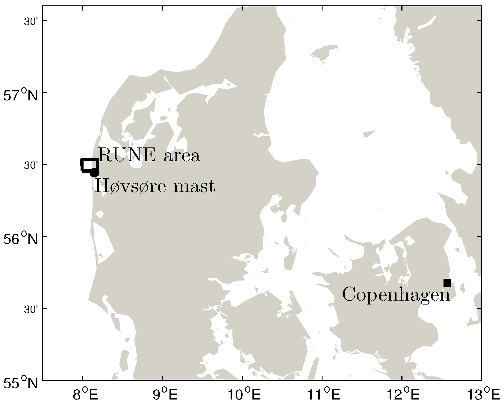
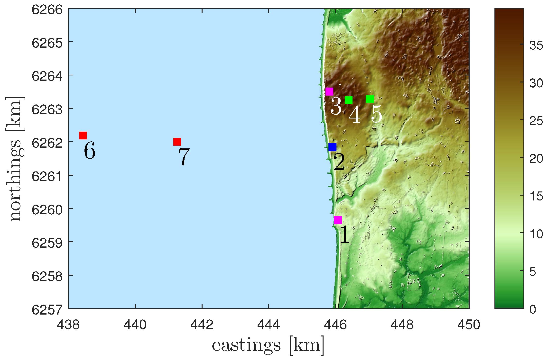
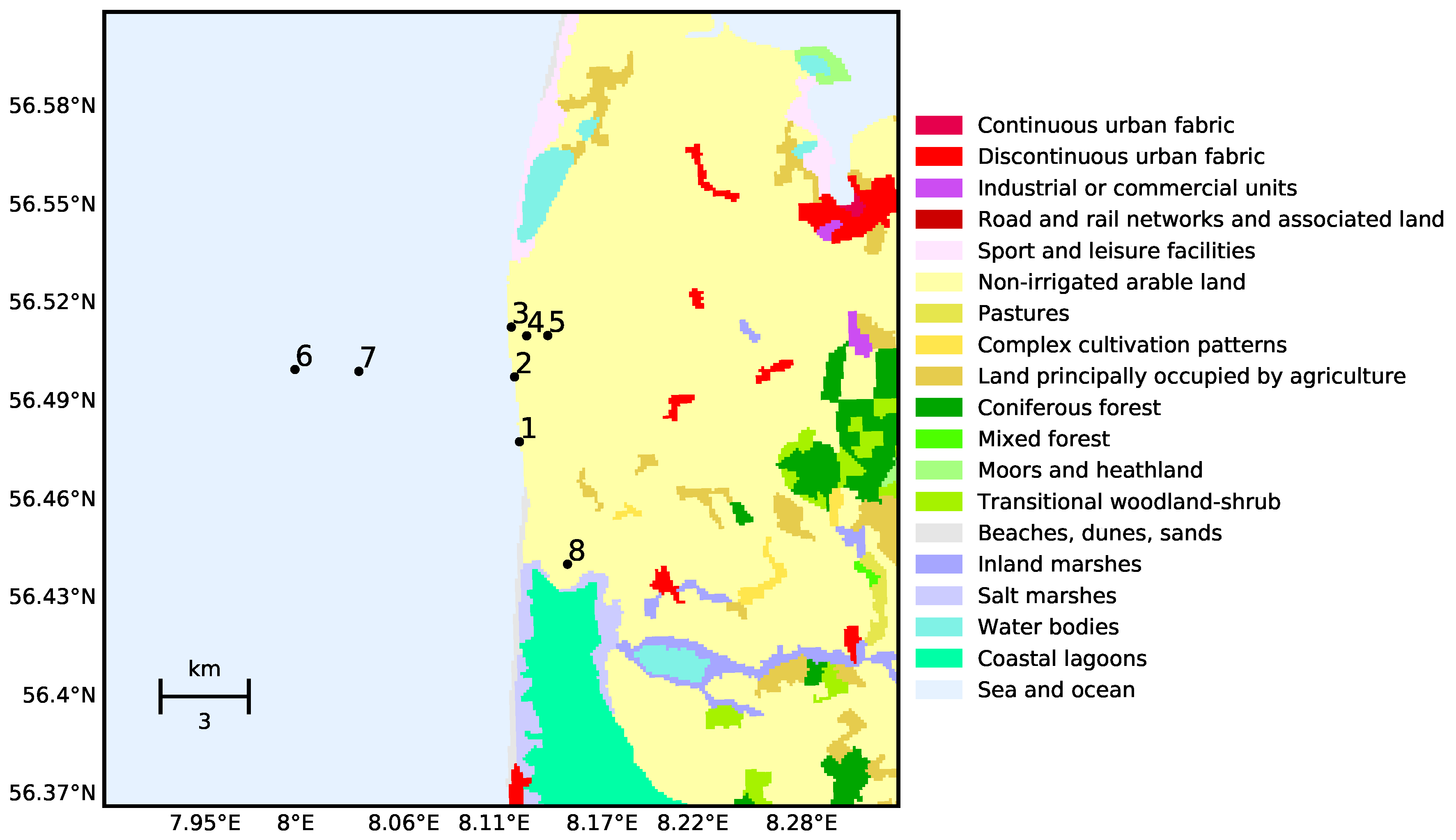
2. Site and Instruments
2.1. Timeline of the Campaign
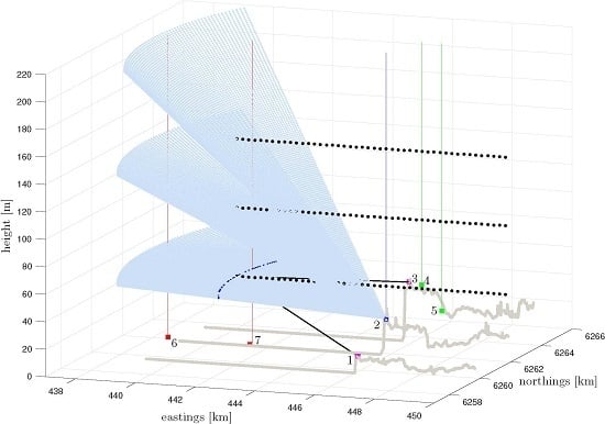
3. Setup of the Lidars
3.1. PPI Scans
3.2. Dual Setup
3.3. Virtual Mast
3.4. VAD Scans
4. Results
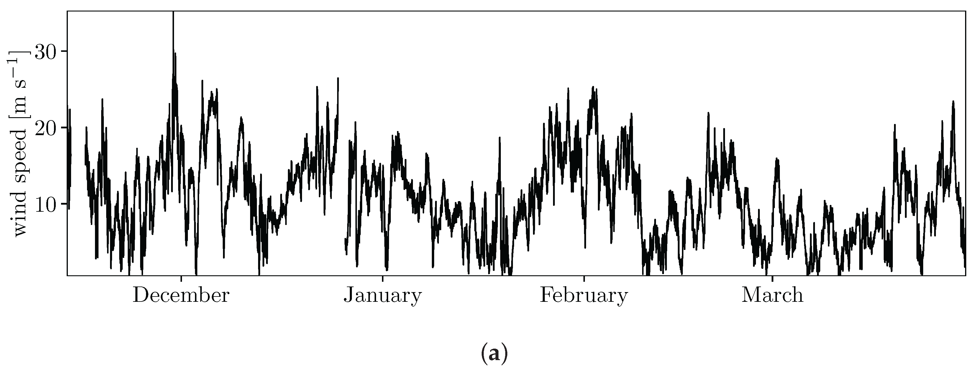
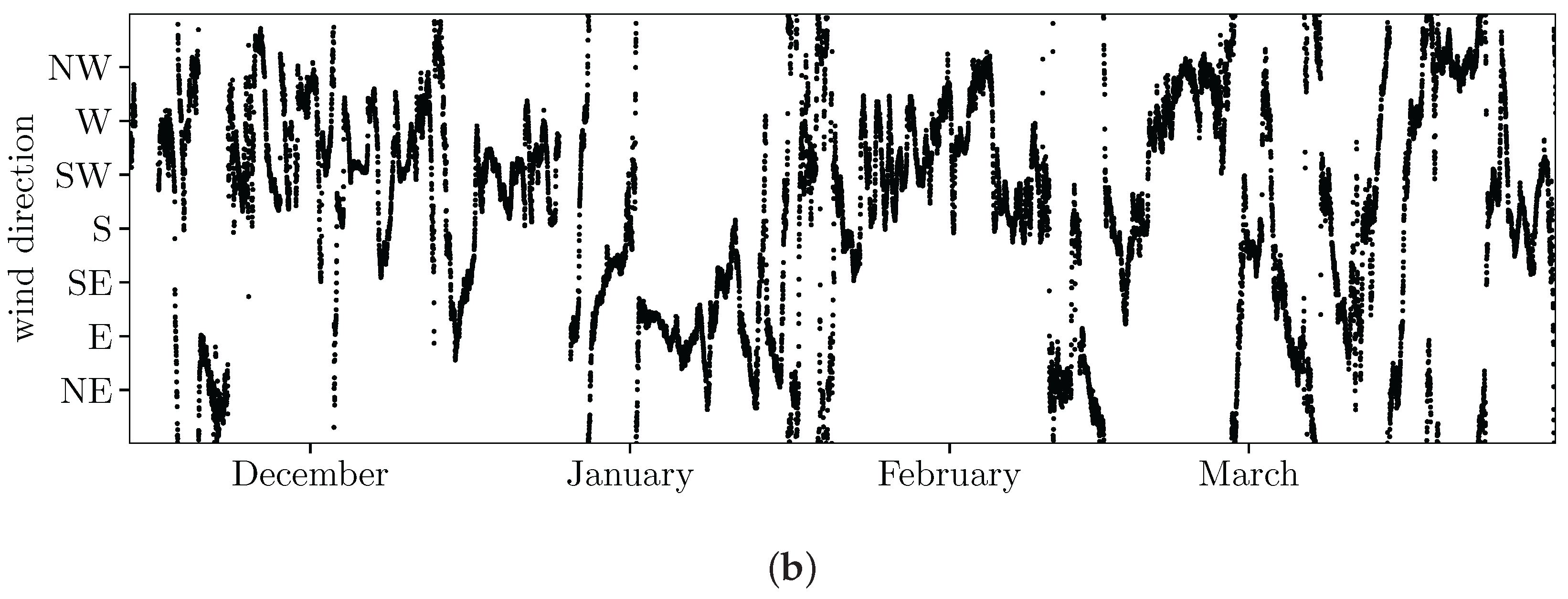
4.1. Wind Climate
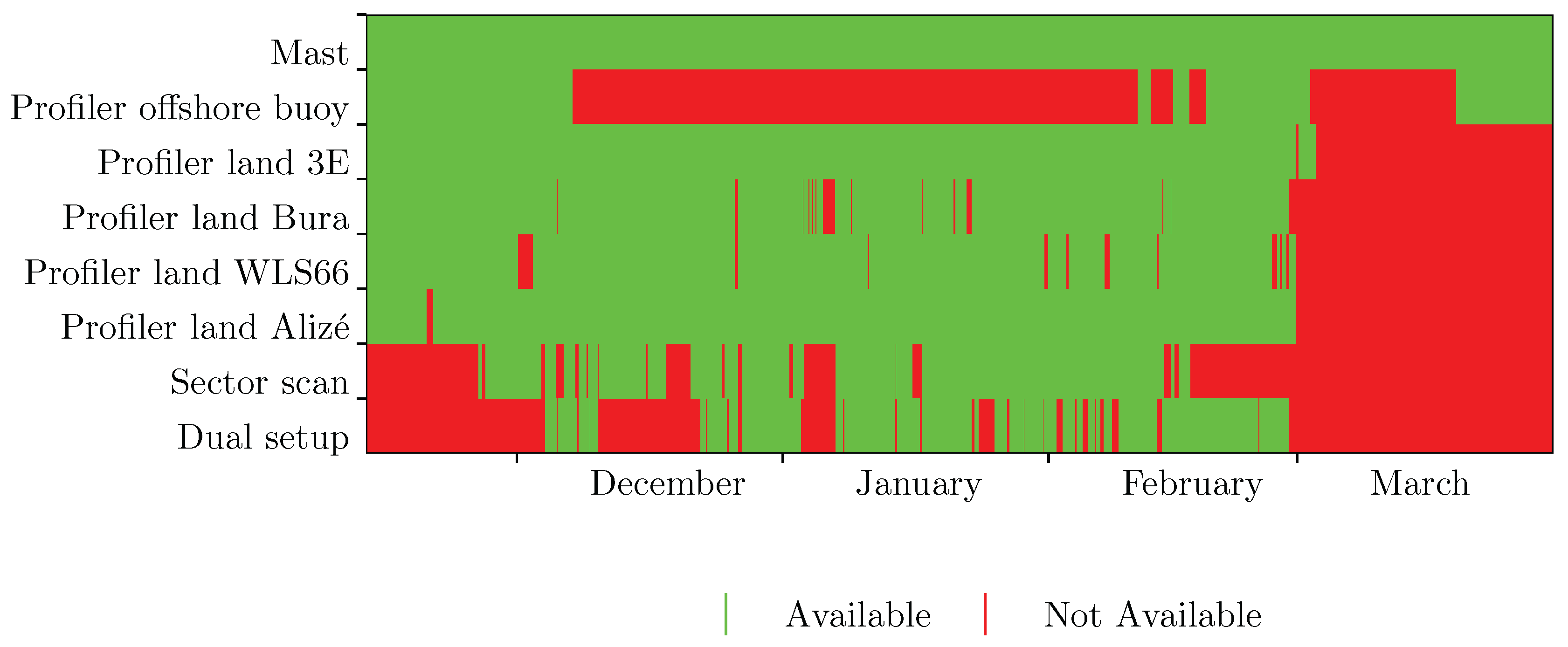
4.2. Actual Availability
4.3. Preliminary Intercomparisons
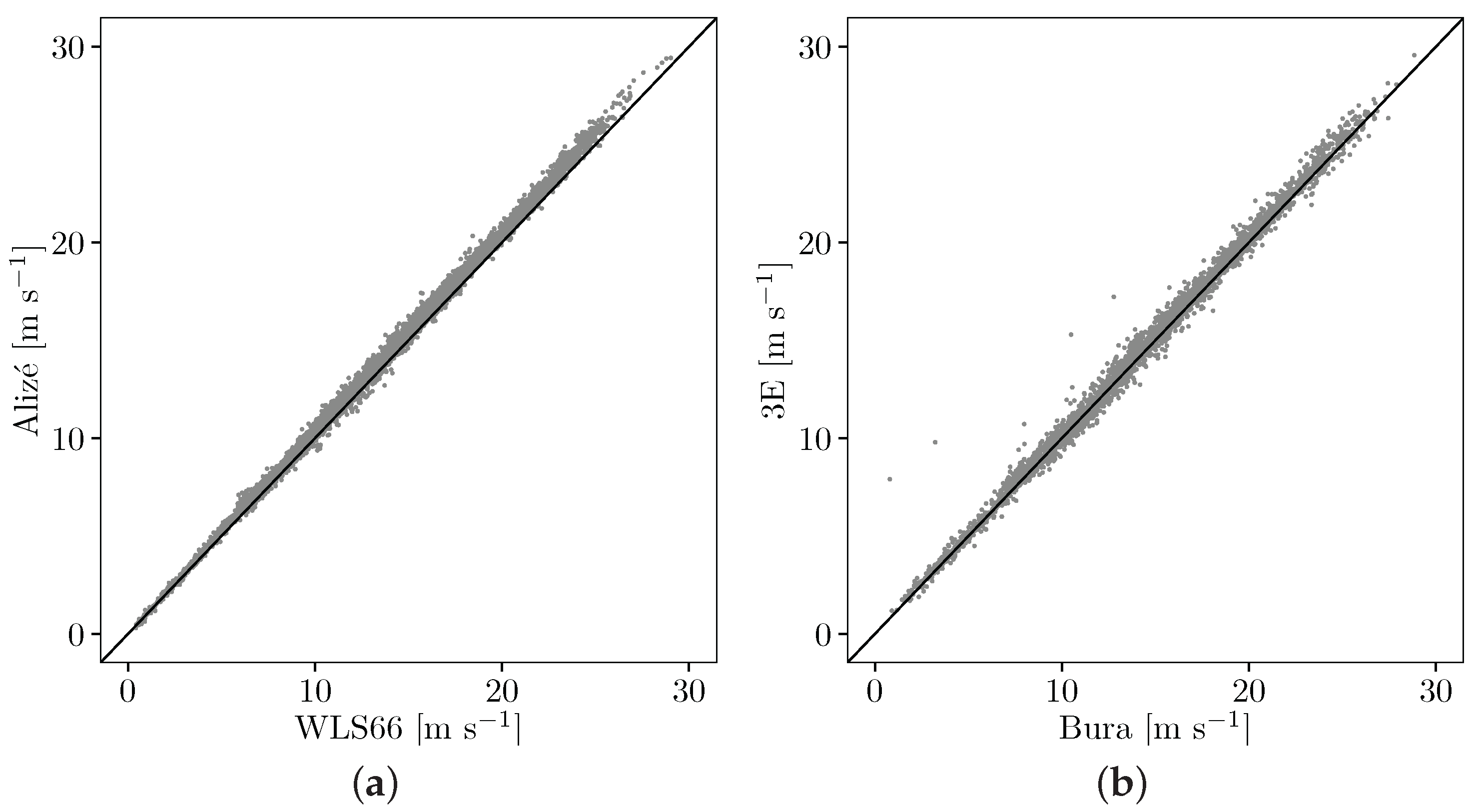
4.3.1. VAD Lidars
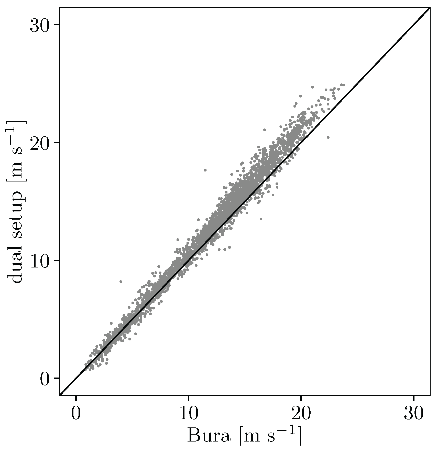
4.3.2. VAD and Dual Setup
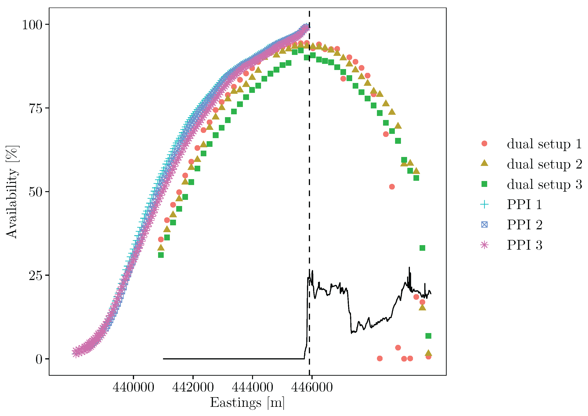
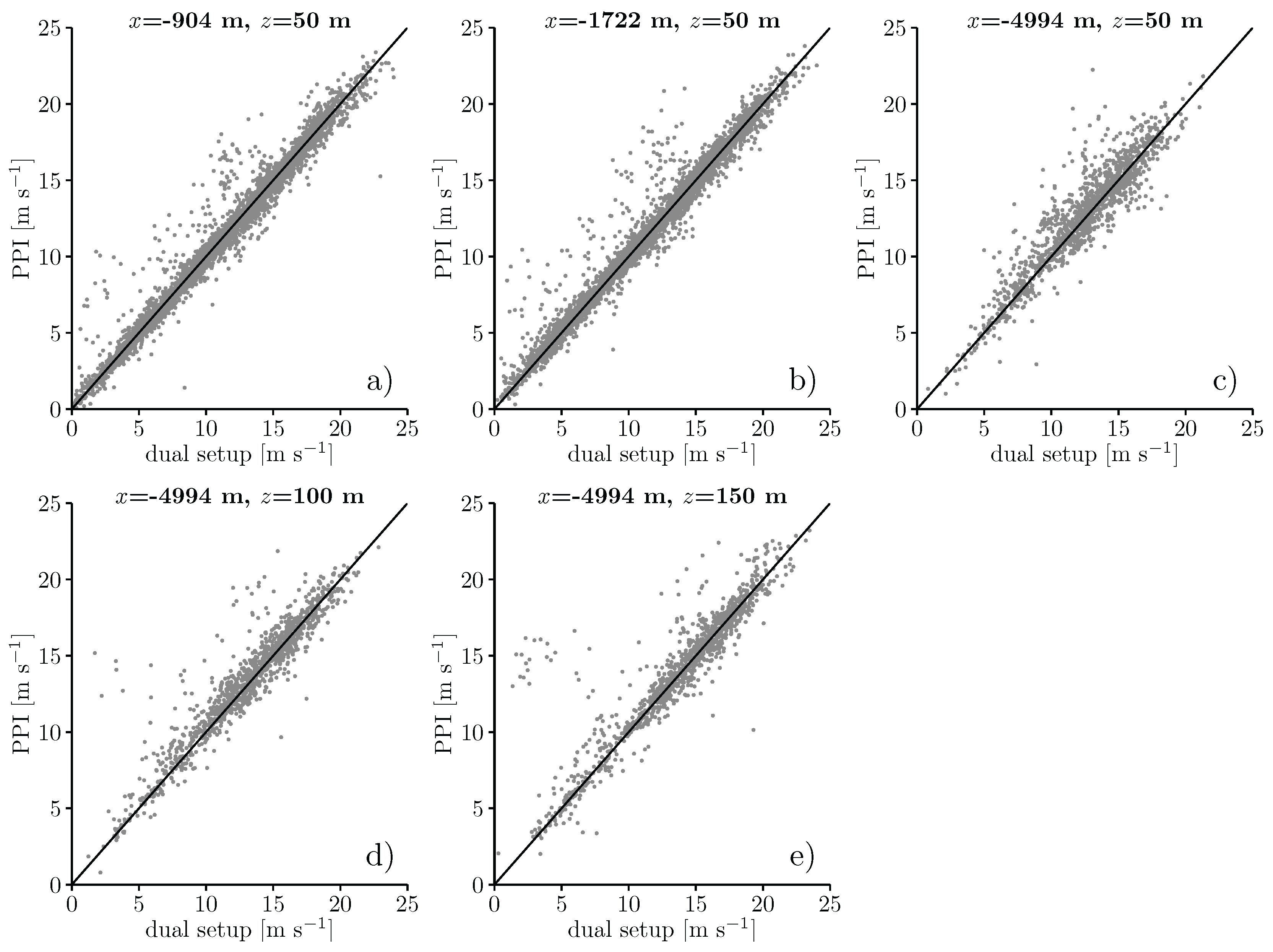
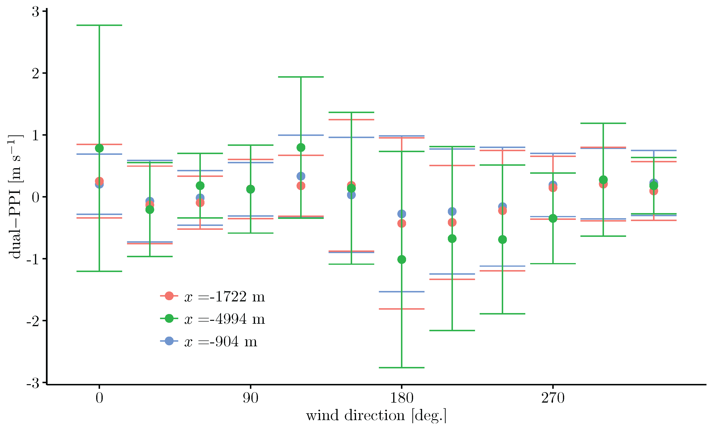
4.3.3. Dual Setup and PPIs
5. Conclusions
Acknowledgments
Author Contributions
Conflicts of Interest
References
- Floors, R.; Vincent, C.L.; Gryning, S.E.; Peña, A.; Batchvarova, E. The wind profile in the coastal boundary layer: Wind lidar measurements and numerical modelling. Bound.-Layer Meteorol. 2013, 147, 469–491. [Google Scholar] [CrossRef]
- Peña, A.; Gryning, S.E.; Hahmann, A. Observations of the atmospheric boundary layer height under marine upstream flow conditions at a coastal site. J. Geophys. Res. Atmos. 2013, 118, 1924–1940. [Google Scholar] [CrossRef]
- Mortensen, N.G.; Heathfield, D.N.; Myllerup, L.; Landberg, L.; Rathmann, O. Getting Started with WAsP 9; Technical Report Risø-I-2571(EN); Risø National Laboratory: Roskilde, Denmark, 2007. [Google Scholar]
- Frank, H.P.; Rathmann, O.; Mortensen, N.G.; Landberg, L. The Numerical Wind Atlas—The KAMM/WAsP Method; Technical Report Risø-R-1252(EN); Risø National Laboratory: Roskilde, Denmark, 2001. [Google Scholar]
- Landberg, L.; Myllerup, L.; Rathmann, O.; Petersen, E.L.; Jørgensen, B.H.; Badger, J.; Mortensen, N.G. Wind resource estimation—An overview. Wind Energy 2003, 6, 261–271. [Google Scholar] [CrossRef]
- Nunalee, C.G.; Basu, S. Mesoscale modeling of coastal low-level jets: Implications for offshore wind resource estimation. Wind Energy 2014, 17, 1199–1216. [Google Scholar] [CrossRef]
- Badger, J.; Frank, H.; Hahmann, A.N.; Giebel, G. Wind-climate estimation based on mesoscale and microscale modeling: Statistical-dynamical downscaling for wind energy applications. J. Appl. Meteorol. Climatol. 2014, 53, 1901–1919. [Google Scholar] [CrossRef]
- Smith, D.A.; Harris, M.; Coffey, A.S.; Mikkelsen, T.; Jørgensen, H.E.; Mann, J.; Danielian, R. Wind lidar evaluation at the Danish wind test site in Høvsøre. Wind Energy 2006, 9, 87–93. [Google Scholar] [CrossRef]
- Gottschall, J.; Courtney, M.S.; Wagner, R.; Jørgensen, H.E.; Antoniou, I. Lidar profilers in the context of wind energy—A verification procedure for traceable measurements. Wind Energy 2012, 15, 147–159. [Google Scholar] [CrossRef]
- Pauscher, L.; Vasiljevic, N.; Callies, D.; Lea, G.; Mann, J.; Klaas, T.; Hieronimus, J.; Gottschall, J.; Schwesig, A.; Kühn, M.; et al. An Inter-Comparison Study of Multi- and DBS Lidar Measurements in Complex Terrain. Remote Sens. 2016, 8, 782. [Google Scholar] [CrossRef]
- Vasiljević, N. A Time-Space Synchronization of Coherent Doppler Scanning Lidars for 3D Measurements of Wind Fields. Ph.D. Thesis, Danish Technical University, Roskilde, Denmark, 2014. [Google Scholar]
- Vasiljević, N.; Lea, G.; Courtney, M.; Cariou, J.P.; Mann, J.; Mikkelsen, T. Long-Range WindScanner System. Manuscript in Prep. Available online: http://dx.doi.org/10.20944/preprints201610.0017.v1 (accessed on 13 October 2016).
- Berg, J.; Vasiljevic, N.; Kelly, M.; Lea, G.; Courtney, M. Addressing spatial variability of surface-layer wind with long-range WindScanners. J. Atmos. Ocean. Technol. 2015, 32, 518–527. [Google Scholar] [CrossRef]
- Floors, R.; Lea, G.; Peña, A.; Karagali, I.; Ahsbahs, T. Report on RUNE’s Coastal Experiment and First Inter-Comparisons between Measurements Systems; Technical Report E-0115(EN); DTU Wind Energy: Roskilde, Denmark, 2016. [Google Scholar]
- Peña, A.; Floors, R.; Sathe, A.; Gryning, S.E.; Wagner, R.; Courtney, M.S.; Larsén, X.G.; Hahmann, A.N.; Hasager, C.B. Ten years of boundary-Layer and wind-power meteorology at Høvsøre, Denmark. Bound.-Layer Meteorol. 2016, 158, 1–26. [Google Scholar] [CrossRef]
- Courtney, M.; Simon, E. Deploying Scanning Lidars at Coastal Sites; Technical Report E-0110(EN); DTU Wind Energy: Roskilde, Denmark, 2016. [Google Scholar]
- Geostyrelsen. Available online: http://download.kortforsyningen.dk/content/dhm-2007overflade-16-m-grid (accessed on 21 June 2016).
- European Environment Agency. Available online: http://www.eea.europa.eu/data-and-maps/data/corine-land-cover-2006-raster-3{#}tab-metadata (accessed on 21 June 2016).
- Pindea, N.; Jorba, O.; Jorge, J.; Baldasano, J.M. Using NOAA-AVHRR and SPOT-VGT data to estimate surface parameters: Application to a mesoscale meteorological model. Int. J. Remote Sens. 2004, 25, 129–143. [Google Scholar] [CrossRef]
- Troen, I.; Petersen, E.L. European Wind Atlas; Risø National Laboratory: Roskilde, Denmark, 1989; p. 656. [Google Scholar]
- Floors, R.; Gryning, S.E.; Peña, A.; Batchvarova, E. Analysis of diabatic flow modification in the internal boundary layer. Meteorol. Z. 2011, 20, 649–659. [Google Scholar] [CrossRef]
- Liang, X. An integrating velocity—Azimuth process single-Doppler radar wind retrieval method. J. Atmos. Ocean. Technol. 2007, 24, 658–665. [Google Scholar] [CrossRef]
- Simon, E.I.; Courtney, M.S. A Comparison of Sector-Scan and Dual Doppler Wind Measurements at Høvsøre Test Station—One Lidar or Two? Technical Report DTU Wind Energy E-0112(EN); DTU Wind Energy: Roskilde, Denmark, 2016. [Google Scholar]
- Gottschall, J.; Wolken-Möhlmann, G.; Viergutz, T.; Lange, B. Results and conclusions of a floating-lidar offshore test. Energy Procedia 2014, 53, 156–161. [Google Scholar] [CrossRef]
- Mann, J.; Angelou, N.; Arnqvist, J.; Callies, D.; Cantero, E.; Chávez Arroyo, R.; Courtney, M.; Cuxart, J.; Dellwik, E.; Gottschall, J.; et al. Complex terrain experiments in the New European Wind Atlas. Philos. Trans. R. Soc. A 2016, in press. [Google Scholar]


| Position | Name | Type | Usage | Easting | Northing | Height |
|---|---|---|---|---|---|---|
| (m) | (m) | ASL (m) | ||||
| 1 | Koshava | WLS200S | Dual setup | 446,080.03 | 6,259,660.30 | 12.36 |
| 2 | Vara | WLS200S | PPI | 445,915.64 | 6,261,837.49 | 26.38 |
| 2 | Alizé | WLS70 | VAD | 445,915.64 | 6,261,837.49 | 26.38 |
| 2 | WLS66 | WLS7v1 | VAD | 445,915.64 | 6,261,837.49 | 26.38 |
| 3 | Sterenn | WLS200S | Dual setup | 445,823.66 | 6,263,507.90 | 42.97 |
| 4 | 3E | WLS7v1 | VAD | 446,379.30 | 6,263,251.46 | 43.18 |
| 5 | Bura | WLS7v1 | VAD | 447,040.74 | 6,263,273.41 | 24.93 |
| 6 | Lidar buoy | WLS7v2 | VAD | 438,441 | 6,262,178 | 0.00 |
| 7 | Lidar buoy | WLS7v2 | VAD | 440,616 | 6,262,085 | 0.00 |
| 8 | Høvsøre mast | Mast | 447,642 | 6,255,431 | 0.32 |
| Phase | System | Start Time Day/Month | End Time Day/Month | Scenario Type | Data (h) | Operational Availability (%) |
|---|---|---|---|---|---|---|
| 1 | Vara | 13/11 | 26/11 | PPI 1 | 251.5 | 79.25 |
| Sterenn | 17/11 | 27/11 | PPI 1 | 215.8 | 92.83 | |
| Koshava | 17/11 | 24/11 | PPI 1 | 145.9 | 91.99 | |
| 2 | Vara | 26/11 | 17/02 | PPI 3 | 1575.2 | 79.38 |
| Sterenn | 03/12 | 25/12 | dual v1 | 193.7 | 36.60 | |
| Koshava | 03/12 | 25/12 | dual v1 | 193.7 | 36.66 | |
| 3 | Sterenn | 25/12 | 17/02 | dual v2 | 1095.7 | 85.15 |
| Koshava | 25/12 | 17/02 | dual v2 | 1056.7 | 82.12 | |
| 4 | Vara | 17/02 | 29/02 | PPI 1 | 269.7 | 91.91 |
| Sterenn | 17/02 | 29/02 | RHI | 281.1 | 98.67 | |
| Koshava | 17/02 | 29/02 | RHI | 290.9 | 99.06 | |
| All | Alizé | 09/11 | 29/02 | VAD | 2625 | 97.52 |
| Bura | 12/11 | 28/02 | VAD | 2211 | 85.01 | |
| 3E | 01/11 | 02/03 | VAD | 2928.7 | 99.22 | |
| WLS66 | 01/11 | 29/02 | VAD | 2792.7 | 96.61 | |
| Lidar buoy 6 | 04/11 | 07/12 | VAD | 792 | 99.96 | |
| Lidar buoy 7 | 11/02 | 30/03 | VAD | 622.7 | 53.61 |
| Name | Range Gate Height ALL (m) |
| Alizé | 100, 150, 175, 200, 250, 300, 350, 400, 450, every 100 m from 500–1500 |
| Bura | 30, 35, 40, 50, 62, 75, 87, 100, 112, 125, 140, 155, 175, 200, 250, 300 |
| 3E | 40, 57, 70, 88, 107, 125, 150, 200, 250, 300 |
| WLS66 | 40, 50, 60, 74, 80, 90, 100, 110, 124, 150 |
| Lidar buoy | 40, 47, 59, 79, 97, 117, 134, 147, 172, 197, 209, 247 |
| Name | Range Gate Height ASL (m) |
| Virtual mast | 5, 28, 52, 75, 99, 122, 146, 169, 192, 217, 275, 298, 322, 345, 368, 392, |
| 415, 438, 461, 486, 520, 544, 568, 591, 615, 639, 662, 687, 710, 734, | |
| 757, 793, 816, 840, 864, 888 |
© 2016 by the authors; licensee MDPI, Basel, Switzerland. This article is an open access article distributed under the terms and conditions of the Creative Commons Attribution (CC-BY) license (http://creativecommons.org/licenses/by/4.0/).
Share and Cite
Floors, R.; Peña, A.; Lea, G.; Vasiljević, N.; Simon, E.; Courtney, M. The RUNE Experiment—A Database of Remote-Sensing Observations of Near-Shore Winds. Remote Sens. 2016, 8, 884. https://doi.org/10.3390/rs8110884
Floors R, Peña A, Lea G, Vasiljević N, Simon E, Courtney M. The RUNE Experiment—A Database of Remote-Sensing Observations of Near-Shore Winds. Remote Sensing. 2016; 8(11):884. https://doi.org/10.3390/rs8110884
Chicago/Turabian StyleFloors, Rogier, Alfredo Peña, Guillaume Lea, Nikola Vasiljević, Elliot Simon, and Michael Courtney. 2016. "The RUNE Experiment—A Database of Remote-Sensing Observations of Near-Shore Winds" Remote Sensing 8, no. 11: 884. https://doi.org/10.3390/rs8110884
APA StyleFloors, R., Peña, A., Lea, G., Vasiljević, N., Simon, E., & Courtney, M. (2016). The RUNE Experiment—A Database of Remote-Sensing Observations of Near-Shore Winds. Remote Sensing, 8(11), 884. https://doi.org/10.3390/rs8110884