A Methodology for the Reconstruction of 2D Horizontal Wind Fields of Wind Turbine Wakes Based on Dual-Doppler Lidar Measurements

Abstract

Dual-Doppler lidar is a powerful remote sensing technique that can accurately measure horizontal wind speeds and enable the reconstruction of two-dimensional wind fields based on measurements from two separate lidars. Previous research has provided a framework of dual-Doppler algorithms for processing both radar and lidar measurements, but their application to wake measurements has not been addressed in detail yet. The objective of this paper is to reconstruct two-dimensional wind fields of wind turbine wakes and assess the performance of dual-Doppler lidar scanning strategies, using the newly developed Multiple-Lidar Wind Field Evaluation Algorithm (MuLiWEA). This processes non-synchronous dual-Doppler lidar measurements and solves the horizontal wind field with a set of linear equations, also considering the mass continuity equation. MuLiWEA was applied on simulated measurements of a simulated wind turbine wake, with two typical dual-Doppler lidar measurement scenarios. The results showed inaccuracies caused by the inhomogeneous spatial distribution of the measurements in all directions, related to the ground-based scanning of a wind field at wind turbine hub height. Additionally, MuLiWEA was applied on a real dual-Doppler lidar measurement scenario in the German offshore wind farm “alpha ventus”. It was concluded that the performance of both simulated and real lidar measurement scenarios in combination with MuLiWEA is promising. Although the accuracy of the reconstructed wind fields is compromised by the practical limitations of an offshore dual-Doppler lidar measurement setup, the performance shows sufficient accuracy to serve as a basis for 10 min average steady wake model validation.

1. Introduction

Establishing sophisticated methods for measurement and analysis of wake effects [1] in wind farms is relevant nowadays, since large offshore wind farms can experience wake losses of between 10% and 20% of their annual energy production [2]. By acquiring more knowledge about wakes, their negative impacts on large wind farms can be mitigated e.g., by improving wind farm layout design [3] or by applying innovative wind farm control strategies [4].

The high potential of lidars [5,6] has been demonstrated for different wind energy applications in general [7,8,9], and for measuring wakes in particular [10,11]. Coherent Doppler lidars [12,13] measure the Doppler shift of frequency between the emitted and backscattered laser light, which is converted to a radial velocity estimate. Long-range pulsed lidars [14] offer the possibility to scan over areas of several square kilometers within a few minutes. Käsler et al. [15] were among the first to execute wake measurements of a turbine with such a lidar. Aitken et al. [16] retrieved wake characteristics by using one long-range lidar and fitting measurements to Gaussian-shaped wake profiles. Banta et al. [17] proposed a way to execute volumetric measurements with a single lidar. Iungo et al. [18] used dual-Doppler lidar to scan a vertical plane through a wind turbine wake.

Considerable uncertainties can affect the horizontal wind vector reconstructed from measurements performed with a single lidar. This aspect is even more relevant in the wake of a wind turbine where the wind field is heterogeneous. Using a single representative wind direction—e.g., provided by a nearby wind vane—to evaluate the horizontal wind vector derived from the radial wind velocity measured over a large area within a wind farm, could introduce uncertainties due to the local variability of the wind direction. Moreover, the propagation of all uncertainties affecting the reconstruction of the horizontal wind vector tends to grow infinitely when the lidar measures perpendicular to the wind direction. This limits the possibility to perform reliable measurements of a wind turbine wake.

Advanced dual-Doppler lidar applications could overcome these problems by using multiple lidars to scan over the same area of interest from different locations, optionally considering the continuity equation as well. We are subsequently referring to dual-Doppler lidar as methods for performing and processing measurements from different Plan Position Indicator (PPI) scans of two long-range pulsed scanning lidars. The PPI scan is characterised by a fixed elevation angle and a varying azimuth angle. When several elevation angles are considered and a full-volume of dual-Doppler lidar measurements is available, it is possible to evaluate 2D or 3D wind fields on a predefined grid by means of algorithms such as the Multiple-Doppler Synthesis and Continuity Adjustment Technique (MUSCAT) by [19]. This was originally developed for airborne radar [20] and was evaluated mainly for the study of meteorological steady wind fields in which the measurement domain was in the order of 1000 km² [21]. Drechsel et al. [22] demonstrated the feasibility of the application of MUSCAT to ground-based dual-Doppler lidar measurements. In the latter study, a full-volume scan defined by a 360° sector at 10 different elevation angles lasted about 20 min. This points out that the small time and length scale dynamics of wind turbine wakes and the time needed for a full-volume scan cycle could conflict when applying dual-Doppler lidar to wake measurements. On the contrary, with a full-volume scan cycle of about 1 min, the application of two Ka-band radars [23] could enable the study of the dynamical behaviour of wakes in a wind farm.

Although the application of the aforementioned dual-Doppler analysis algorithms in combination with the state-of-the-art dual-Doppler lidar scanning techniques was demonstrated before, the application to wind turbine wakes has not been analysed thoroughly yet. In this paper, we propose a simple wind field reconstruction methodology similar to MUSCAT, which we call Multiple-Lidar Wind Field Evaluation Algorithm (MuLiWEA). This implementation is meant to reduce the uncertainty in the evaluation of the horizontal wind speeds, especially for situations in which the inclination between the wind direction and the line-of-sight direction of the radial wind speed measurement of one lidar is close to 90°.

The application of MuLiWEA does not require a set of fully synchronised dual-Doppler lidar measurements because it performs grid interpolation. This feature offers the possibility to use measurements from scanning scenarios with low complexity and fast area coverage.

We applied MuLiWEA to dual-Doppler lidar measurements simulated in the wake of a wind turbine, considering a series of different scanning scenarios, and compared the reconstructed wind fields to the simulated ones. Additionally, we analysed a test case based on real dual-Doppler lidar measurements offshore.

2. Methodology

The MuLiWEA algorithm is based on the following assumptions:

• The vertical wind speed component w is neglected because the elevation angles of the PPI scans are commonly small, and, therefore, it is difficult to estimate this component accurately from the measured line-of-sight velocity. This assumption limits the application of MuLiWEA to horizontal flows only, i.e., it might not be accurate in complex terrain sites, in convective atmosphere conditions, or in the near wake of a wind turbine.
• As a consequence of the previous assumption, no vertical transport of mass is considered in the continuity equation, which is therefore applied in its two-dimensional form.
• The flow is assumed to be stationary for the required time resolution because it generally takes a few minutes for the lidar scans to cover an area of interest, and it is useful to average a number of subsequent PPI scans to improve the data quality.
• The flow is assumed to be incompressible.

The measured line-of-sight velocity $v_{LOS}$ is expressed in the Cartesian wind speed components in the x- and y-direction, namely u and v, respectively, by Equation (1):

$${\alpha }_{k}u+{\beta }_{k}v=v_{LO{S}_k},$$

(1)

with $\alpha =sin\left(\chi \right)cos\left(\delta \right)$ and $\beta =cos\left(\chi \right)cos\left(\delta \right)$.

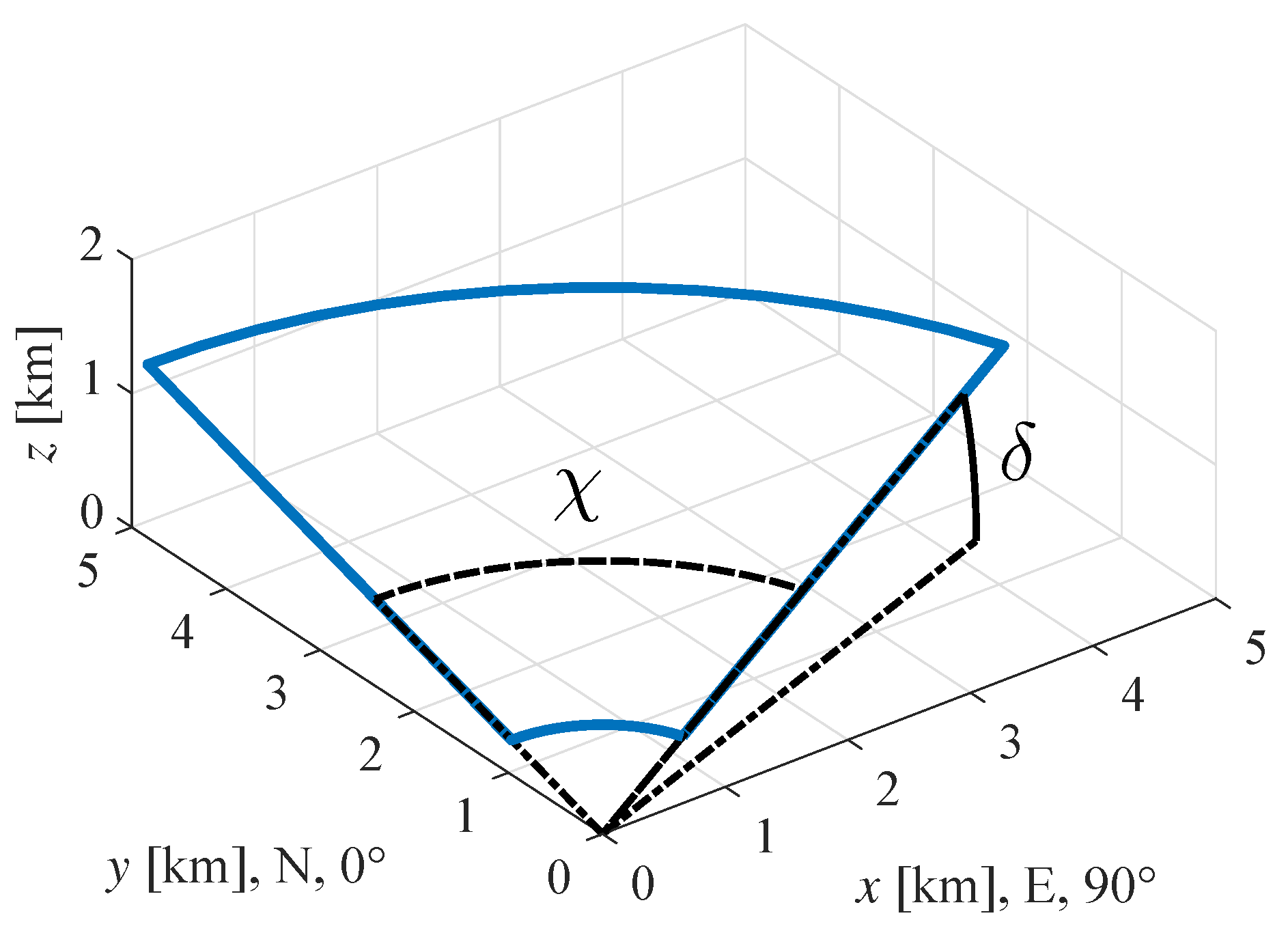
Note that Equation (1) already incorporates that $w=0$. The line-of-sight direction at a single measurement point k is defined by the azimuth angle χ and elevation angle δ of a lidar scanning beam (see Figure 1). The azimuth angle is expressed in the geographical reference system, i.e., $\chi =0°$ is directed to the North and increases clockwise. Since the angles are a known input with a certain pointing accuracy, the two remaining unknowns in Equation (1) are u and v. To solve for these two wind speed components, at least two linearly independent $v_{LOS}$ measurements are needed. Instead of fully synchronised measurements of two lidars at a single point in space at the same time (e.g., [18]), a concept to reconstruct 2D wind vector information from a larger set of PPI measurements from two lidars is used. In the worst case, the measurements are neither synchronised in time nor space. 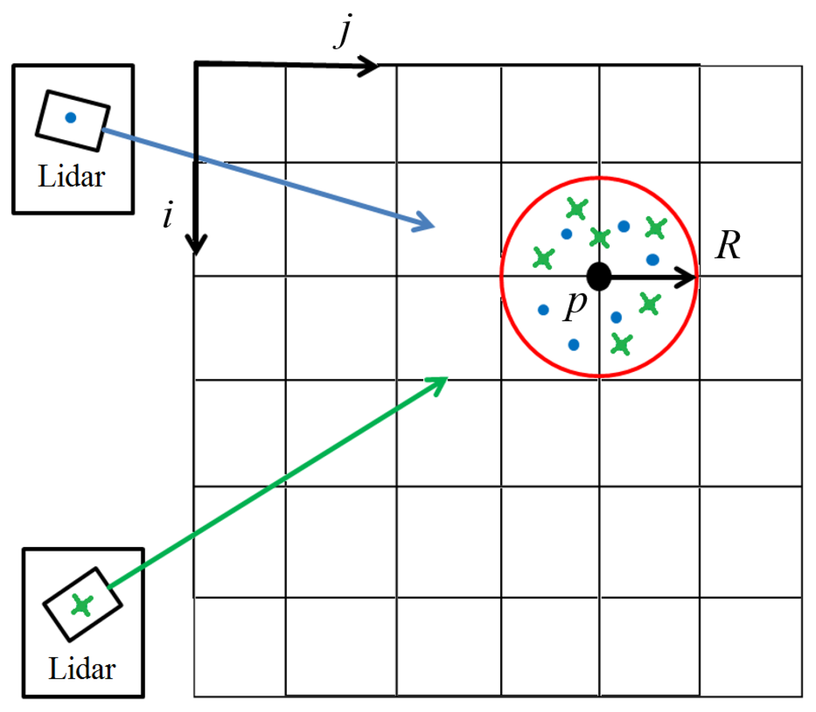Therefore, the method has to analyse samples of K measurements from the two lidars around each grid point p (see Figure 2) over a longer time period of e.g., ten minutes. Measurements in the near vicinity of a grid point rather than exactly at a grid point have to be used and measurements at different heights above ground have to be combined. A suitable protocol for measurement point selection is found in the form of the Quad-Doppler wind synthesis, a step of the Extended Overdetermined dual-Doppler Formalism (EODD) [20], later also used by Newsom et al. [24]. The reconstruction of a wind field can be divided into five sequential steps:

• A temporal and spatial domain is defined. To ensure that an area of interest is covered with at least one PPI scan per lidar, and possibly multiple overlapping scans to enhance averaging, a time resolution of ten minutes is chosen. A Cartesian grid is generated on the area of interest covered by the overlapping PPI scans. The assumption of stationarity posed before is considered to be reasonable for this time scale.
• For each grid point p, the measurement set K that is located within its surrounding circle with radius R, i.e., the radius of influence, is used to compute the local wind vector. The measurement set K contains contributions from all lidars (see Figure 2). Different lidars do not necessarily have to contribute an equal number of measurements for the same grid point.
• For each grid point p, a linear system based on Equation (1) can be established , which considers all measurements $k=1,...,K$ per circle with radius R [20]:

  $$\begin{array}{c}{\left[\begin{array}{cc}{\sum }_{k=1}^K\left({\alpha }_k^2{w}_k\right)& {\sum }_{k=1}^K\left({\alpha }_k{\beta }_k{w}_k\right)\\ {\sum }_{k=1}^K\left({\alpha }_k{\beta }_k{w}_k\right)& {\sum }_{k=1}^K\left({\beta }_k^2{w}_k\right)\end{array}\right]}_p{\left[\begin{array}{c}u\\ v\end{array}\right]}_p\hfill \\ ={\left[\begin{array}{c}{\sum }_{k=1}^K\left({\alpha }_k{w}_k{v}_{LO{S}_k}\right)\\ {\sum }_{k=1}^K\left({\beta }_k{w}_k{v}_{LO{S}_k}\right)\end{array}\right]}_{p,}\hfill \end{array}$$

  (2)

  in which $w_k$ is a weighting parameter, expressed as:

  $$w_k=\frac{R^2-r_k^2}{R^2+r_k^2}·\frac{K}{K_{l_k}L},$$

  (3)

  where $r_k$ is the distance between each measurement k to the grid point p, $K_{l_k}$ is the number of measurements contributed by the lidar l which corresponds to measurement k and L is the total count of contributing lidars.
  Different weighting functions have been used by other researchers for similar purposes [25,26], including the range gate weighting function of pulsed lidars [27]. The Cressman weighting procedure [25] was validated by comparison with sonic anemometer measurements by Newsom et al. [28]. In Equation (3), the first fraction resembles this Cressman weight, which is a parabolic function that assigns measurements a weight based on their distance $r_k$ to a grid point p inside the circle with radius of influence R. The second fraction is the lidar weight assigned to each single measurement k, which equalises the contributions from the lidars to the grid point. An additional weight considering the accuracy of each line-of-sight measurement, e.g., based on Carrier-to-Noise-Ratio (CNR), could also be included, but this is not addressed in this paper.
• For a grid of size m-by-n, there will be a number of $mn$ grid points p. Instead of solving Equation (2) for each grid point p, a sparse $2mn$-by-$2mn$ matrix $\mathbf{A}$ is defined. Each of the four elements inside the matrix in Equation (2) will form a diagonal with length $mn$ on the corresponding quadrant of the newly defined sparse matrix $\mathbf{A}$. Now, the larger set of linear equations is defined:

  $$\mathbf{A}\mathbf{x}=\mathbf{b},$$

  (4)

  with:

  $$\mathbf{x}=\left[\begin{array}{c}{u}_1\\ ⋮\\ ⋮\\ u_{mn}\\ v_1\\ ⋮\\ ⋮\\ v_{mn}\end{array}\right],\mathbf{b}=\left[\begin{array}{c}{\sum }_{k=1}^{K_1}{\left({\alpha }_k{w}_k{v}_{LO{S}_k}\right)}_1\\ ⋮\\ ⋮\\ {\sum }_{k=1}^{K_{mn}}{\left({\alpha }_k{w}_k{v}_{LO{S}_k}\right)}_{mn}\\ {\sum }_{k=1}^{K_1}{\left({\beta }_k{w}_k{v}_{LO{S}_k}\right)}_1\\ ⋮\\ ⋮\\ {\sum }_{k=1}^{K_{mn}}{\left({\beta }_k{w}_k{v}_{LO{S}_k}\right)}_{mn}\end{array}\right].$$

  (5)
• The continuity adjustment is included in the linear system in the form of additional rows, in order to establish an over-determined linear system. This provides a more robust system in case $\mathbf{A}$ is ill-defined, which could occur e.g., when there are local scarcities in the measurements or when a part of the line-of-sight measurements is linearly dependent. The two-dimensional continuity equation for incompressible flow can be written in differential form as:

  $$\frac{\partial u}{\partial x}+\frac{\partial v}{\partial y}=0.$$

  (6)
  For inclusion in the system, a numerical approximation of the continuity equation is necessary. Where applicable, the central difference scheme is used for expressing the partial differentials. At the grid boundaries, either upward or downward difference schemes [29] are needed due to a lack of neighboring points. By adding the continuity adjustment to $\mathbf{A}$, a new system with the $3mn$-by-$2mn$ matrix ${\mathbf{A}}_{\mathbf{C}}$ is created. There are still $2mn$ unknown variables, leaving the vector $\mathbf{x}$ unaffected. The vector ${\mathbf{b}}_{\mathbf{C}}$ is generated by extending $\mathbf{b}$ with $mn$ zeros. The final linear system,

  $${\mathbf{A}}_{\mathbf{C}}\mathbf{x}={\mathbf{b}}_{\mathbf{C}},$$

  (7)

  is an over-determined linear system, which is solved by minimising its squared residuals.

3. Application and Validation of MuLiWEA

3.1. Simulated Dual-Doppler Lidar Measurement Scenarios

To test MuLiWEA, different lidar measurement scenarios were simulated considering a weighted average of the line-of-sight velocity over the considered sample volume. The sample volume was defined along a linear coordinate s, which represents the line-of-sight distance from the lidar to the target point. We used a range gate length corresponding to a spatial extension $\Delta p$ of 36 m and a Gaussian laser pulse with intensity $I_p$, characterised by a Full Width Half Maximum $\Delta r$ of 30 m [14]:

$$I_p\left(s\right)=\frac{1}{\sqrt{\pi }\Delta r}{e}^{\left(-\frac{s^2}{\Delta r^2}\right)}.$$

(8)

The estimated line-of-sight velocity is then ${\widehat{v}}_{LOS}\left(s\right)=\frac{1}{\Delta p}{\int }_{\frac{-\Delta p}{2}}^{\frac{\Delta p}{2}}{v}_p\left(s\right)ds$, where $v_p\left(s\right)={\int }_{-k_p\frac{\Delta r}{2}}^{k_p\frac{\Delta r}{2}}{v}_{r^{\prime }}\left(s^{\prime }-s\right)I\left(s^{\prime }-s\right)d{s}^{\prime }$ with $I=\frac{I_p\left(s\right)}{{\int }_{-\infty }^{+\infty }{I}_p\left(s\right)}$ and $k_p=2.56$, where the primes denote the variable of integration along the line-of-sight distance s.

We simulated lidar measurements in the wake of a wind turbine with a rotor diameter of $D=62$ m and a hub height of $h_h=61$ m. To run the simulations, an unsteady wind field is calculated with the Parallelised Large-Eddy Simulation (LES) Model (PALM) [30]. The actuator line (ACL) approach [31] is included to simulate the wind turbine. For this experiment, a ten minute wind field is generated on a 4 m resolved grid with a temporal resolution of 0.4 s. The boundary conditions were chosen in order to simulate a neutral atmosphere (corresponding to a logarithmic vertical wind profile with roughness length $z_0=0.05$ m and a friction velocity $u_{*}=0.5$ m·s${}^{-1}$), an average inflow wind speed at hub height of 9 m·s${}^{-1}$, a wind direction of 270° (West) and a turbulence intensity $TI$ of 8% at hub height. In the lidar simulation used for testing MuLiWEA, the position of the laser beam was updated every 0.4 s. Within each range gate, fifteen equally spaced points of the corresponding sample volume were interpolated from the wind field. Finally, ${\widehat{v}}_{LOS}$ was evaluated numerically.

The validation procedure considers four different simulated lidar locations, two different PPI measurement scenarios and the effect of either enabling or disabling the continuity adjustment. The two following different PPI measurement scenarios were simulated and evaluated:

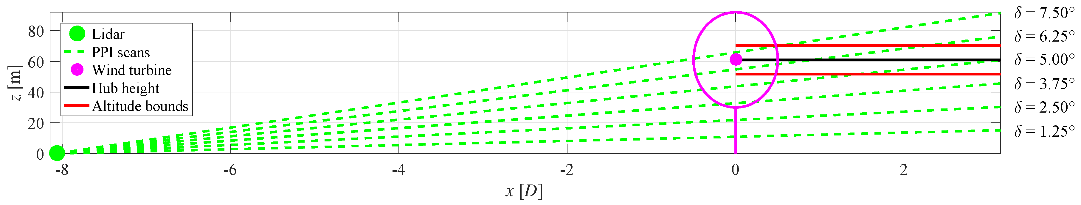
• A ‘volume scan’ based on six 30° azimuth sector PPI scans from each of the two lidars with elevations δ ranging from 1.25° to 7.5°. Note that this is not an actual volume that is spatially equally well covered in all directions, but a compromised way to gain volumetric information with a set of inclined PPI scans. Therefore, we refer to it as the ‘volume scan’ in the following.
• A single elevation, 30° azimuth sector PPI scan from each of the two lidars with $\delta =5°$. This scenario will be referred to as the ‘single elevation scan’ in the following.

Each of the lidars measures 46 range gates spread equidistantly over distances between 400–850 m. The azimuth angle resolution is 0.5° and the scanning speed is 1.25°·s${}^{-1}$. Both scenarios aim at measuring a horizontal wind field at hub height between 1D upstream and 3D downstream of the turbine rotor with ground-based lidars. The positions of the lidars should be chosen in order to have an appropriate relative azimuth angle $\Delta \chi$, i.e., the angle between the line-of-sight direction of the scanner of the different lidars, as to reduce the numerical uncertainty of the estimated wind vector. Stawiarski et al. [32] provide a thorough analysis on the effect of $\Delta \chi$ on the dual-Doppler lidar error. 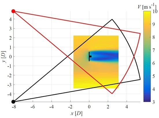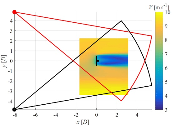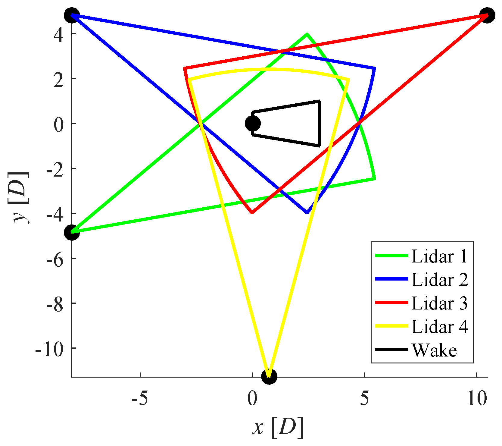Based on that work, a general recommendation is to avoid having two lidars pointing in the same ($\Delta \chi \approx 0°$) or opposite direction ($\Delta \chi \approx 180°$), since linearly dependent measurements are performed that way. The inclusion of the continuity equation in MuLiWEA is intended to mitigate this issue. Four different lidar placements are considered in the simulations, which could be combined to form both favourable and unfavourable measurement setups. A top view sketch of these lidar positions together with their corresponding simulated PPI scan sectors can be seen in Figure 3. The wind turbine is located at (0, 0), and its wake is roughly indicated with a black trapezoid. The volume scan is illustrated by the side view in Figure 4. Specific altitude bounds have to be selected to determine which measurements are taken into account to give an estimate of the wind speed at hub height. Therefore, a dimensionless parameter $C_h$ is defined, such that the altitude range is calculated by $h_h\pm C_h\frac{D}{2}$. The volume scan and the single elevation scan have $C_h$ values of 0.3 and 0.5, respectively. For both measurement scenarios, a radius of influence R of 6 m is used. These two parameters have been carefully defined through an error optimisation [33], the demonstration of which lies beyond the scope of this paper. Since the R value equals 1.5 times the grid resolution, the circles with radius of influence (see Figure 2) around different grid points overlap.

3.2. Real Dual-Doppler Lidar Wake Measurements

A case study on a measurement scenario executed in the German offshore wind farm “alpha ventus” is provided. Two Leosphere Windcube WLS200S long-range pulsed lidars (Orsay, France) were used to measure the wake of the AV10 (alpha ventus, number ten) Adwen AD 5-116 wind turbine (Adwen GmbH, Bremerhaven, Germany) by means of single elevation PPI scans. The lidars were installed on offshore platforms, resting on their four adjustable legs and mounted with additional tensioning belts. The turbine has a rated power $P_r$ of 5 MW, rotor diameter D of 116 m and hub height $h_h$ of 90 m. The same two lidars were previously used in a dual-Doppler configuration during an onshore measurement campaign. During that experiment, Schneemann et al. [34] compared the wind vector evaluated from a cup anemometer and a wind vane installed on a meteorological tower close to the lidar measurements with the horizontal wind vector computed from the radial speed measured by two lidars. This validation yielding goodness of fit values $R^2$ of 0.986 and 0.998 for the wind speed and wind direction in a free inflow sector, respectively.

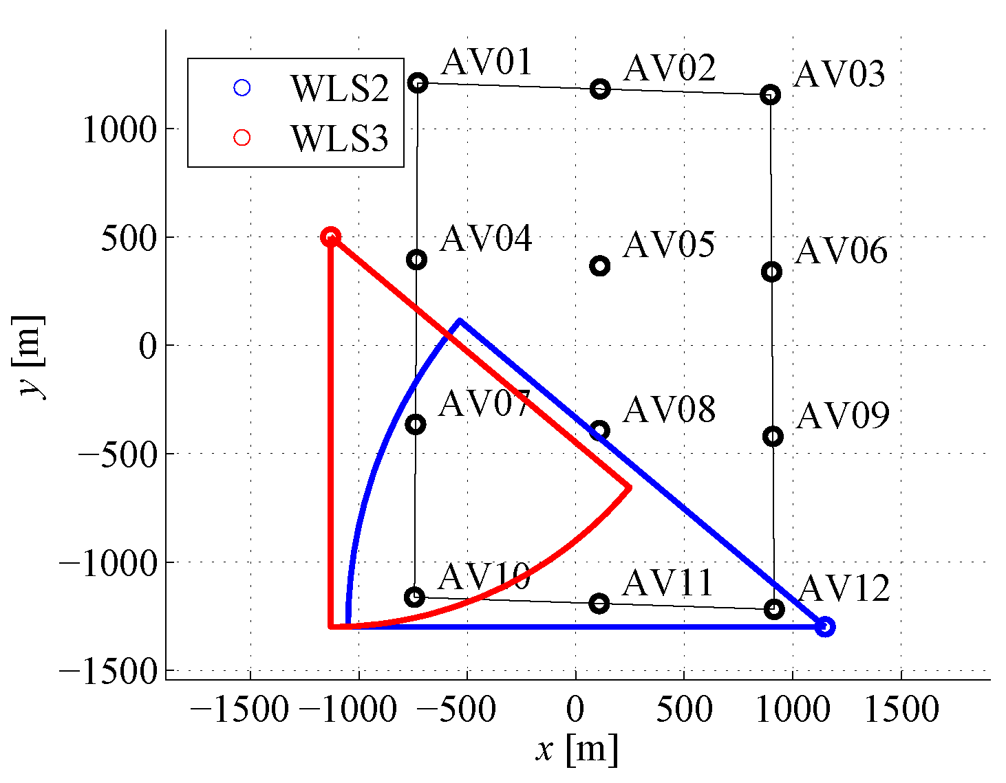
In Figure 5, a sketch of the measurement setup of the dual-Doppler lidar PPI scan scenario is depicted. These single PPI scans have elevation angles of 2.0° (WLS2) and 2.8° (WLS3), respectively. They cover an azimuth sector of approximately 30° with a resolution of 0.3°. For the application of MuLiWEA, measurements were selected with a $C_h$ value of 0.3, corresponding to an altitude range of (72.6, 107.4) m around the wind turbine hub height. The wind field resolution is 20 m, and the radius of influence is chosen to be 30 m. The measurements were filtered by their CNR values, by selecting measurements within a (−22, −8) dB range. This omitted both measurements with a high uncertainty because of a minor backscatter energy in the spectrum, thus a low CNR value, as well as measurements compromised by hard targets such as wind turbines, which can be distinguished by high CNR values.

4. Results

4.1. Simulated Dual-Doppler Lidar Measurement Scenarios

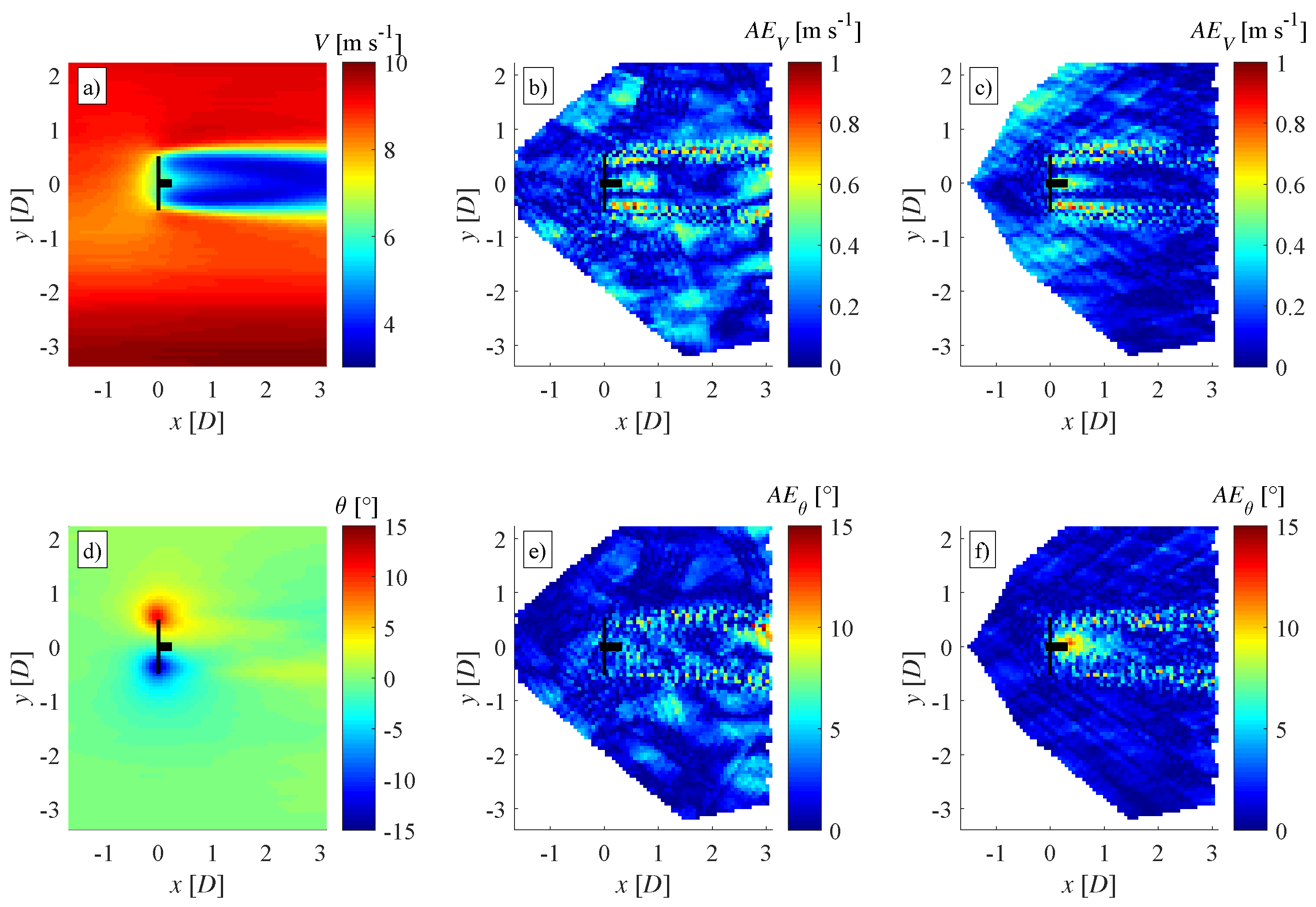
In Figure 6a, the absolute value of the 10 min horizontal wind speed at hub height over the LES-simulated wind field is shown. Absolute error plots of this wind speed are depicted in Figure 6b,c for the volume scan scenario and the single elevation scan scenario, corresponding to case 1 and 3 in

Table 1. Mean average error of the reconstructed wind field for different scenarios. Lidar selection refers to Figure 3 and the two highest and lowest values are marked red and green, respectively.

Case	Lidar Selection	Scanning Scenario	Continuity Correction	$\mathit{MAE}$ (m·s${}^{-1}$)
1	1 + 2	volume	on	0.171
2	$\Delta \chi \approx 60°$	volume	off	0.175
3		single elevation	on	0.156
4		single elevation	off	0.158
5	1 + 3	volume	on	0.379
6	$\Delta \chi \approx 180°$	volume	off	1.793
7		single elevation	on	0.443
8		single elevation	off	1.688
9	2 + 3	volume	on	0.157
10	$\Delta \chi \approx 120°$	volume	off	0.163
11		single elevation	on	0.124
12		single elevation	off	0.124
13	2 + 4	volume	on	0.216
14	$\Delta \chi \approx 120°$	volume	off	0.254
15		single elevation	on	0.160
16		single elevation	off	0.171

, respectively. Grid points are only included when there was at least one measurement from each of the lidars available locally. The absolute error patterns of the two different scenarios both show similar significant errors of up to 1 m·s${}^{-1}$ on the boundaries of the wake. These are characterised by large velocity gradients, which are smoothed by the averaging of the single lidar line-of-sight measurements over their probe volumes, the weighted averaging of the measurements over the circular area with radius of influence, taking into account measurements from different heights and the temporal averaging.

For each of the considered cases listed in Table 1, the mean average error on the absolute wind speed ($MAE$) is calculated from the corresponding absolute error plots (see Figure 6b,c). This enables the assessment of different combinations of lidar placement, different PPI scan scenarios and the effect of the continuity correction. Based on the $MAE$, the most favourable scanning scenario is the single elevation scan. The best lidar configuration in this case is using lidar 2 and 3 (see Figure 3). The continuity equation always has a positive influence, but the improvement is largest for the least favourable combination of lidar locations. Namely, in the case of combining lidars 1 and 3, a part of the measurements from both lidars lie on the same line-of-sight ($\Delta \chi \approx 180°$) and are therefore linearly dependent.

The 2D wind field description is completed by the wind direction, which is represented by Figure 6d for the LES. Again, the absolute error on the wind direction can be seen in Figure 6e,f for the two aforementioned scenarios. Note that westerly wind is described as a relative angle $\theta =0°$ here. It can be observed that the flow is locally deflected with up to $\pm 15°$ as it passes the wind turbine rotor and then gradually aligns with the initial wind direction further downstream. For both measurement scenarios, the deflection around the wind turbine is captured well.

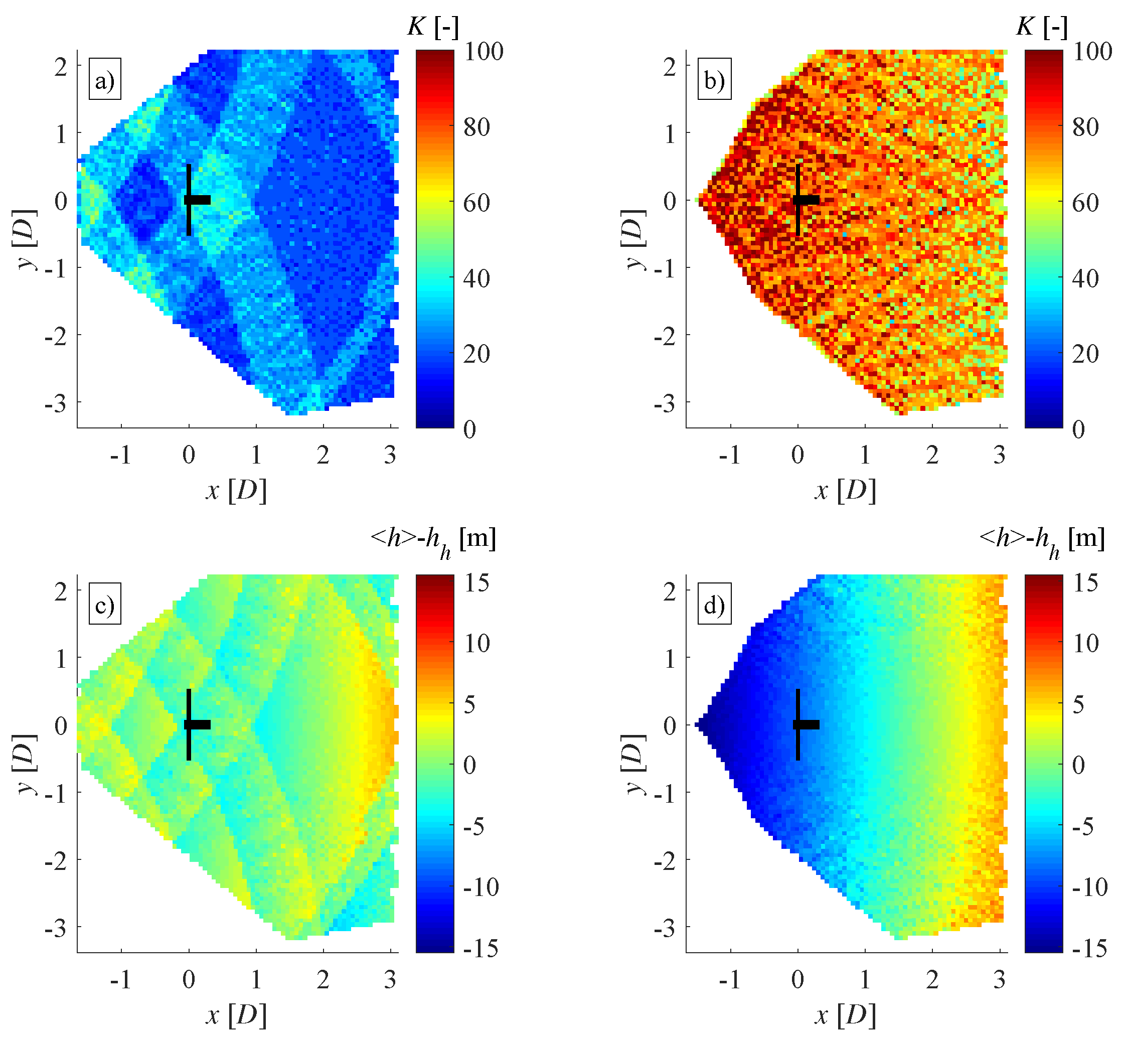
However, local errors can be noticed on the absolute error plots in Figure 6e,f, caused mainly by two reasons: the first issue is the intrinsically heterogeneous measurement distribution of the radial scan pattern of the lidars. Second, the average height at which measurements were taken causes a problem. Especially for the volume scan scenario, these two effects are entangled. Figure 7a,b show the measurement distribution, i.e., the number of measurements K taken into account per grid point, for the two respective scenarios. Figure 7c,d illustrate the average offset from hub height of the measurement set for each grid point.

The measurement distribution of the single elevation scan corresponds to the radial scanning pattern. Since the lidars are both located to the west, the distribution becomes less dense when progressing radially outward, i.e., from west to east. The measurement distribution of the volume scan is relatively heterogeneous due to the combination of multiple, partly overlapping PPI scans. However, it shows smaller absolute quantities than the single elevation scan and also has a larger spread in the count of measurements over the grid. For the single elevation scan, the average height offset from hub height is linearly increasing from west to radially outward. The volume scan approaches the hub height more convincingly, i.e., the average absolute offset of the measurements is much lower, namely 1.6 m instead of 6.8 m. However, due to the heterogeneous pattern, some local peaks and sharp discontinuities are present.

The large absolute errors on both the absolute velocity and the wind direction estimated by the volume scan to the far east of the measurement domain (see Figure 6b,e) are possibly caused by an average height difference of 8 m locally (see Figure 7c). The error in the wind direction directly east of the wind turbine in case of the single elevation scan (see Figure 6f) is most probably caused by the average height difference of 10 m locally (see Figure 7d). Alternatively, wake-induced v-components combined with the spatial averaging applied in the algorithm could also be the reason of the observed absolute errors in the wind direction.

4.2. Real Dual-Doppler Lidar Wake Measurements

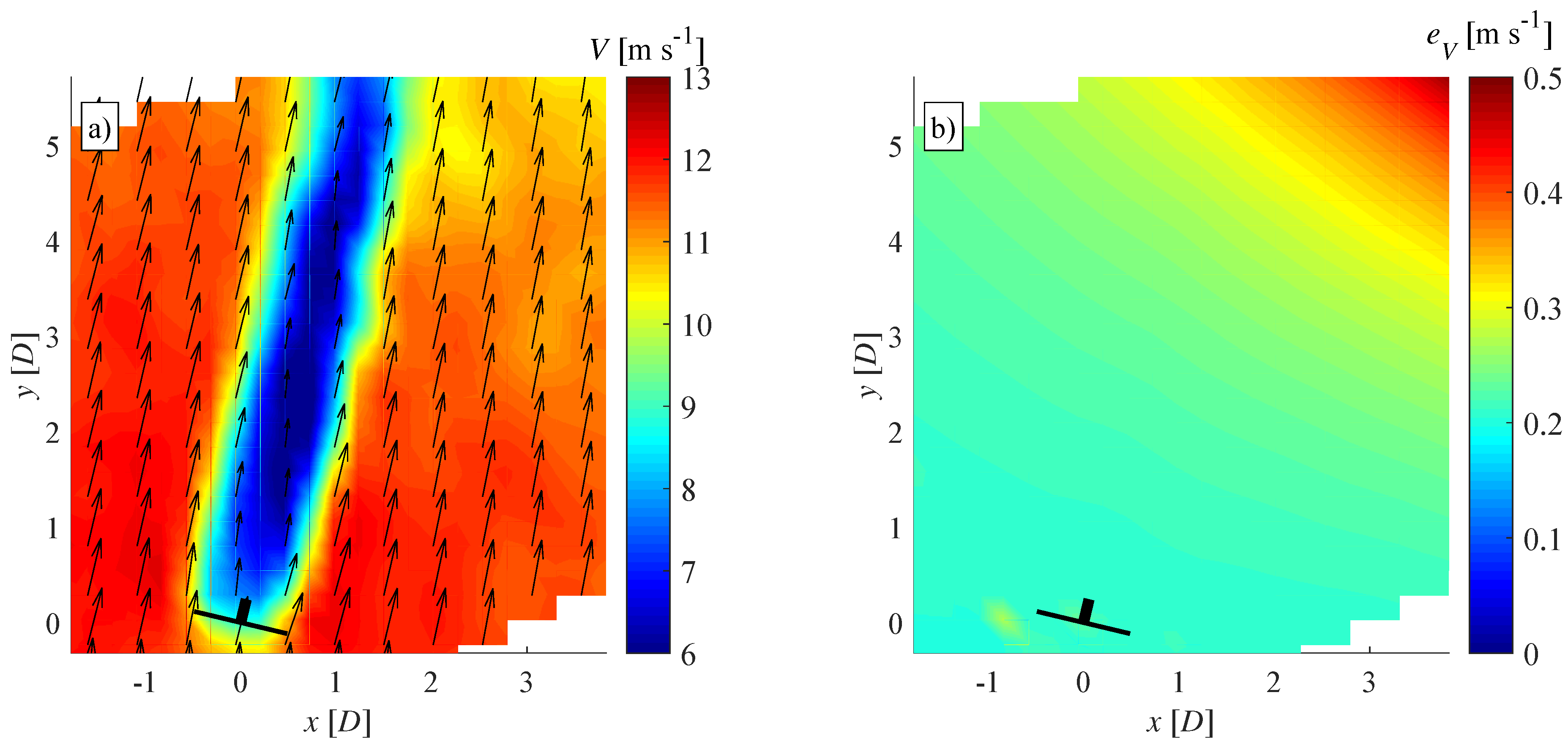
Figure 8a shows a 10 min wind field reconstructed by MuLiWEA, from data collected on 20 February 2014 at “alpha ventus”. Within this time interval, the lidars cover the PPI sectors indicated in Figure 5 seven (WLS2) and five (WLS3) times, respectively. According to data from the FINO1 measurement mast (Forschungsplattformen in Nord- und Ostsee Nr. 1), a southerly wind (181.7°) with an undisturbed speed of 11.16 m·s${}^{-1}$ and a turbulence intensity of 5.88% at hub height were prevailing at the time. The wind turbine was operating under its rated conditions. In Figure 8b, the absolute error on the wind field can be seen. The basic error on the line-of-sight velocity is built up by the lidar measurement error and the numerical uncertainty of MuLiWEA. The lidar $v_{LOS}$ uncertainty and pointing error are 0.2 m·s${}^{-1}$ and 0.11°, respectively, according to the manual from Leosphere. The numerical uncertainty is estimated through analysis of the residuals of the linear system in Equation (7). Uncertainty propagation is used to combine all mentioned error sources to provide an estimate of the absolute error on the reconstructed wind vector value V. This approach is explained in detail in Appendix A. Note that the wind field estimation within ±1D longitudinal distance of the wind turbine has a relatively high uncertainty due to laser signal reflection from the wind turbine. In the averaged wind field, no significant fluctuations in wind direction can be distinguished further downstream of 1D. However, the error shows an increasing trend towards the northeast, which is directly related to the relative azimuth angle $\Delta \chi$ of the lidars. In the wake of the wind turbine, slight negative direction deviations were noticed, most probably caused by the wake rotation that is impacting the horizontal wind speed at measurement heights above the hub height. More results from this measurement campaign were compared with LES by Vollmer et al. [35], which confirms the usefulness of the algorithm in combination with the measurement campaign for steady wake model validation on a 10 min basis.

5. Discussion

A problem with applying lidar to small scale meteorological phenomena is the spatial probe length averaging effect. In addition, the MuLiWEA performs spatial and temporal averaging of the measurements. These effects combined hinder capturing large velocity gradients that commonly occur on the boundaries of wakes. However, the algorithm resolves the wake with sufficient accuracy to determine e.g., its deficit and width. Because of the limitation on time resolution, it is not possible to investigate wake or boundary layer dynamics with the scanning speed of the currently available lidars using asynchronous PPI scans. This limitation could be overcome by synchronising the lidars or improving their temporal resolution. In the current situation, the target application of the algorithm is steady wake model validation on a 10 min time scale.

The rotation of the near wake induces unsteady lateral and vertical wind speed components. This increases the uncertainty of a reconstructed wind field in case PPI scans are not executed horizontally at hub height but with varying altitude offsets. In particular, a significant deviation was observed in the wind direction for measurements taken at a distance from hub height. However, the effect on the absolute horizontal wind speed is negligible. Because the rotation of the wake is a deterministic phenomenon, it could be accounted for by the algorithm, in a similar way as the continuity adjustment was implemented.

Because the simulated lidar measurements were modeled to a perfect accuracy, most of the errors in the investigated dual-Doppler lidar scenarios are indirectly a result of the irregular sample distribution over the height, which does not perfectly resemble the hub height at all locations on the horizontal plane.

Although it was argued and proven by the error analysis that neglecting the vertical velocity component does not significantly increase the uncertainty of the reconstructed wind components, a valuable extension to MuLiWEA could be the inclusion of the vertical component. For this purpose, additional lidars are needed that measure with relatively high elevation angles.

Only a single 10 min reconstructed wind field was provided in the real measurement application section. This was mainly meant to illustrate the difference with respect to a simulated case and serve as an example. Further analysis of actual measurements, preferably with reference anemometry, could assist with evaluating the algorithm properly.

6. Conclusions

MuLiWEA was developed to increase the potential of reliable lidar measurements of wind turbine wakes and is suitable to reconstruct two-dimensional wind fields based on measurements from multiple-lidar PPI scanning scenarios. Different ground-based dual-Doppler lidar PPI scenarios were simulated and applied on a LES wind field with a wind turbine wake. An evaluation on the mean averaged error of the absolute horizontal wind speed for the different simulated cases showed that the single elevation scan always provides more accurate results. This type of scan, which intersects the hub height at a given location, will provide measurement height offsets at other positions, but the distribution of the measurement points will be relatively homogeneous. Executing multiple PPI scans with varying elevation angles offers the possibility to decrease the altitude range and therefore the reconstructed wind field is more representative of the one at hub height. The downsides are that the measurements are spread more heterogeneously over the grid, and that full coverage of the area takes longer than with a single elevation scan, yielding less measurement points within fixed time frames. Especially in a highly turbulent wake this can induce errors.

From the error analysis on the simulated dual-Doppler lidar scenarios, it was proven that, if PPI scans with low elevation angles are used, the vertical wind speed component has a negligible effect on the absolute error of the reconstructed wind field.

The inclusion of the continuity equation in the MuLiWEA generally improves the accuracy of the reconstructed wind field. Especially in case the measurements from the two lidars are linearly aligned, the mean absolute error is decreased significantly.

A dual-Doppler lidar measurement scenario in “alpha ventus” was considered to test a first real application of MuLiWEA. Unfortunately, there is no suitable reference to validate the reconstructed wind field, and some small angular sectors are blocked by the towers of the wind turbines. These measurements were filtered out and cause local data scarcity, increasing the uncertainty. Despite of these challenges, the application of MuLiWEA to dual-Doppler lidar PPI measurements of wind turbine wakes was successful and further development is promising.