Article

Creating Multi-Temporal Composites of Airborne Imaging Spectroscopy Data in Support of Digital Soil Mapping

Remote Sensing Laboratories (RSL), University of Zürich, Winterthurerstrasse 190, Zürich 8057, Switzerland
*
Author to whom correspondence should be addressed.
Remote Sens. 2016, 8(11), 906; https://doi.org/10.3390/rs8110906
Submission received: 19 July 2016 / Revised: 5 October 2016 / Accepted: 27 October 2016 / Published: 2 November 2016
(This article belongs to the Special Issue Remote Sensing Applied to Soils: From Ground to Space)

Abstract

:
An increasing demand for full spatio-temporal coverage of soil information drives the growing use of soil spectroscopy. Soil spectroscopy application performed under laboratory conditions or in-field studies in semi-arid areas have shown promising results. However, when acquiring data in temperate zones, limitations by vegetation-free coverage, variation in soil moisture and management are driving coherent spatio-temporal data collection. This study explores the use of multi-temporal imaging spectroscopy data to increase the total mapping area of bare soils in a heterogeneous agricultural landscape. Spectrally and spatially high-resolution data from the Airborne Prism Experiment (APEX) were collected in September 2013, April 2014 and April 2015. Bare soils in all acquisitions were identified. To eliminate short-term differences in soil moisture and soil surface roughness, the empirical line method was used to calibrate the reflectance values of the singular images (2013 and 2015) towards the singular image with most bare soil pixels (2014). Difference indicators show that the calibration was successful (decrease in root mean square difference and angle difference, increase in R2 and gain and offset close to one and zero). Finally, the multi-temporal composite image contained more than double the amount of bare soil pixels as compared to a singular acquisition. Summary statistics show that reflectance values of the multi-temporal composite approximate the single image data of 2014 (mean and standard deviation of 2014: 24.2 ± 8.9 vs. 24.0 ± 9.5 for the multi-temporal composite of 2013, 2014 and 2015). This indicates that global differences in soil moisture and land management have been corrected for. As a result, an improved spatial representation of soil parameters can be retrieved from the composite data. Spatial distribution of the correction factors and analysis of the spatial variability of all images, however, indicate that non-linear, short-term differences like variation in soil moisture and land management largely influence the result of the multi-temporal composite. Quantification and attribution of those factors will be required in the future to allow correcting for them.

Graphical Abstract

1. Introduction

“Soil is a complex material that is extremely variable in its physical and chemical composition” [1]. Large variability of soils is caused by interactions of: (I) environmental factors [2], which influence inherent soil properties (i.e., texture) and thus control soil formation; and (II) human influence [3], which controls dynamic soil properties (i.e., structure, organic matter) over the course of years in response to land use and land management. Understanding the soil as a complete system, including its mechanisms and processes is difficult. However, this is important for policy-making, land resource management and monitoring the environmental impact of development. Spatially distributed soil information has become more important with the use of global and regional models, which often require full coverage soil information [4]. Conventional soil sampling and laboratory analysis, however, are time consuming, costly, and because of different standards, often inconsistent [4,5]. Therefore, these methods cannot efficiently provide this information [6,7].
The growing need for low-cost, standardized and large-scale spatial soil data results in the requirement for alternative methods. The use of remote sensing can offer spatial and temporal, quantitative soil information of extended areas [8], which can be acquired with limited fieldwork. Therefore, remote sensing has the potential to: (I) support the design of sampling schemes; (II) physically and empirically derive soil properties; (III) provide support for digital soil mapping; and (IV) facilitate large-scale spatial information even in inaccessible areas [4,5,6,7]. However, the knowledge of how to apply remote sensing in soil mapping is still incomplete and several disadvantages are known. Single or even multi-band remote sensing is limited when striving for quantitatively accurate information, because the spectral features of soils are largely weak, narrow and mixed. High spectral resolution data are required to give qualitative and quantitative information on soils. Furthermore, remote sensing cannot detect the entire soil horizon, but is limited to the thin upper layer of the soil (topsoil). However, the upper soil horizon contains valuable information about the soil, which can be utilized by farmers and decision makers [8].
Compared to traditional methods of soil mapping, soil spectroscopy gives information that is especially interesting at small scales. The detailed information that can be provided by soil spectroscopy is information that is not easily gained with other (traditional and modern) methods [8,9]. There are many examples that show the successful use of soil spectroscopy (e.g., [10,11,12,13,14], for a comprehensive list we refer to [4]). However, soil spectroscopy research still has a strong focus on laboratory conditions [15]. Fewer studies apply in-field soil spectroscopy (e.g., [6,16,17,18], only about 10% [15]) and these studies are mainly located in (semi-) arid areas or applied to single fields. In this way, they avoid the challenges in-field soil spectroscopy is facing when applied outside of these areas [19]. Soils in-situ are varying [20] as a consequence of changing meteorological conditions and land management practices. This results in variations in: (I) soil surface coverage, both vegetation and residual cover; (II) soil moisture; and (III) soil surface roughness. These short-term variations in soil surface conditions are mentioned as the main challenges for in-field application of soil spectroscopy [19,21].
Partial or complete coverage of the topsoil by vegetation disturbs the signal of bare soils drastically. Therefore, using direct sensing conditions [8] i.e., excluding all covered parts—offers the best predicting solution [4]. However, these bare soil areas in a temperate climate are sparse. Nevertheless, Lagacherie et al. [9] conclude that there is a need to increase the amount of bare soil area, before dealing with permanently vegetated areas. Crop rotation in agricultural areas can offer an opportunity to increase the area of bare soils under direct sensing conditions, which was already suggested by Gerighausen et al. [22].
In central European agricultural areas, most soils are bare in early spring, just before or after sowing of summer crops; and in late summer, just after harvesting and just before or after sowing of winter crops [22]. Multi-temporal spectroscopy data from early spring and/or late summer can therefore offer a possibility to increase the area of bare soils. Unfortunately, sowing and harvesting occurs within a period of several weeks up to some months because of meteorological conditions and the farmer’s decision. Furthermore, not only sowing and harvesting is dependent on meteorological conditions, also the collection of airborne spectroscopy data is weather dependent. Therefore, it is only possible to select periods with a high probability of a large amount of bare soils and try to collect data in these periods. Upcoming multispectral and imaging spectroscopy satellite missions will provide freely available imaging spectroscopy data with a short return period and will likely solve this problem (e.g., European Sentinel 2B (2017) [23], German EnMAP (2018) [24], Italian PRISMA (2018) [25], Japanese HISUI (2018) [26], Italian-Israeli SHALOM (2021) [27], and American HyspIRI (2022) [28]). This makes the use of multi-temporal spectroscopy data even more interesting.
In contrast to Gerighausen et al. [22], who created a mosaic of multi-annual soil property estimations, we propose to create a multi-temporal composite of the spectroscopy data to increase the total area of bare soils. Since inherent soil properties (e.g., texture) mainly change on the long-term [2] and more dynamic properties (e.g., structure or organic matter) over the course of years, we approximate that the soil properties of interest remain static within a time frame of several years. Differences between the reflectance data of the same bare soil pixel in multiple years are mainly caused by processes varying on short time scales, including weather conditions influencing soil moisture and land management practices and precipitation events influencing soil surface roughness. Therefore, combining multi-temporal spectral data comes with the challenge of correcting for spectral variation caused by these processes.
It is known that spatial variation in soil surface conditions decrease the accuracy when deriving soil properties from spectroscopy data [29]. Much research has been done on quantifying and removing these effects from the soil spectra [1,19,20,29,30,31,32,33,34,35,36,37,38,39,40]. However, most research is focused on the effect on specific soil properties (e.g., [34,36]); focus only on specific spectroscopy techniques (e.g., [35]); or are laboratory based (e.g., [33]). Surely, these studies have resulted in valuable information on the effect of soil moisture and soil surface roughness on spectroscopy data. For soil moisture it is known that the reflectance decreases with higher soil moisture, the water absorption features at around 1400 and 1900 nm are more affected than the rest of the spectra [20,36,37,40]. For soil surface roughness it is known that for increasing roughness, the reflectance is generally lower, due to self-shadows [19,32,33]. Eliminating these short-term processes of meteorology and land management is necessary in order to use a multi-temporal composite for deriving soil properties.
The aim of this study is to create a multi-temporal composite of spectroscopy data in order to improve the application of soil spectroscopy in a heterogeneous, temperate environment. For this we focus on how to deal with short-term processes of meteorology and land management resulting in differences in soil moisture and soil surface roughness. Within the next chapters we show: (I) how the multi-temporal composite was created based on the empirical line method; (II) the analysis of the spectral quality of the calibration and of the multi-temporal composite compared to the single acquisitions; and (III) the potential of this methodology for digital soil mapping based on a case study in which we compare the predictions of sand percentages for the single acquisitions and the multi-temporal composites.

2. Study Area and Soil Types
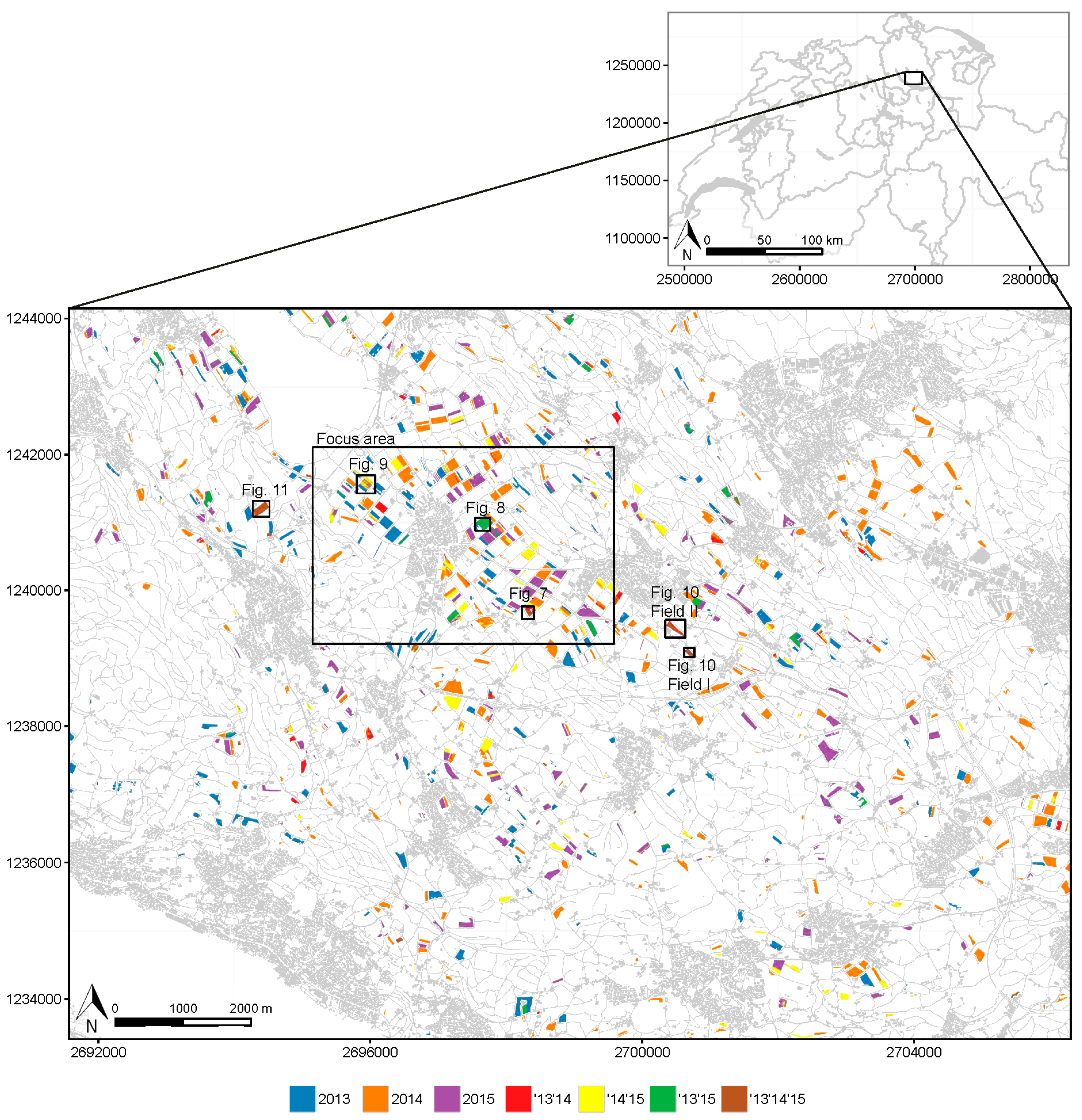
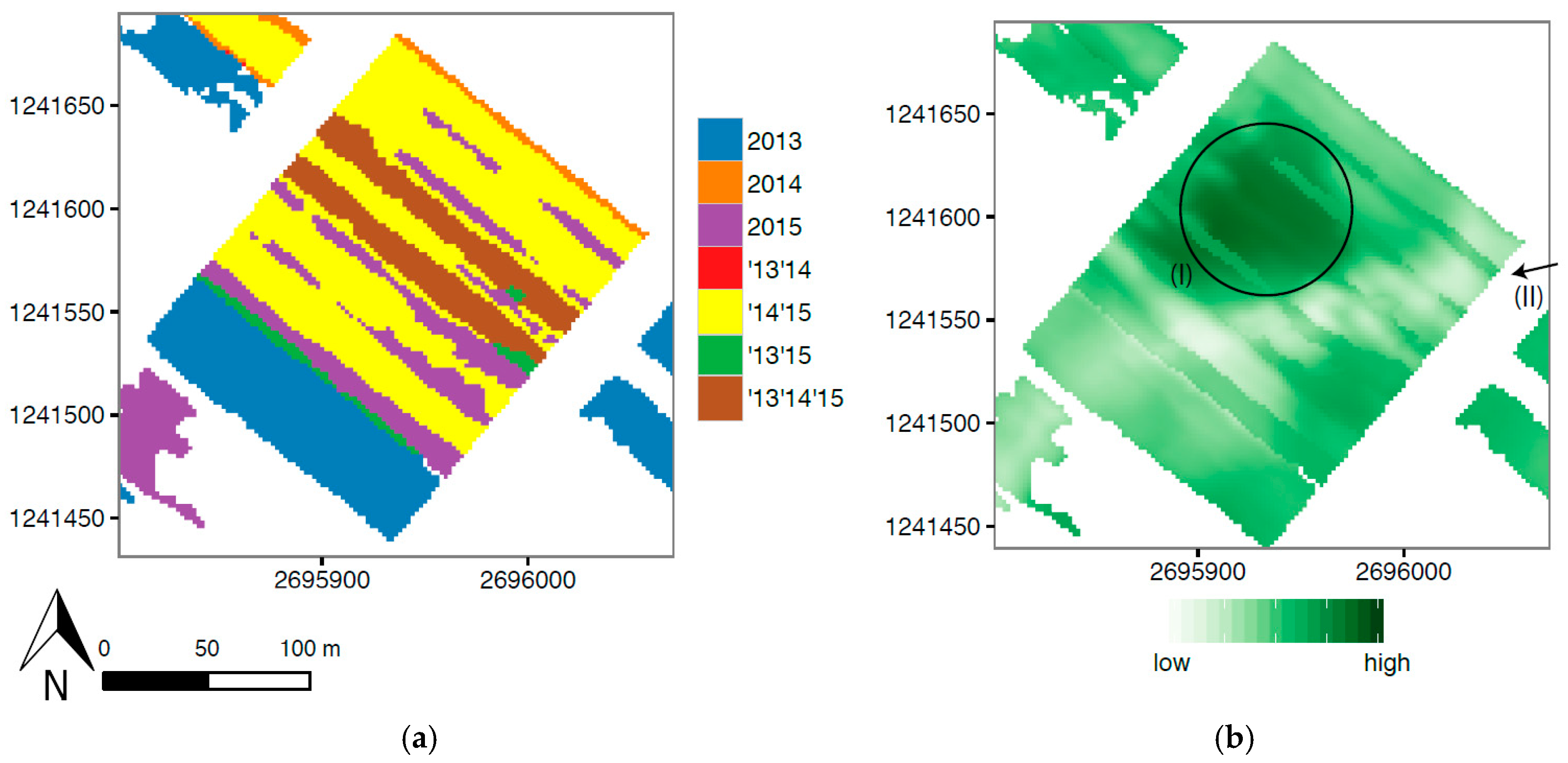
The study area (Figure 1) is located in the Canton of Zurich (Switzerland), southeast of lake Greifensee. This area was repeatedly covered by oceans (Jurassic times), resulting in layers of marlstone, limestone, and sandstone. During the Alpine orogeny this site was part of a foreland basin (Molasse basin), where sediments (sandstone, siltstone, marlstone, limestone and conglomerates) from the developing mountain chain were collected. During the Quaternary, the ice ages formed the landscape in the Swiss highlands. Glaciers repeatedly covered the Swiss plain and created a landscape with typical glacier landforms, like moraines, drumlins, and lakes [41].
The available soil map [42] and literature [43,44,45] show that the soils underlying the area reflect the geologic history. Soils are classified as clay loam or loam and contain a lot of silt (sand, silt, clay, respectively around 30%, 40%, 30%). Soils contain high amounts of organic matter (on average around 10% in the upper 10 cm) as a result of former impermeable peat soils (now drained); and some of the soils contain lime. In the lower areas, soils can be found that, without drainage, would be saturated with groundwater and pendular water. Redox processes result in gleyic color patterns Gleyic Cambisols (Braunerde-Gley), Gleysols (Buntgley and Fahlgley), and Histosols or Histic Cambisols (Halbmoor). Because of the influence of the glaciers, which resulted in dense, impermeable layers, many Planosols (Braunerde-Pseudogley and Pseudogley) can be found in the area as well. Other areas are dominated by mineral Cambisols ((Kalk-Braunerde), which are characterized by a clear soil formation (A, B and C horizon). Furthermore, there are few Regosols in the area, these shallow and poorly developed soils are mainly found on rock outcrops [43,44,45].
The area contains a valley with a small glacial lake (Greifensee) and two ridges in the northeast and southwest, both are northwest to southeast oriented. The elevation of the area ranges from ca. 405 m in the valley to ca. 845 m on the ridge in the southwest and to 930 m on the ridge in the northeast [46]. The lower areas are dominated by cropland and (temporary) grasslands. As a result of direct payments, crop rotation is promoted to cover bare soils in winter to protect against soil erosion. Consequently, the croplands are dominated by winter cereals and rapeseed; furthermore, maize and some summer cereals and vegetables can be found. Table 1 shows the sowing and harvesting periods for the most dominant crops in the study area. The hilly areas in the northeast, southwest and towards the southeast are less suitable for agricultural purposes because of their hilly character and are mainly covered with (permanent) grasslands or (mixed) forest.
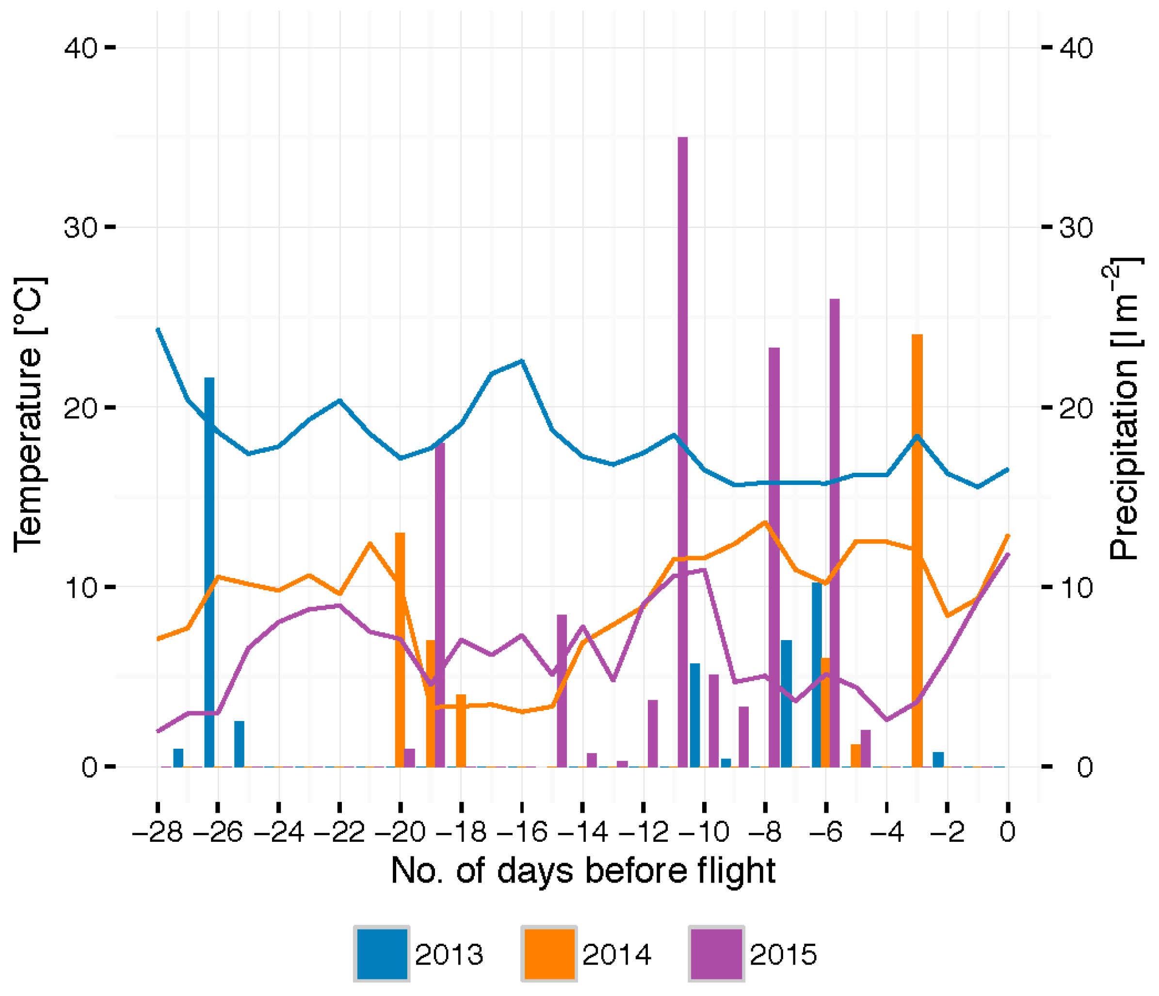
The climate can be classified as a warm temperate humid climate (warmest month lower than 22 °C average, minimum of four months above 10 °C on average). Summers can be hot, with temperatures reaching 30 °C. The area around Zürich receives around 1000 mm of annual precipitation on average. Precipitation is evenly distributed over the entire year, peaking in June and August. Winters are cold, but snow is only occasionally falling in the area, which instead experiences fog during this period.

3. Materials and Methods

3.1. Preprocessing of Imaging Spectroscopy Data

The Airborne Prism Experiment (APEX) is an airborne imaging spectrometer developed by a Swiss–Belgian consortium on behalf of ESA [48]. The instrument is a dispersive pushbroom imager with a 28° field of view. The instrument is composed of two spectral channels, of which each has a given number of spectral bands. The channels cover the spectral range from 372–2540 nm with 1000 across track pixels. Depending on the flight altitude, the ground pixel size ranges from 1.5–2.5 m. The unbinned configuration offers 312 spectral bands in the visible and near-infrared (VNIR) and 199 bands in the short-wave infrared (SWIR) region of the electromagnetic spectrum [49,50].
According to the seed and harvest periods shown in Table 1 the best period to collect bare soil spectral data is in early spring for summer crops (e.g., maize) and late summer/early autumn for winter crops. Since, spectroscopy data can only be collected under clear meteorological conditions the flight windows were set for both early April and September. Finally, APEX data were acquired on 3 September 2013, 11 April 2014 and 10 April 2015 (for brevity, we refer to these images as ’13, ’14 and ’15 respectively when used in difference images or in multi-temporal composites). All data have been atmospherically corrected and orthorectified [51], resulting in a surface reflectance (level 2) data cube of 284 bands ranging from 400–2400 nm, and a spatial resolution of 2 × 2 m2. Subsequently, the following spectral bands were removed because of (I) interpolated bands: 691.0–735.9 nm; 752.9–770.8 nm; 794.9–838.0 nm; 900.4–992.1 nm; 1072.4–1166.5 nm; 1283.0–1495.7 nm; 1738.7–2028.7 nm; and (II) low signal to noise (SNR) bands: below 450 nm and above 2200 nm. This means that, e.g., clay cannot be determined by typical absorption features at 2200 nm, however there is no scientific purpose to apply noisy data to such an analysis.

3.2. Selecting Bare Soil Area

Spectral indices were used to mask green vegetation (normalized difference vegetation index (NDVI) [52,53]), water (normalized difference red blue index (NDRBI) [54,55]), and residual vegetation (normalized cellulose absorption index (nCAI) [56]). Based on these indices a soil dominant mask was created with help from the software HYSOMA [57], the default settings and thresholds were used. Separation between built-up area and the bare soils was performed using auxiliary data. For this, we used the agricultural field block map [58], which was updated based on available built-up footprints [59] and road information [46] by swisstopo. For further analysis, the overlapping bare soil pixels between the images of 2013, 2014 and 2015 were selected.

3.3. Multi-Temporal Calibration

In order to correct for the differences between the reflectance values of the same pixel in multiple years, caused by short-term processes, we have used the empirical line method [60]. The empirical line method is a methodology traditionally used for atmospheric correction of remotely sensed data from at-sensor radiance to at-surface reflectance, assuming that within the image one or more targets are present covering a wide range of reflectance values. At-surface reflectance measurements were taken and compared to the at-sensor radiances for each wavelength. This resulted in a calibration equation that predicts at-surface reflectance from at-sensor radiance [61]. The actual calibration was done by multiplying the at-sensor radiance by the gain factor and adding the corresponding offset [62]. The use of more targets resulted in a more accurately determined linear relationship between at-sensor radiance and at-surface reflectance, and therefore more accurate estimation of the gain and offset used for calibration [61]. We consider the overlapping bare soil pixels as indifferent targets within these three years and use them as input for the calibration model. Consequently, the overlapping bare soil pixels were used to calculate a linear regression that was used to create a calibration model. A separate calibration model was created for each wavelength. As a reference year we used 2014, which was the scene with the largest bare soil area. The calibration curve was calculated according to Equation (1).
R r e f , i = α i + β i · R c a l , i
where R is the reflectance (%) for the reference year ref and the calibration year cal, α is the offset and β is the gain of the linear correlation, i is the considered wavelength. The offset and gain values from this linear correlation are used to correct the reflectance values (Rcor) of the calibration year:
R c o r , i = α i + β i · R c a l , i
In order to calculate robust calibration models, we removed outliers for each calibration model based on Cook’s distance (see Section 4.2). Cook’s distance [63] is an estimation of the influence of a data point on the least squares regression. It therefore not only considers the data points with large residuals (outliers), but also data points with a high leverage. These points are known to have a large influence on the outcome and the accuracy of the regression model (R2, RMSE, gain and offset values, etc.). Cook’s distance (Di) is based on the relation between the studentized residuals (ei) and the measure of leverage (hi) of a data point, which results in Equation (2).
D i = e i 2 p · M S E [ h i ( 1 h i ) ]
where MSE is the mean squared error of the calibration model and p the number of independent variables (in our case only one). Outliers were removed based on the rule-of-thumb [64] of:
D i > 4 n

3.4. Analysis of the Multi-temporal Calibration

3.4.1. Difference Analysis

The overlapping pixels were used to analyze the differences between the bare soil spectra of the three years. Differences between the spectra were analyzed based on two indicators [65]: (I) the root mean square difference (D) between two spectra (Equation (5)); and (II) the difference angle (θ) between two spectra (Equation (6)), where θ normalizes for differences in offset.
D = 1 n 1 i = 1 n ( R x ( λ i ) R y ( λ i ) ) 2
θ = cos 1 ( i = 1 n R x ( λ i ) · R y ( λ i ) i = 1 n R x ( λ i ) 2 · i = 1 n R y ( λ i ) 2 )
where R is the reflectance value (%) at wavelength λi of the spectra of year x and year y, and n is the number of spectral intervals. Price [65] calculates Equation (6) with integrals instead of summations. We approximate integration using summation, which is a valid approach when using rectangular response functions. The imaging spectroscopy data are processed in such a way that it supports to use summation as an approximation for integration.
Besides this, we considered the linear correlation (Equation (7)) of the spectra between the years. In case of small differences between the reflectance (R) of overlapping bare soil pixels (j) in multiple years, correlation values are close to the one-to-one line with, trivially, an offset (α) of zero and a gain (β) of one.
R y , j = α j + β j · R x , j
for the year combinations ‘13’14 and ‘15’14, the first year is year y and the second year is year x. Based on these linear correlations also the coefficient of determination (R2) was calculated.
Summary statistics (mean and standard deviation), the difference indicators and the results of the linear regression between two years were calculated for the data without outliers (see Section 4.2.) and both before and after calibration. Since soil properties can be derived from specific parts of the spectrum—e.g., clay can be determined by its typical hydroxyl absorption feature at 2200 nm (e.g., [66,67]) and the visible part of the spectrum is closely related to the amount of organic matter in the topsoil (e.g., [68])—it is interesting to have a closer look at the effect of the calibration on specific parts of the spectra. Therefore, the summary statistics were not only calculated for the full spectra but also separately for the visible (VIS: 450–700 nm), the near-infrared (NIR: 700–1400 nm) and the short-wave infrared (SWIR: 1400–2200 nm) ranges of the spectra.

3.4.2. Spatial Analysis

In order to assess the differences between the original and the calibrated images spatially, we calculated the symmetric mean (absolute) percentage error (SM(A)PE) [69]:
M A P E = i = 1 n | R c o r , i R o r g , i | i = 1 n | R c o r , i + R o r g , i |
S M P E = i = 1 n R c o r , i R o r g , i i = 1 n R c o r , i + R o r g , i
where R is the reflectance (%) for the original (org) and the corrected (cor) value per band (i). We calculated this error both for the absolute differences (SMAPE) and the relative differences (SMPE), since it is interesting to see if the reflectance values were corrected positively (moving upwards) or negatively (moving downwards). The values are between 0 and 1 for the SMAPE, and between −1 and 1 for the SMPE, were 1 indicates 100% difference and 0 indicates no difference. Furthermore we calculated the SM(A)PE also for the VIS (450–700 nm), NIR (700–1400 nm) and SWIR (1400–2200 nm) ranges.

3.5. Multi-Temporal Compositing

The multi-temporal composite was then created, using a maximum bare soil pixel approach, by overlapping the corrected images. In case of soil pixels present in more than one year, the image with most bare soil pixels had higher priority. We then calculated the mean and standard deviation for the whole image for all individual images (2013, 2014, and 2015) and for all multi-temporal composites (‘13’14, ‘14’15, ‘13’15, and ‘13’14’15).

3.6. Analysis of the Multi-Temporal Composites

We transformed the data with a principal component analysis (PCA) [70,71] to analyze the spatial variability of the images of the different years. This means that a large set of correlated variables can be summarized with a smaller number of representative variables (principal components (PCs)) that together explain most of the variability in the original set [72]. This makes PCA especially useful when a large amount of correlated predictor variables (like imaging spectroscopy data) are present [73,74]. PCA was calculated using the R-package stats [75].
Based on the first PC of the PCA for each image, we calculated variograms [76], which indicate the correlation between distance and data values. The variance (γ(xi,yi)) was calculated based on Equation (9):
γ ( x i , y i ) = 1 2 n i = 1 n ( ( z ( x i ) z ( y i ) ) 2
where n is the number of pairs of sample points in the respective distance and angle class, z is the data value, and xi and yi are the spatial locations. The spatial dependency can be plotted as a variogram with γ(xi,yi) against yi − xi. Since we expect anisotropy, yi − xi is in this case not equal to h (a vector in distance and angular class yi − xi). The characteristics of the variogram are described as: (I) the sill, which is the variance at which there is no spatial dependence between the data (or random field); (II) the range, which is the distance at which there is no spatial dependence between the data; and (III) the nugget, which is the measurement error or micro-scale variation of the data (value of γ(xi,yi) at yi − xi = 0).
In order to explore the small-scale dependency we calculated, based on the first PC of the singular images (2013, 2014, and 2015), variograms for three agricultural fields that were present in all three years. Large-scale spatial dependency was explored by calculating variograms for the first PC of the singular images (2013, 2014, and 2015) and of the multi-temporal composites (‘13’14, ‘13’15, ‘14’15, and ‘13’14’15). Since it was computationally not possible to calculate the variograms based on all bare soil pixels present in the singular and multi-temporal images we calculated the variograms based on a subset. The subset contained every 30th bare soil pixel of the original image. In the results, we have split this up in two sections, one for small-scale spatial dependency (Section 4.5.1) and one for large-scale spatial dependency (Section 4.5.2).
All variograms were calculated for both 45° (NE) and 315° (NW) directions (width of the angle classes is 45°), following the orientation of the study area (northwest oriented). We used hypothetical variograms [77] to describe the spatial patterns we observed from the variograms based on the PCA images. Variograms were calculated using the R-package gstat [78,79].

3.7. Case Study

Soil samples (89 samples) were collected in 2014 (16 samples) and 2015 (73 samples) within two days from the overflight. Mixed samples of the topsoil (upper 5 cm) and the upper topsoil (upper 1 cm) were collected on the diagonal of a 2 × 2 m2 plot. Soil moisture was measured for the topsoil and the upper topsoil by weighing the sample directly in the field and after drying the sample at 45 °C for 24 h. After drying, the topsoil samples were grounded and sieved to 2 mm for laboratory analysis. The data were analyzed in an external laboratory for organic matter, sand, silt and clay percentages.
In order to test the performance of the multi-temporal composite for digital soil mapping purposes we predicted one soil property (sand) based on partial least squares regression (PLSR). The concept of PLSR [80,81] is the same as PCA, however the linear combinations of the predictors are used to predict specific response variable(s) [73].
For each single image (2013, 2014, and 2015) and all multi-temporal composites (‘13’14, ‘14’15, ‘13’15, and ‘13’14’15) a prediction model was created based on the interception of soil sample and bare soil spectral information. Bootstrapped (250 repetitions) cross-validation of the predicted R2 was used to select the number of PCs with the best validation results. This number of PCs was then used to predict the soil property for the full bare soil area. Predictions above 100% or below 0% were considered as outliers and excluded from further analysis.
In order to compare the different results, we selected the overlapping bare soil pixels in all three images (ca. 20,561 pixels) and statistically analyzed these pixels.

4. Results and Discussion

4.1. Selecting Bare Soil Area

Selecting the bare soil pixels for each image resulted in 536,213 bare soil pixels (214.5 ha) in 2013; 814,240 bare soil pixels (324.7 ha) in 2014; and 634,013 bare soil pixels (253.6 ha) in 2015. From all bare soil pixels, 63,066 pixels (25.2 ha) were overlapping for 2013 and 2014 and 178,075 pixels (71.2 ha) for 2014 and 2015 (Table 2).
The image of 2013 has the smallest amount of bare soil pixels. This image was taken in autumn and the precipitation and temperature data (Figure 2) show no extreme weather conditions. However, as we can see in Table 1 maize and cereals are harvested and fields are prepared to seed winter crops in this period. The exact timing is, however, depending on the weather conditions. Probably many agricultural fields were not harvested yet (e.g., maize because of wet soil conditions), or crop residues after harvesting were covering the fields. The difference between the amount of bare soil in 2014 and 2015 is striking, since both images were taken in April. If we consider the precipitation and temperature data for both years (Figure 2), we can see that 2015 was colder and wetter (by temperatures above 0 °C). This most probably resulted in late planting of crops and consequently late plowing and tilling of the soils in 2015. The amount of overlapping bare soil pixels is clearly related to the timing of the flight. Both 2014 and 2015 images were taken in April, which results in most overlapping bare soils.
Figure 3 shows the results for the focus area of the bare soil selection for each year. Visually comparing the RGB image with the bare soil selection suggests that the bare soil pixels are correctly selected. However, there are several apparent bare soil pixels not selected, these are mixed pixels covered with young active vegetation after sowing or with residual vegetation after harvest. Figure 1 shows the distribution of the bare soil pixels over the full study area, the colors show in which year(s) the considering bare soil pixel was present. For all years, we see that the bare soil area decreases in southeastern direction and towards the northeast and southwest. These areas are less suitable for agricultural purposes and are mainly covered with (permanent) grasslands or forest.

4.2. Multi-Temporal Calibration

Figure 4 shows the results of the calibration for the mean reflectance values for all three years. Before calibration (Figure 4a) the spectra clearly reflects the differences in meteorological conditions and land management practices. Both an increase in soil moisture or an increase in soil surface roughness will result in a general decrease of reflectance [33,37]. The spectra of 2013 have on average the highest reflectance, followed by respectively 2014 and 2015. The calibration (Figure 4b) has resulted in bringing the spectra closer together, where 2014 was considered the reference data. In the next section (Section 4.3), we will analyze the differences between the three years and the results of the multi-temporal calibration in more detail.
In the per-band calibration models, we identified between 2955 and 3947 outliers for the year combination ‘13’14 (average 5.4% of the total overlapping bare soil pixels). For the year combination ‘15’14 we identified between 8272 and 9461 outliers (5.0%). Each spectrum containing one or more outliers was removed. This resulted in a remaining of 54,981 spectra for ‘13’14 (87.2% of the total overlapping bare soil pixels) and in a remaining of 154,270 spectra for 15’14 (86.6% of the total overlapping bare soil pixels).

4.3. Analysis of the Multi-Temporal Calibration

4.3.1. Difference Analysis

Table 3 shows the mean and standard deviation of the differences in reflectance values before the calibration. The summary statistics are based on the differences of the overlapping bare soil pixels between the calibration year and the reference year for the full spectra, and for the VIS, NIR and SWIR ranges. Differences are positive between 2013 and 2014 and negative between 2015 and 2014, which can be explained by the season and the meteorological conditions before the flight (Figure 2). The effect of soil moisture on reflectance spectra has—according to Levitt et al. [37]—two main effects: (I) a general decrease of reflectance, where the relative decrease is nearly equal in all non-water-absorbing bands; and (II) a much greater decrease in water-absorbing bands. This means that reflectance values increase with decreasing soil moisture. The autumn image of 2013 was taken under drier conditions than the spring images of 2014 and 2015. The year 2015, on the other hand, was wetter than 2014 (Figure 2). Differences between 2013 and 2014 are slightly bigger than between 2015 and 2014, this is confirmed by the absolute (Table 3) and relative differences (Table A1). This corresponds with the season the images were taken (2013 in autumn and 2014 and 2015 in spring).
The variation of the differences for the three ranges of the spectra show small difference values for the VIS compared to the NIR and SWIR (Table 3). However, looking at the relative difference values (Table A1), the variation is small across all wavelength ranges (maximum 3.2% for 2013 and 2014 and maximum 1.0% for 2014 and 2015). Since we masked out the major water-absorbing bands (~1400 nm and ~1900 nm), we indeed anticipated small variation in the differences for the ranges of the reflectance spectra [37].
The difference indicators between the overlapping bare soil areas (Table 4) are similar for both the ‘13’14 and the 15’14 calibration (D of 0.33 ± 0.17 and 0.34 ± 0.18 respectively; and angle difference of 0.05 ± 0.03 and 0.05 ± 0.03 respectively). The linear regressions (x = 2014, y = 2013 or 2015) show strong R2 of 0.97 ± 0.03 and 0.98 ± 0.04, respectively. The offset and gain values show that the point cloud of ‘13’14 lies above the one-to-one-line and for ‘15’14 the point cloud lies below the one-to-one-line, this follows the meteorological differences as described before. Furthermore, also these values show that ‘15’14 are closer together than ‘13’14.
Table 5 and Table 6 show the mean and standard deviation, the difference indicators and the results of the linear regression after calibration of the reflectance values. Mean values for the differences became all close to zero and also the standard deviation reduced. The difference indicators for the calibration of the reflectance of 2013 (towards 2014) resulted in a root mean square difference of 0.22 ± 0.14, and an angle difference of 0.04 ± 0.02, which is an improvement of respectively 51.0% and 16.3% compared to the original difference indicators. The difference indicators for the calibration of 2015 (towards 2014) resulted in a root mean square difference of 0.25 ± 0.15, and an angle difference of 0.04 ± 0.03, which is an improvement of respectively 34.9% and 16.3% compared to the original difference indicators. The linear regression results in an offset much closer to zero (0.07 for ‘13’14 and 0.19 for ‘15’14) and a gain very close to one (1.01 for both ‘13’14 and ‘15’14). From all these values, we can conclude that the calibrated reflectance values of 2013 and 2015 are closer to the reflectance values of 2014 for the overlapping pixels.

4.3.2. Spatial Analysis

The boxplots in Figure 5 show the distribution of the SMPE values for the full spectra and for the specific ranges of the spectra. Even though the ranges show high variability over the specific ranges of the spectra, we can observe only small differences when we only consider the box. Therefore we will focus on the full spectra in the next sections, as the described results also apply for the specific ranges of the spectra. Figure 6 shows the spatial distribution of the SMPE values for the differences between the uncalibrated and calibrated images per pixel. Following the results of the previous section, the SMPE values for ‘13’14 are mainly negative (Figure 6a), and for ‘15’14 the SMPE values are mainly positive (Figure 6b).
When we look in more detail at the spatial differences of the SMPE values, we can see that there is a spatial pattern of the location of the minimal and maximal SMPE values. Figure 7 shows the SMPE values of an individual agricultural bare field. We can observe that the maximum negative SMPE values for ‘13’14 (Figure 7a) are located on opposite positions than the maximum positive SMPE values of ‘15’14 (Figure 7b). The corresponding digital elevation model (DEM (Figure 7c)), suggests that this is strongly influenced by local elevation differences. In ‘13’14 the maximum negative SMPE values are located at the high elevated areas and the low areas have SMPE values close to zero, meaning that differences between 2013 and 2014 were biggest for the higher areas and smallest in the lower areas. For ‘15’14, the maximum positive SMPE values are located at the low elevated areas, which means that the differences between 2015 and 2014 are biggest at the lower areas. The high areas have SMPE values close to zero and, sometimes, even negative, meaning that some higher areas in 2014 were even slightly wetter than in 2015.
This spatial pattern can be explained by soil moisture. Topsoil moisture is not only strongly influenced by precipitation and evapotranspiration and therefore also by temperature, but also by local elevation differences. The temperature and precipitation data 14 days before the flight for the three years (Figure 2), indicate that 2013 was very dry (total of 24.1 l·m−2 over these 14 days) and warm (on average 16.7 °C); 2014 was dry (total of 31.2 l·m−2 over these 14 days) but colder (on average 10.8 °C); and 2015 was very wet (total of 99.4 l·m−2 over these 14 days) and even colder (on average 6.6 °C). However, the precipitation data show that only three days before the flight of 2014 a big rain event (24 l·m−2) took place, in 2015 this was 6, 8 and 11 days before the flight (respectively 26, 23.3 and 35 l·m−2) and in 2013 this was even more than 14 days before the flight. The three days after the rain event of 2014 were probably not enough to dry the topsoil. The very wet spring of 2015 resulted in wet soils, especially in the lower areas; however, the topsoil had six days to dry. This resulted in large positive differences between ‘15’14 for the lower areas. In the higher areas, the six dry days of 2015 result in topsoils that are comparable or even drier than in 2014, meaning small or even negative SMPE values for the higher areas. Even though 2013 had very dry weather conditions, smaller rain events took place 6, 7 and 10 days before the flight. This resulted in moist soils for both 2013 and 2014 in the lower areas, resulting in small SMPE values for the lower areas. The higher elevated areas were dry for 2013, but still wet for 2014, which results in bigger negative differences.
There are a few exceptions on the general trend: a good example is shown with the close up of an individual agricultural bare field (Figure 8). In contrast to the general negative SMPE values for ‘13’14, the agricultural field has positive SMPE values (Figure 8a). This implies that the spectra for this field were moved upwards instead of downwards. We concluded in earlier sections that the negative calibration values are linked to the drier circumstances in autumn 2013 compared to the circumstances in spring 2014. The positive values, therefore, could indicate that this specific agricultural field was wetter in 2013 than in 2014. This field was likely plowed shortly before the flight in 2013, which results in higher topsoil moisture percentages, or it was irrigated for growing vegetables. Such local anomalies from the general trend need to be carefully considered in multi-temporal soil spectroscopy.

4.4. Multi-Temporal Composite

Combining the images of 2013, 2014 and 2015 resulted in a total of 1,680,799 pixels (672.3 ha), which is an increase of 106.4% compared to the amount of bare soil pixels in 2014 (Table 7).
Table 8 shows the mean and the standard deviation of the reflectance values for the individual years and the combined multi-temporal image. Considering that the individual years were calibrated towards 2014, we can compare the values of the multi-temporal images with the values of 2014. All mean spectra are very close to the original image (between −1.1% and 0.3%). The mean values of the multi-temporal images are generally slightly underestimated. For all multi-temporal images, the VIS range is closest to the original image of 2014, while the NIR and SWIR ranges show stronger deviations. This might be related to the sensitivity of the ranges of the spectrum to noise, which is higher in the NIR and SWIR than in the VIS.
Although the multi-temporal image shows very good results, few artifacts remain in the data. Figure 9 shows a close up of one agricultural field where the correction of the reflectance spectra of 2013 and 2015 did not provide perfect fitting spectra to 2014. The boundaries of the bare soils present in different years are clearly visible (Figure 9b). Nevertheless, the general pattern of the agricultural field is preserved (e.g., the darker spot in the middle of the field (I); and the lighter stripe (II)), which is important for mapping spatial patterns of soil properties.

4.5. Analysis of the Multi-Temporal Composite

Figure 10 and Figure 11 show the first PC of the PCA. The variance explained by the first PC is ranging between 84.1% and 89.2% for all images. For all images four PCs are needed in order to explain at least 99% of the variance. Since the total variance changes for each image because of the changes in total bare soil area (Table 1 and Table 6), it is hard to interpret these numbers. However, it gives a clear indication that the first PC is comparable for each image.

4.5.1. Small Scale Spatial Variability

Figure 10 shows the first PC of the PCA and its corresponding variograms for two agricultural fields present as bare field in all three years and Table 9 shows the sill and range values of the variograms. For both fields we can find the same general pattern more or less obvious in all three years. For 2013 and 2014, the patterns and values in all three fields are very similar Figure 10d,k,e,l), 2015, however, is very different from the other years (Figure 10f,m). This is emphasized when we look at the variograms. For Field I the spatial dependency for the 45° direction shows a peak for 2013 and 2014 (Figure 10a,b), which has to do with the low values in the middle of the field. For 2015 there is almost no spatial dependency for both directions (Figure 10c). According to Ettema and Wardle [77] a field is more patchy when the range is shorter and the semi-variance increases steeper. Following this, Field I is patchier in 2014, with a short range and a high sill. Field II shows almost no spatial dependency in 2013 and 2014 (Figure 10h,i); in 2015 the field has large-scale heterogeneity in the 45° direction (Figure 10j). It is striking that even though the images of 2013 and 2014 were taken in different seasons (autumn and spring) the general spatial patterns are very similar (Figure 10k,l), while the spring image of 2015 (Figure 10m) is very different from the spring image of 2014. This is probably related to the wet weather conditions, which have resulted in a decrease of local differences, while in 2013 and 2014 the effect of recent rain events have caused larger differences at local scales.
Apart from the clear general spatial pattern that can be explained with the variograms, Figure 11 shows that there is also a lot of in-field variation that is not related to this general spatial pattern. The field in 2015 (Figure 11c) contains stripes orientating from southwest to northeast (I). These seem to be the result of plowing. The field in 2013 (Figure 11a) has a clear boundary approximately in the middle (II), most likely the result of two different land usages of the field over summer. Apart from the in-field variation and the general pattern for each year, there is also a general spatial pattern visible which is present in all three years: e.g., the darker green color in the northwest of the field (III); the lighter colors in the northeast (IV); and the very striking light sweep in the southeast of the field (V). Especially, this general information, showing the long-term spatial characteristics, is interesting in order to predict soil properties. Short-term characteristics, like soil moisture, differences in soil surface roughness and mixed pixels as a result of partly coverage disturb the signal for the prediction of long-term soil characteristics.

4.5.2. Large Scale Spatial Variability

We calculated the first PC of the PCA for the years 2013, 2014, and 2015, and for the multi-temporal composites (‘13’14, ‘14’15, ‘13’15 and ‘13’14’15). The spatial patterns are similar for both the individual years and the multi-temporal composites. However, the scattered distribution of the bare soils makes it hard to interpret the differences between the images. Therefore, we only show the variograms, since these give a more detailed insight in the differences of these spatial patterns (Figure 12 and Figure 13). Table 10 shows the sill and the range of the variograms of Figure 12 and Figure 13.
Figure 12 shows the spatial dependency at the long distances. The variograms of the singular images (Figure 12a–c) are for all years rather instable at short distances and become more stable over longer distances. The variogram of 2013 (Figure 12a) shows a very instable pattern compared to the other variograms. This could be related to the more scattered and limited amount of bare soil pixels for 2013. The variograms of the multi-temporal composites show a more stable pattern, with small-scale heterogeneity up to ca. 1000 m. The multi-temporal composites ‘13’14 and ‘13’14’15 (Figure 12d,g) show, besides small-scale heterogeneity, also large-scale heterogeneity in the 45° direction (moving upwards from 3500 m). This is corresponding to the orientation of the elevation, where the area goes up in northeast and southwest direction The variograms of ‘13’15 (Figure 12f) are showing spatial dependency up to 5000 m in 45° direction and shows large-scale dependency for the 315° direction, both are unexpected and the multi-temporal composite ‘13’15 seems to be not representative for the area.
When we zoom in to the spatial dependency at short distances (Figure 13, maximum 750 m), we can see that all of the variograms show a steep increase of semi-variance on short distances. This implies small-scale heterogeneity, which probably includes both the in-field variability and inter-field variability of neighboring fields. The small-scale dependency for the single images is largest for 2014 and 2015 (a range of respectively 222.5 and 194.4 m), most pronounced in 45° direction (Figure 13b,c), and smallest for 2013 (a range of 95.1 m) (Figure 13a). The spatial dependency at short distances for the multi-temporal composites is similar to 2014 and 2015 (the range ranges from 170.2–195.6 m), except for ‘13’15 (Figure 13f), which has a smaller range (134.0 m). Variance is for all images similar (sill is ranging between 95.2 and 106.6), exceptions are lower sill values for 2013 and ‘13’15.
We also did the PCA for the calibrated images of 2013 and 2015. The results show very similar results to the PCA of the uncalibrated images of 2013 and 2015. This shows that the calibration method cannot account for the non-linear differences as a result of short-term changes in soil management and meteorological conditions. The per band calibration accounts for global offsets in soil moisture caused by meteorological conditions prior to the observation days, which brings the mean of the calibrated images close to the reference image. However, local non-linear variations in soil moisture and soil surface roughness remain. As a consequence, imaging spectroscopy data processed with this calibration methodology cannot be used to derive short-term soil properties.

4.6. Case Study

Table 11 shows the summary statistics (mean and standard deviation) of the measured soil properties. OM values are high as a result of the former (now drained) peat soils, caused by the impermeable layers formed by glaciers during the ice ages in the Quaternary. Soil moisture is relatively low in the area, especially the soil moisture of the upper topsoil. Since the spectroscopy data can only be collected under clear atmospheric conditions, the overflights are most of the time in periods with dry weather and sunny conditions. As a result, the soil has been drying up for several days.
The intersection of the field samples with the spectral data resulted in 12 samples for 2013, 41 for 2014, 73 for 2015, 51 for ‘13’14, 80 for ‘14’15, 75 for ‘13’15, and 81 for ‘13’14’15 (Table 12).
Table 12 shows the number of PCs used for the soil property prediction and the corresponding prediction R2. The optimal number of PCs was between 6 and 7 for all predictions. The prediction R2 ranged between 0.55 ± 0.16 for ’13 and 0.63 ± 0.02 for ’15. This was anticipated because most field samples were taken in 2015, and, in 2013, the number of intersecting samples is very low. For ‘13’14’15 the predicted R2 was 0.58 ± 0.02.
Table 13 shows the summary statistics for the predicted sand percentages and for the sampled sand percentages in the field. This is also visualized with boxplots in Figure B1 in Appendix B. Table 13 shows that the differences between the predicted sand percentages of the overlapping bare soil pixels is very small. Mean and standard deviation, median and interquartile ranges all lay close together. Biggest differences can be found in the range of the sand percentages, but we can question how much we can trust the values outside of the range of the field samples (17.8%–64.9%). If we compare the other statistics to the statistics of the sampled sand percentages, we can see that the mean and standard deviation and the median are slightly lower. The interquartile range is narrower and the upper and lower values are smaller. Nevertheless we can conclude that we can predict the sand percentages for the multi-temporal composites according to a similar accuracy as for a single image. The big advantage of the multi-temporal composite is that the area for which we can predict soil properties is substantially larger.
Predictions for other soil properties (silt, clay and organic matter percentages) can be predicted for the multi-temporal composite (‘13’14’15) with an R2 of 0.40 ± 0.04, 0.41 ± 0.04 and 0.39 ± 0.04 respectively. Soriano-Disla et al. [15] give an overview of the accuracies of the several predicted soil properties with spectroscopy data. The median of the R2 is 0.78, 0.78, 0.67 and 0.86 for, respectively, clay, sand, silt and organic matter percentages. Most of these studies make use of soil samples analysed spectrally in the laboratory, therefore the accuracy values are higher than the accuracy we reach. Nevertheless, it gives a good indication of how well spectroscopy data can predict certain soil properties.
Following the above-mentioned results, we expect that the prediction of organic matter performs best, followed by the predictions of sand and clay. However, best results are shown for the prediction of sand, followed by the predictions of silt, clay and then organic matter, even though sand has no spectral absorptions in the VNIR–SWIR, but only around 8300 nm (e.g., [66]). In contrast clay has spectral absorptions around 2200 nm (e.g., [66,67]) and the visible part of the spectrum is closely related to the amount of organic matter in the topsoil (e.g., [68]). The organic matter prediction is most influenced by the presence of soil moisture, since both influence soil color. The local, non-linear differences in soil moisture are disturbing the signal in a similar way as differences in organic matter percentage and therefore will influence the results of the PLSR. For clay the most likely explanation is that we have removed all bands above 2200 nm because of low SNR. Since most absorption features of clay are located there, this will influence the PLSR results.
Performances of the PLSR results can probably even improve when pre-processing transformation would be applied to the spectral data [82], such as Savitzky–Golay smoothing [83] and/or generalized least squares weighting (GLSW) transformation [84]. Additionally, taking the average spectrum based on the 3 × 3 window surrounding the sample location instead of using a single spectrum located at the sample location might also increase the accuracy of the soil property predictions. Furthermore, the decision to calibrate towards the year with most bare soil pixels (2014) and not to the year with most field samples (2015) influences the accuracy of the soil property prediction. However, we consider the calibration as a data processing step independent of field data and prefer therefore to calibrate towards the year with most bare soil pixels.

5. Conclusions and Outlook

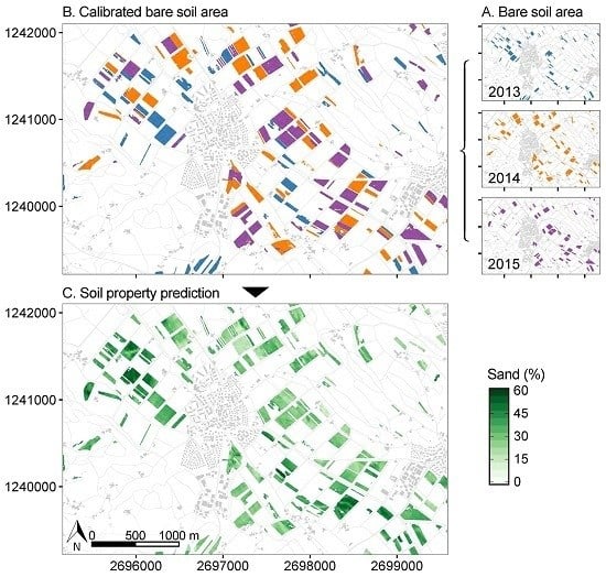
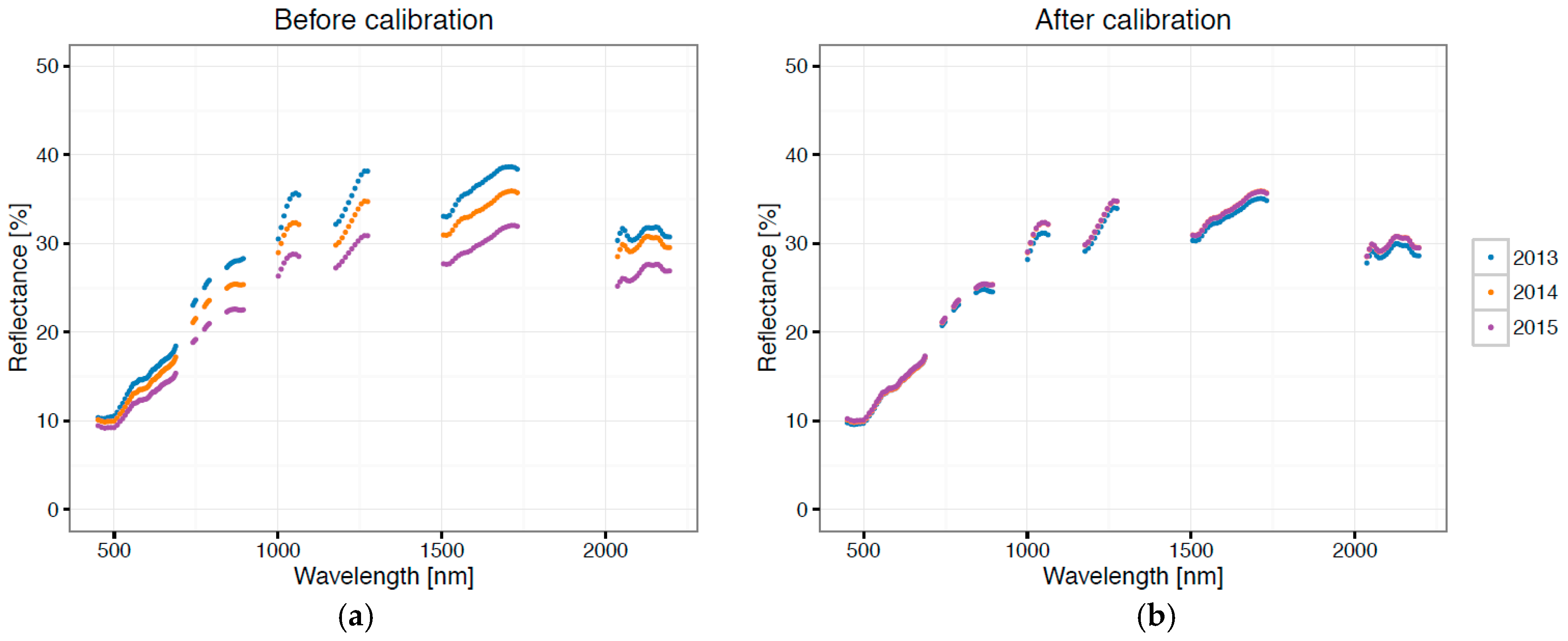
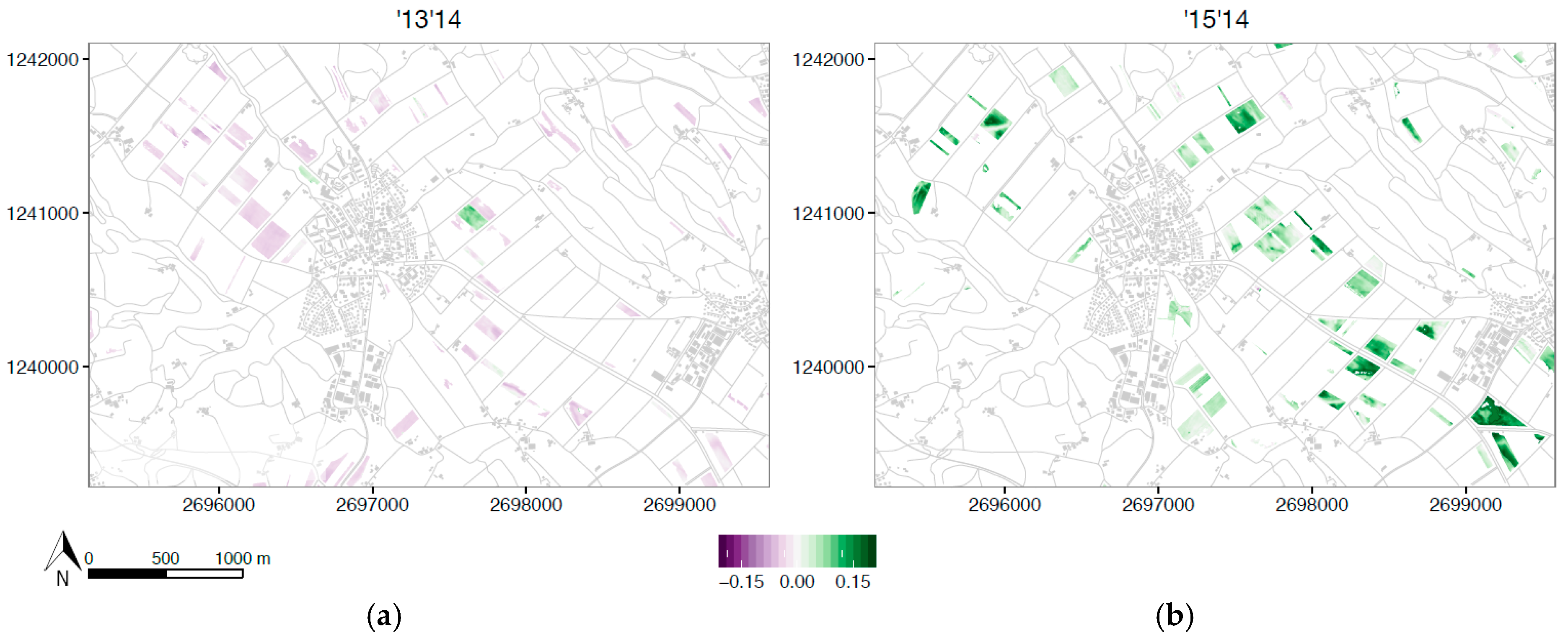
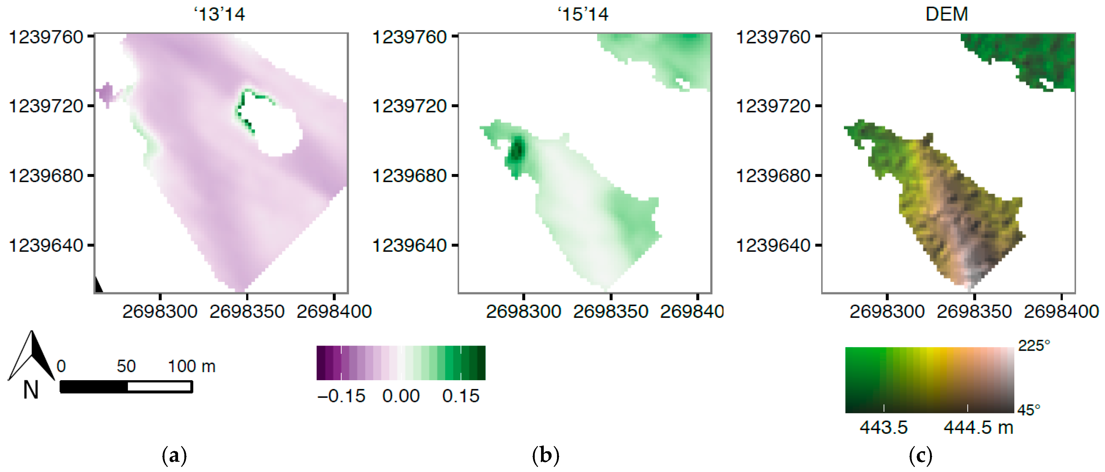
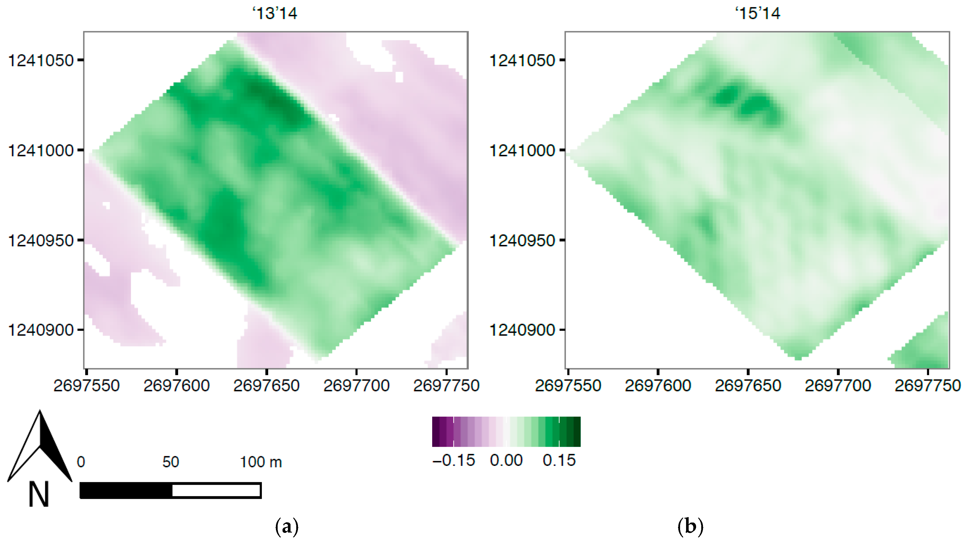
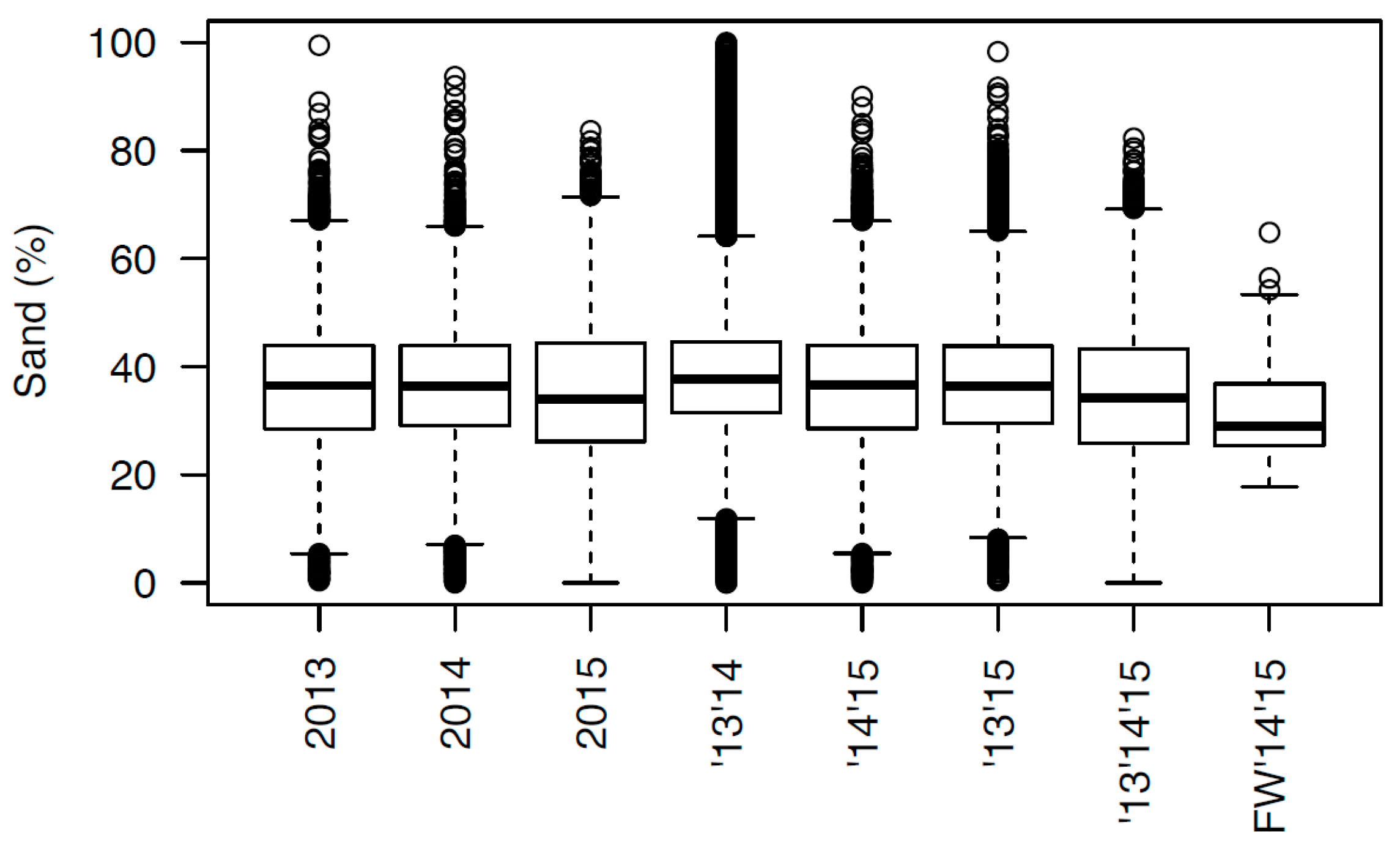
With this study, we have focused on one of the challenges of in-field soil spectroscopy in a temperate climate: soil surface coverage. The presence of crop rotation made it possible to select various bare soils in three subsequent years and has shown to be useful to increase observable bare soil area. Unlike previous studies using crop rotation to increase the bare soil area based on soil property derivations, we show that using the original spectroscopy data of multiple years, as opposed to compositing derived soil products, is successful. However, calibration is necessary to correct for differences in soil moisture and soil surface roughness as a result of changing weather and land management conditions. The difference indicators show that the calibration was successful (decrease in root mean square difference and angle difference, increase in R2 and gain and offset close to one and zero). Creating a multi-temporal composite of the calibrated imaging spectroscopy data has resulted in more than double the area (106.4%) of bare soils available in a single image. This composite image did not only show similar summary statistics compared to the reference image (mean and standard deviation of 2014: 24.2 ± 8.9 vs. 24.0 ± 9.5 for the multi-temporal composite ‘13’14’15), but also revealed the general long-term spatial pattern that is necessary for deriving soil properties at larger scales. Although global linear variability in short-term processes, such as variation in soil moisture and soil surface roughness, were accounted for, local non-linear variability in short-term processes could not be accounted for.
Naturally, this also means that there are still challenges to solve for in-field soil spectroscopy in temperate climates. Firstly, it is necessary to correct for the local non-linear short-term processes, which are causing variation in soil moisture and soil surface roughness. Unfortunately, only few studies focus on in-field measurements (e.g., [19]), and to our knowledge no study combines both the effect of soil moisture and soil surface roughness. Therefore, more research is necessary to remove both the effect of soil moisture and the effect of soil surface roughness on spectroscopy data. Secondly, in order to make remote sensing—and spectroscopy in particular—widely applicable and accepted within the soil science, it is necessary to further extent sparse bare soil observations to full-coverage maps [4]. This calls for sophisticated interpolation and even extrapolation methods that use all available a-priori information for a best prediction of soil parameters in covered areas [4]. Although some research has been done on this subject [9], the challenge remains to retain as much of the small scale variability that is offered by the spectroscopy data as possible. Increasing the bare soil area is possible by creating a multi-temporal composite, however, the question of how (spectral) information can be used to provide detailed information on soil properties in permanently covered areas remains. We are planning to make these challenges the focus of our follow-up papers.

Acknowledgments

This study was funded by the Swiss National Science Foundation (SNSF) in the frame of the National Research Programme “Sustainable use of Soil as a Resource” (NRP 68). Within the NRP 68, the study was part of the project “Predictive mapping of soil properties for the evaluation of soil functions at regional scale” (www.nfp68.ch). The contribution of M.E.S. is supported by the University of Zurich Research Priority Program on ‘Global Change and Biodiversity’ (URPP GCB). We thank RSL, MMRS and GIS staff supporting fieldwork. APEX data acquisition was supported by the Swiss Earth Observatory Network (http://www.seon.uzh.ch) project.

Author Contributions

S.D. designed the research and analyzed the data with scientific advice of R.d.J. and M.E.S. S.D. wrote the manuscript and all co-authors thoroughly reviewed and edited the manuscript.

Conflicts of Interest

The authors declare no conflict of interest. The founding sponsors had no role in the design of the study; in the collection, analyses, or interpretation of data; in the writing of the manuscript, and in the decision to publish the results.

Abbreviations

The following abbreviations are used in this manuscript:
APEXAirborne Prism EXperiment
DEMdigital elevation model
nCAInormalized cellulose absorption index
NDRBInormalized difference red blue index
NDVInormalized difference vegetation index
NIRnear-infrared
PCprincipal component
PCAprincipal component analysis
PLSRpartial least squares regression
SM(A)PEsymmetric mean (absolute) percentage error
SNRsignal to noise ratio
SWIRshort-wave infrared
VISvisible
VNIRvisible and near-infrared

Appendix A

Table A1. Relative difference (%) in mean reflectance before calibration.
Yearn 1ALL 2VIS 3NIR 4SWIR 5
‘13’1454,98111.7 ± 14.110.6 ± 14.113.8 ± 12.511.2 ± 15.1
‘15’14154,270−8.2 ± 14.0−8.7 ± 13.2−7.7 ± 14.7−8.0 ± 14.3
1 The number of overlapping pixels (excluding outliers according to Equations (3) and (4)); 2 Full spectrum 450–2200 nm; 3 Visible spectrum 450–700 nm; 4 Near-infrared spectrum 700–1400 nm; 5 Short-wave infrared 1400–2200 nm.

Appendix B

Figure B1. Distribution of the predicted sand percentages for all single images (2013, 2014, and 2015) and the multi-temporal composites (‘13’14, ‘14’15, ‘13’15, and ‘13’14’15) next to the distribution of the sand percentages of the field samples of ’14 and ’15.
Remotesensing 08 00906 g014

References

  1. Ben-Dor, E.; Irons, J.R.; Epema, G. Chapter 3: Soil Reflectance. In Remote Sensing for the Earth Sciences, 3rd ed.; Rencz, A.N., Ed.; John Wiley & Sons, Inc.: Hoboken, NJ, USA, 1999; pp. 111–188. [Google Scholar]
  2. Jenny, H. Factors of Soil Formation. A System of Quantitative Pedology, 1st ed.; McGraw-Hill Book Company, Inc.: New York, NY, USA, 1941; p. 281. [Google Scholar]
  3. Völkel, J.; Huber, J.; Leopold, M. Significance of slope sediments layering on physical characteristics and interflow within the Critical Zone—Examples from the Colorado Front Range, USA. Appl. Geochem. 2011, 26, S143–S145. [Google Scholar] [CrossRef]
  4. Mulder, V.L.; de Bruin, S.; Schaepman, M.E.; Mayr, T.R. The use of remote sensing in soil and terrain mapping—A review. Geoderma 2011, 162, 1–19. [Google Scholar] [CrossRef]
  5. Nocita, M.; Stevens, A.; van Wesemael, B.; Brown, D.J.; Shepherd, K.D.; Towett, E.; Vargas, R.; Montanarella, L. Soil spectroscopy: An opportunity to be seized. Glob. Ch. Biol. 2014. [Google Scholar] [CrossRef] [PubMed]
  6. Viscarra Rossel, R.A.; Cattle, S.R.; Ortega, A.; Fouad, Y. In situ measurements of soil colour, mineral composition and clay content by VIS-NIR spectroscopy. Geoderma 2009, 150, 253–266. [Google Scholar] [CrossRef]
  7. Viscarra Rossel, R.A.; Walvoort, D.J.J.; McBratney, A.B.; Janik, L.J.; Skjemstad, J.O. Visible, near infrared, mid infrared or combined diffuse reflectance spectroscopy for simultaneous assessment of various soil properties. Geoderma 2006, 131, 59–75. [Google Scholar] [CrossRef]
  8. Ben-Dor, E.; Chabrillat, S.; Demattê, J.A.M.; Taylor, G.R.; Hill, J.; Whiting, M.L.; Sommer, S. Using imaging spectroscopy to study soil properties. Remote Sens. Environ. 2009, 113, S38–S55. [Google Scholar] [CrossRef]
  9. Lagacherie, P.; Bailly, J.S.; Monestiez, P.; Gomez, C. Using scattered hyperspectral imagery data to map the soil properties of a region. Eur. J. Soil Sci. 2012, 63, 110–119. [Google Scholar] [CrossRef]
  10. Stevens, A.; Udelhoven, T.; Denis, A.; Tychon, B.; Lioy, R.; Hoffmann, L.; van Wesemael, B. Measuring soil organic carbon in croplands at regional scale using airborne imaging spectroscopy. Geoderma 2010, 158, 32–45. [Google Scholar] [CrossRef]
  11. Kokaly, R.F.; King, T.V.V.; Hoefen, T.M. Surface Mineral Maps of Afghanistan Derived From HyMap Imaging Spectrometer Data, Version 2; U.S. Geological Survey: Reston, VA, USA, 2013.
  12. Mulder, V.L.; Plötze, M.; de Bruin, S.; Schaepman, M.E.; Mavris, C.; Kokaly, R.F.; Egli, M. Quantifying mineral abundances of complex mixtures by coupling spectral deconvolution of SWIR spectra (2.1–2.4 µm) and regression tree analysis. Geoderma 2013, 207–208, 279–290. [Google Scholar] [CrossRef]
  13. Selige, T.; Böhner, J.; Schmidhalter, U. High resolution topsoil mapping using hyperspectral image and field data in multivariate regression modeling procedures. Geoderma 2006, 136, 235–244. [Google Scholar] [CrossRef]
  14. Bartholomeus, H.; Kooistra, L.; Stevens, A.; van Leeuwen, M.; van Wesemael, B.; Ben-Dor, E.; Tychon, B. Soil organic carbon mapping of partially vegetated agricultural fields with imaging spectroscopy. Int. J. Appl. Earth Obs. Geoinf. 2011, 13, 81–88. [Google Scholar] [CrossRef]
  15. Soriano-Disla, J.M.; Janik, L.J.; Viscarra Rossel, R.A.; MacDonald, L.M.; McLaughlin, M.J. The performance of visible, near-, and mid-infrared reflectance spectroscopy for prediction of soil physical, chemical, and biological properties. Appl. Spectrosc. Rev. 2014, 49, 139–186. [Google Scholar] [CrossRef]
  16. Udelhoven, T.; Emmerling, C.; Jarmer, T. Quantitative analysis of soil chemical properties with diffuse reflectance spectrometry and partial least-square regression: A feasibility study. Plant Soil 2003, 251, 319–329. [Google Scholar] [CrossRef]
  17. Gomez, C.; Viscarra Rossel, R.A.; McBratney, A.B. Soil organic carbon prediction by hyperspectral remote sensing and field VIS-NIR spectroscopy: An Australian case study. Geoderma 2008, 146, 403–411. [Google Scholar] [CrossRef]
  18. Stevens, A.; van Wesemael, B.; Bartholomeus, H.; Rosillon, D.; Tychon, B.; Ben-Dor, E. Laboratory, field and airborne spectroscopy for monitoring organic carbon content in agricultural soils. Geoderma 2008, 144, 395–404. [Google Scholar] [CrossRef]
  19. Denis, A.; Stevens, A.; van Wesemael, B.; Udelhoven, T.; Tychon, B. Soil organic carbon assessment by field and airborne spectrometry in bare croplands: Accounting for soil surface roughness. Geoderma 2014, 226–227, 94–102. [Google Scholar] [CrossRef]
  20. Wu, C.Y.; Jacobson, A.R.; Laba, M.; Baveye, P.C. Accounting for surface roughness effects in the near-infrared reflectance sensing of soils. Geoderma 2009, 152, 171–180. [Google Scholar] [CrossRef]
  21. Atzberger, C. Systematic Evaluation of Factors Interfearing with Soil Color Retrieval from Space. In Proceedings of the Second EARSeL Workshop on Imaging Spectroscopy, Enschede, The Netherlands, 11–13 July 2000.
  22. Gerighausen, H.; Menz, G.; Kaufmann, H. Spatially explicit estimation of clay and organic carbon content in agricultural soils using multi-annual imaging spectroscopy data. Appl. Environ. Soil Sci. 2012. [Google Scholar] [CrossRef]
  23. ESA. Sentinel-2. Available online: https://earth.esa.int/web/guest/missions/esa-operational-eo-missions/sentinel-2 (accessed on 12 September 2016).
  24. DLR. EnMAP Mission. Available online: http://www.enmap.org/?q=mission (accessed on 12 September 2016).
  25. Stefano, P.; Angelo, P.; Simone, P.; Filomena, R.; Federico, S.; Tiziana, S.; Umberto, A.; Vincenzo, C.; Acito, N.; Marco, D.; et al. The prisma hyperspectral mission: science activities and opportunities for agriculture and land monitoring. In Proceedings of the 2013 International Geoscience and Remote Sensing Symposium (IGARSS), Melbourne, Australia, 21–26 July 2013; pp. 4558–4561.
  26. Iwasaki, A.; Ohgi, N.; Tanii, J.; Kawashima, T.; Inada, H. Hyperspectral Imager Suite (HISUI)—Japanese hyper-multi spectral radiometer. In Proceedings of the 2011 International Geoscience and Remote Sensing Symposium (IGARSS), Vancouver, BC, Canada, 24–29 July 2011; pp. 1025–1028.
  27. ISA. The Shalom Mission. Available online: http://space.gov.il/en/node/1144 (accessed on 12 September 2016).
  28. NASA. HyspIRI Mission Study. Available online: https://hyspiri.jpl.nasa.gov/ (accessed on 12 September 2016).
  29. Nocita, M.; Stevens, A.; Noon, C.; Van Wesemael, B. Prediction of soil organic carbon for different levels of soil moisture using VIS-NIR spectroscopy. Geoderma 2013, 199, 37–42. [Google Scholar] [CrossRef]
  30. Wang, J.R.; O’Neill, P.E.; Jackson, T.J.; Engman, E.T. Multifrequency measurements of the effects of soil moisture, soil texture, and surface roughness. IEEE Trans. Geosci. Remote Sens. 1983, 21, 44–51. [Google Scholar] [CrossRef]
  31. Wang, Z.; Coburn, C.A.; Ren, X.; Teillet, P.M. Effect of soil surface roughness and scene components on soil surface bidirectional reflectance factor. Can. J. Soil Sci. 2012, 92, 297–313. [Google Scholar] [CrossRef]
  32. Cierniewski, J. A model for soil surface roughness influence on the spectral response of bare soils in the visible and near-infrared range. Remote Sens. Environ. 1987, 23, 97–115. [Google Scholar] [CrossRef]
  33. Piekarczyk, J.; Kazmierowski, C.; Krolewicz, S.; Cierniewski, J. Effects of soil surface roughness on soil reflectance measured in laboratory and outdoor conditions. IEEE J. Sel. Top. Appl. Earth Obs. Remote Sens. 2016, 9, 827–834. [Google Scholar] [CrossRef]
  34. Bogrekci, I.; Lee, W.S. Effects of soil moisture content on absorbance spectra of sandy soils in sensing phosphorus concentrations using UV-VIS-NIR spectroscopy. Trans. ASABE 2006, 49, 1175–1180. [Google Scholar] [CrossRef]
  35. Minasny, B.; McBratney, A.B.; Bellon-Maurel, V.; Roger, J.M.; Gobrecht, A.; Ferrand, L.; Joalland, S. Removing the effect of soil moisture from NIR diffuse reflectance spectra for the prediction of soil organic carbon. Geoderma 2011, 167–168, 118–124. [Google Scholar] [CrossRef]
  36. Castaldi, F.; Palombo, A.; Pascucci, S.; Pignatti, S.; Santini, F.; Casa, R. Reducing the influence of soil moisture on the estimation of clay from hyperspectral data: A case study using simulated PRISMA data. Remote Sens. 2015, 7, 15561–15582. [Google Scholar] [CrossRef]
  37. Levitt, D.G.; Simpson, J.R.; Huete, A.R. Estimates of surface soil water content using linear combinations of spectral wavebands. Theor. Appl. Climatol. 1990, 42, 245–252. [Google Scholar] [CrossRef]
  38. Haubrock, S.N.; Chabrillat, S.; Kuhnert, M.; Hostert, P.; Kaufmann, H. Surface soil moisture quantification and validation based on hyperspectral data and field measurements. J. Appl. Remote Sens. 2008. [Google Scholar] [CrossRef]
  39. Baumgardner, M.F.; Silva, L.F.; Biehl, L.L.; Stoner, E.R. Reflectance properties of soils. Adv. Agron. 1985, 38, 1–44. [Google Scholar]
  40. Bowers, S.A.; Hanks, R.J. Reflection of radiant energy from soils. Soil Sci. 1965, 100, 130–138. [Google Scholar] [CrossRef]
  41. Bolliger, T.; Gatti, H.; Hantke, R. Zur Geologie und Paläontologie des Zürcher Oberlandes. Vierteljahrsschrift der Naturforschenden Gesellschaft in Zürich 1988, 133, 1–24. [Google Scholar]
  42. Amt für Landschaft und Natur. Bodenkarte Kanton Zürich 1:5000; Amt für Landschaft und Natur: Zürich, Swizerland, 1998. [Google Scholar]
  43. Fachstelle Bodenschutz. Bodenkartierung der Landwirtschaftsflächen des Kantons Zürich: Erläuterungen und Glossar; Fachstelle Bodenschutz: Zürich, Swizerland, 2016. [Google Scholar]
  44. Jäggli, F.; Peyer, K.; Pazeller, A.; Schwab, P. Grundlagenbericht zur Bodenkartierung des Kantons Zürich; Eidgenössische Forschungsanstalt für Agrarökologie und Landbau (FAL), Volkwirtschaftdirektion des: Zürich, Switzerland, 1998. [Google Scholar]
  45. IUSS Working Group WRB. World Reference Base for Soil Resources 2006, First Update 2007; FAO: Rome, Italy, 2007. [Google Scholar]
  46. Bundesamt für Landestopografie Swisstopo. SwissTLM3D; Bundesamt für Landestopografie Swisstopo: Wabern, Switzerland, 2014. [Google Scholar]
  47. Franzen, J.; Müller, M.; Keller, A. Stoffbilanzen für Parzellen der Nationalen Bodenbeobachtung-Nähr-und Schadstoffe 1985–2014. 2016; in prepration. [Google Scholar]
  48. Schaepman, M.E.; Jehle, M.; Hueni, A.; D’Odorico, P.; Damm, A.; Weyermann, J.; Schneider, F.D.; Laurent, V.; Popp, C.; Seidel, F.C.; et al. Advanced radiometry measurements and Earth science applications with the Airborne Prism Experiment (APEX). Remote Sens. Environ. 2015, 158, 207–219. [Google Scholar] [CrossRef]
  49. Hueni, A.; Lenhard, K.; Baumgartner, A.; Schaepman, M.E. Airborne Prism Experiment calibration information system. IEEE Trans. Geosci. Remote Sens. 2013. [Google Scholar] [CrossRef] [Green Version]
  50. Jehle, M.; Hueni, A.; Damm, A.; D’Odorico, P.; Weyermann, J.; Kneubühler, M.; Schläpfer, D.; Schaepman, M.E.; Meuleman, K. APEX-Current Status, Performance and Validation Concept. In Proceedings of the 2010 IEEE Sensors Conference, Waikoloa, HI, USA, 1–4 November 2010.
  51. Hueni, A.; Biesemans, J.; Meuleman, K.; Dell’Endice, F.; Schläpfer, D.; Odermatt, D.; Kneubühler, M.; Adriaensen, S.; Kempenaers, S.; Nieke, J.; et al. Structure, components, and interfaces of the airborne prism experiment (APEX) processing and archiving facility. IEEE Trans. Geosci. Remote Sens. 2009, 47, 29–43. [Google Scholar] [CrossRef] [Green Version]
  52. Rouse, J.W., Jr.; Haas, R.H.; Schell, J.A.; Deering, D.W. Monitoring vegetation systems in the Great Plains with ERTS. In Proceedings of the Third ERTS Symposium, Washington, DC, USA, 10–14 December 1973.
  53. Tucker, C.J. Red and photographic infrared linear combinations for monitoring vegetation. Remote Sens. Environ. 1979, 8, 127–150. [Google Scholar] [CrossRef]
  54. Carter, G.A. Primary and secondary effects on water content on the spectral reflectance of leaves. Am. J. Bot. 1991, 78, 916–924. [Google Scholar] [CrossRef]
  55. Zakaluk, R.; Sri Ranjan, R. Predicting the leaf water potential of potato plants using RGB reflectance. Can. Biosyst. Eng. 2008, 50, 7.1–7.12. [Google Scholar]
  56. Nagler, P.L.; Inoue, Y.; Glenn, E.P.; Russ, A.L.; Daughtry, C.S.T. Cellulose absorption index (CAI) to quantify mixed soil-plant litter scenes. Remote Sens. Environ. 2003, 87, 310–325. [Google Scholar] [CrossRef]
  57. Chabrillat, S.; Eisele, A.; Guillaso, S.; Rogaß, C.; Ben-Dor, E.; Kaufmann, H. HYSOMA: An easy-to-use software interface for soil mapping applications of hyperspectral imagery. In Proceedings of the 7th EARSeL SIG Imaging Spectroscopy Workshop, Edinburgh, UK, 11–13 April 2011.
  58. Bundesamt für Landwirtschaft. Feldblockkarte Zum Erosionsrisiko; Bundesamt für Landwirtschaft: Bern, Switzerland, 2014. [Google Scholar]
  59. Bundesamt für Landestopografie Swisstopo. SwissBUILDINGS3D 1.0; Bundesamt für Landestopografie Swisstopo: Wabern, Switzerland, 2014. [Google Scholar]
  60. Conel, J.E.; Green, R.O.; Vane, G.; Bruegge, C.J.; Alley, R.E. AIS-2 Radiometry and a Comparison of Methods for the Recovery of Ground Reflectance. In Proceedings of the 3rd Airborne Imaging Spectrometer Data Analysis Workshop, Pasadena, CA, USA, 2–4 June 1987.
  61. Smith, G.M.; Milton, E.J. The use of the empirical line method to calibrate remotely sensed data to reflectance. Int. J. Remote Sens. 1999, 20, 2653–2662. [Google Scholar] [CrossRef]
  62. Kruse, F.A.; Kierein-Young, K.S.; Boardman, J.W. Mineral mapping at Cuprite, Nevada with a 63-channel imaging spectrometer. Photogram. Eng. Remote Sens. 1990, 56, 83–92. [Google Scholar]
  63. Cook, R.D.; Weisberg, S. Residuals and Influence in Regression; Chapman and Hall: New York, NY, USA, 1982. [Google Scholar]
  64. Bollen, K.A.; Jackman, R.W. Regression diagnostics: An expository treatment of outliers and influential cases. In Modern Methods of Data Analysis; Fox, J., Long, J.S., Eds.; Sage: Newbury Park, CA, USA, 1990; pp. 257–291. [Google Scholar]
  65. Price, J.C. How unique are spectral signatures? Remote Sens. Environ. 1994, 49, 181–186. [Google Scholar] [CrossRef]
  66. Breunig, F.M.; Galvão, L.S.; Formaggio, A.R. Detection of sandy soil surfaces using ASTER-derived reflectance, emissivity and elevation data: Potential for the identification of land degradation. Int. J. Remote Sens. 2008, 29, 1833–1840. [Google Scholar] [CrossRef]
  67. Chabrillat, S.; Goetz, A.F.H.; Krosley, L.; Olsen, H.W. Use of hyperspectral images in the identification and mapping of expansive clay soils and the role of spatial resolution. Remote Sens. Environ. 2002, 82, 431–445. [Google Scholar] [CrossRef]
  68. Bartholomeus, H.M.; Schaepman, M.E.; Kooistra, L.; Stevens, A.; Hoogmoed, W.B.; Spaargaren, O.S.P. Spectral reflectance based indices for soil organic carbon quantification. Geoderma 2008, 145, 28–36. [Google Scholar] [CrossRef]
  69. Flores, B.E. A pragmatic view of accuracy measurement in forecasting. Omega 1986, 14, 93–98. [Google Scholar] [CrossRef]
  70. Hotelling, H. Analysis of a complex of statistical variables into principal components. J. Educ. Psychol. 1933, 24, 498–520. [Google Scholar] [CrossRef]
  71. Pearson, K. On lines and planes of closest fit to systems of points in space. Philos. Mag. 1901, 2, 559–572. [Google Scholar] [CrossRef]
  72. James, G.; Witten, D.; Hastie, T.; Tibshirani, R. An Introduction to Statistical Learning with Applications in R; Springer: New York, NY, USA, 2015. [Google Scholar]
  73. McBratney, A.B.; Mendonça Santos, M.L.; Minasny, B. On digital soil mapping. Geoderma 2003, 117, 3–52. [Google Scholar] [CrossRef]
  74. Haaland, D.M.; Thomas, E.V. Partial least-squares methods for spectral analyses. 1. Relation to other quantitative calibration methods and the extraction of qualitative information. Anal. Chem. 1988, 60, 1193–1202. [Google Scholar] [CrossRef]
  75. R Core Team. R: A Language and Environment for Statistical Computing. Available online: https://www.R-project.org/ (accessed on 12 September 2016).
  76. Cressie, N.A.C. Statistics for Spatial Data; John Wiley & Sons: London, UK, 1993; p. 928. [Google Scholar]
  77. Ettema, C.H.; Wardle, D.A. Spatial soil ecology. Trends Ecol. Evol. 2002, 17, 177–183. [Google Scholar] [CrossRef]
  78. Pebesma, E.J. Multivariable geostatistics in S: The gstat package. Comput. Geosci. 2004, 30, 683–691. [Google Scholar] [CrossRef]
  79. Pebesma, E.J.; Wesseling, C.G. Gstat, a program for geostatistical modelling, prediction and simulation. Comput. Geosci. 1998, 24, 17–31. [Google Scholar] [CrossRef]
  80. Wold, H. Nonlinear estimation by iterative least square procedures. In Research Papers in Statistics; David, F.N., Ed.; John Wiley and Sons, Inc.: New York, NY, USA, 1966; pp. 411–444. [Google Scholar]
  81. Thomas, E.V.; Haaland, D.M. Comparison of multivariate calibration methods for quantitative spectral analysis. Anal. Chem. 1990, 62, 1091–1099. [Google Scholar] [CrossRef]
  82. Paz-Kagan, T.; Zaady, E.; Salbach, C.; Schmidt, A.; Lausch, A.; Zacharias, S.; Notesco, G.; Ben-Dor, E.; Karnieli, A. Mapping the Spectral Soil Quality Index (SSQI) using airborne imaging spectroscopy. Remote Sens. 2015, 7, 15748–15781. [Google Scholar] [CrossRef]
  83. Savitzky, A.; Golay, M.J.E. Smoothing and differentiation of data by simplified least squares procedures. Anal. Chem. 1964, 36, 1627–1639. [Google Scholar] [CrossRef]
  84. Fystro, G. The prediction of C and N content and their potential mineralisation in heterogeneous soil samples using VIS-NIR spectroscopy and comparative methods. Plant Soil 2002, 246, 139–149. [Google Scholar] [CrossRef]
Figure 1. Study area and the distribution of the bare soil pixels, the colors show in which year(s) the considering bare soil pixel was present. The black rectangles show the locations of the focus area (used in most of the following figures) and the locations of the individual fields in Figure 7, Figure 8, Figure 9 and Figure 10.
Remotesensing 08 00906 g001
Figure 2. Precipitation (l·m−2) and temperature data (°C) in the 28 days before the flight dates (3 September 2013, 11 April 2014 and 10 April 2015).
Remotesensing 08 00906 g002
Figure 3. (ac) RGB-image of the focus area of the spectroscopy data for all flight dates (3 September 2013, 11 April 2014 and 10 April 2015); and (df) the corresponding selected bare soils for all three years.
Remotesensing 08 00906 g003
Figure 4. Mean reflectance values for all three years (2013, 2014, and 2015): before (a); and after (b) calibration.
Remotesensing 08 00906 g004
Figure 5. Distribution of the SMPE values for: (a) ‘13’14; and (b) ‘15’14. Distribution is given for the full spectra (ALL: 450–2200 nm), and for the specific ranges of the spectra (VIS: visible spectrum 450–700 nm, NIR: near-infrared spectrum 700–1400 nm, and SWIR: short-wave infrared 1400–2200 nm).
Remotesensing 08 00906 g005
Figure 6. Spatial distribution in the focus area of the SMPE values for: (a) ‘13’14; and (b) ‘15’14.
Remotesensing 08 00906 g006
Figure 7. SMPE values for: ‘13’14 (a); and ‘15’14 (b); and DEM (overlaid with a hillshade: 315° azimuth and 45° altitude) for an individual agricultural field (c).
Remotesensing 08 00906 g007
Figure 8. SMPE values for: ‘13’14 (a); and ‘15’14 (b) for an individual agricultural.
Remotesensing 08 00906 g008
Figure 9. Close-up of an individual agricultural field showing the year(s) each bare soil pixel was present (a); and the first PC of the multi-temporal composite (b).
Remotesensing 08 00906 g009
Figure 10. The first PC values (df,km); the corresponding 45° and 315° variograms (ac,hj); and the DEM (overlaid with a hillshade: 315° azimuth and 45° altitude) of two individual agricultural fields (Field I and Field II) for all three years (2013, 2014, and 2015) (g,n). The axes of the variograms have the distance (m) on the x-axis and the semi-variance on the y-axis.
Remotesensing 08 00906 g010
Figure 11. In-field variability shown by the first PC values: (ac) for an individual agricultural field for all three years (2013, 2014, and 2015); and the corresponding DEM (overlaid with a hillshade: 315° azimuth and 45° altitude) (d).
Remotesensing 08 00906 g011
Figure 12. The 45° and 315° variograms at long distances for the first PC values (ag) for all single (2013, 2014, and 2015) and multi-temporal composites (‘13’14, ‘14’15, ‘13’15, and ‘13’14’15). On the x-axis the distance (m) and on the y-axis the semi-variance.
Remotesensing 08 00906 g012
Figure 13. The 45° and 315° variograms at short distances for the first PC values (ag) for all single (2013, 2014, and 2015) and multi-temporal composites (‘13’14, ‘14’15, ‘13’15, and ‘13’14’15). On the x-axis the distance [m] and on the y-axis the semi-variance.
Remotesensing 08 00906 g013
Table 1. Sowing and harvest periods for the dominant crops (winter cereals, maize, and rapeseed) in the study area.
Jan. Feb.Mar.Apr. 1MayJun.Jul.Aug.Sep. 1Oct.Nov.Dec.
Barley winter
Triticale winter
Wheat winter
Rye winter
Spelt
Maize corn
Maize silage 2
Rapeseed
Green is sowing period, while blue is the harvesting period. Information is based on Franzen et al. [47]. 1 The black vertical lines indicate approximately the date of the flights (3 September 2013, 11 April 2014, 10 April 2015); 2 The light green for Maize silage indicates late sowing to grow green silage maize.
Table 2. Total number of bare soil pixels and the amount of overlapping pixels for the years 2013, 2014, and 2015.
YearNo. PixelsNo. Overlapping Pixels
2013536,213 1 (1.4% 2|2.9% 3)63,066 1
2014814,240 1 (2.1% 2|4.4% 3)
178,075 1
2015634,013 1 (1.6% 2|3.4% 3)
1 The total area in m2 can be calculated by multiplying the number of pixels with the area of 4 m2 per pixel (2 × 2 m); 2 Percentages show the coverage of the total study area (39,564,161 pixels) by bare soil; 3 Percentages show the coverage of the total agricultural area (18,647,218 pixels) by bare soil. The agricultural area was calculated based on the agricultural field block map [58].
Table 3. Difference (%) in mean reflectance before calibration.
Yearn 1ALL 2VIS 3NIR 4SWIR 5
‘13’1454,9812.57 ± 3.421.32 ± 1.943.64 ± 3.143.09 ± 4.31
‘15’14154,270−2.23 ± 3.77−1.34 ± 1.95−2.48 ± 4.27−2.97 ± 4.56
1 The number of overlapping pixels (excluding outliers according to Equations (3) and (4)); 2 Full spectrum 450–2200 nm; 3 Visible spectrum 450–700 nm; 4 Near-infrared spectrum 700–1400 nm; 5 Short-wave infrared 1400–2200 nm.
Table 4. Difference indicators and linear correlation results before calibration.
Yearn 1D 2θ 3R2 4Offset 4Gain 4
‘13’1454,9810.33 ± 0.170.05 ± 0.030.97 ± 0.03−0.29 ± 2.251.13 ± 0.16
‘15’14154,2700.34 ± 0.180.05 ± 0.030.98 ± 0.040.07 ± 2.010.92 ± 0.17
1 The number of overlapping pixels (excluding outliers according to Equations (3) and (4)); 2 The square difference as defined in Equation (5); 3 The difference angle as defined in Equation (6); 4 R2, gain and offset calculated according to the linear correlation between the calibration year and the reference year (2014), following Equation (7).
Table 5. Difference (%) in mean reflectance after calibration.
Yearn 1ALL 2VIS 3NIR 4SWIR 5
‘13’1454,9810.02 ± 3.040.02 ± 1.810.07 ± 2.95−0.03 ± 3.98
‘15’14154,270−0.04 ± 3.34−0.01 ± 1.77−0.02 ± 3.72−0.09 ± 4.19
1 The number of overlapping pixels (excluding outliers according to Equations (3) and (4)); 2 Full spectrum 450–2200 nm; 3 Visible spectrum 450–700 nm; 4 Near-infrared spectrum 700–1400 nm; 5 Short-wave infrared 1400–2200 nm.
Table 6. Difference indicators and linear correlation results after calibration.
Yearn 1D 2θ 3R2 4Offset 4Gain 4
‘13’1454,9810.22 ± 0.140.04 ± 0.020.98 ± 0.030.07 ± 2.061.01 ± 0.15
‘15’14154,2700.25 ± 0.150.04 ± 0.030.98 ± 0.030.19 ± 2.001.01 ± 0.17
1 The number of overlapping pixels (excluding outliers according to Equations (3) and (4)); 2 The square difference as defined in Equation (5); 3 The difference angle as defined in Equation (6); 4 R2, gain and offset calculated according to the linear correlation between the calibration year and the reference year (2014), following Equation (7).
Table 7. Total number of bare soil pixels and the corresponding increase compared to 2014 (814,240 pixels is equal to 100%) for the multi-temporal composites ‘13’14, ‘14’15, ‘13’15, and ‘13’14’15.
YearNo. PixelsIncrease (2014 = 100%)
‘13’141,287,387 1 (3.3% 2|6.9% 3)158.1%
‘14’151,270,178 1 (3.2% 2|6.8% 3)156.0%
‘13’151,082,639 1 (2.7% 2|5.8% 3)132.9%
‘13’14’151,680,799 1 (4.2% 2|9.0% 3)206.4%
1 The total area in m2 can be calculated by multiplying the number of pixels with the area of 4 m2 per pixel (2 × 2 m); 2 Percentages show the coverage of the total study area (39,564,161 pixels) by bare soil; 3 Percentages show the coverage of the total agricultural area (18,647,218 pixels) by bare soil. The agricultural area was calculated based on the agricultural field block map [58].
Table 8. Mean and standard deviation of the reflectance values for the individual and multi-temporal images.
YearALL 1VIS 2NIR 3SWIR 4
201326.0 ± 9.914.9 ± 5.331.0 ± 7.634.1 ± 6.1
201424.2 ± 8.913.9 ± 3.728.4 ± 6.732.0 ± 6.3
201521.7 ± 8.912.6 ± 3.725.4 ± 6.528.5 ± 5.7
‘13’1424.0 ± 9.613.8 ± 3.828.1 ± 6.531.8 ± 5.5
‘14’1524.1 ± 9.613.9 ± 3.528.3 ± 6.231.9 ± 5.5
‘13’1524.0 ± 9.114.0 ± 3.528.2 ± 5.531.7 ± 3.7
‘13’14’1524.0 ± 9.513.9 ± 3.728.1 ± 6.231.8 ± 5.1
1 Full spectrum (450–2200 nm); 2 Visible spectrum ranging from 450–700 nm; 3 Near-infrared spectrum ranging from 700–1400 nm; 4 Short-wave infrared ranging from 1400–2200 nm.
Table 9. Sill and range values for the small-scale variogram for the agricultural field I and II (Figure 9).
YearField IField II
SillRangeSillRange
20138.369.531.3685.6
201411.763.88.249.3
20152.854.913.6128.9
Table 10. Sill and range values for the large-scale variograms at short (750 m) and long (5000 m) distance (Figure 12 and Figure 13).
YearLong Distance Short Distance
SillRangeSillRange
201387.5312.964.295.1
2014108.5317.8100.7222.5
2015113.2358.195.2194.4
‘13’14100.6266.598.0195.6
‘14’15112.5275.3106.6189.4
‘13’1586.9291.972.7134.0
‘13’14’15101.6234.599.2170.2
Table 11. Summary statistics (mean and standard deviation) for the measured soil properties.
Sand (%)Silt (%)Clay (%)OM 1 (%)SM 2 (%)SMupper 3 (%)
32.3 ± 10.038.2 ± 7.729.5 ± 11.410.3 ± 4.524.3 ± 7.62.6 ± 2.4
1 Organic matter; 2 Soil Moisture in the topsoil (upper 5 cm); 3 Soil Moisture upper topsoil (upper 1 cm).
Table 12. Partial least squares regression models and their performance.
YearNo. of Samples 1No. of PCs 2R 3 ± sd
‘131260.55 ± 0.16
‘144160.63 ± 0.03
‘157360.63 ± 0.02
‘13’145170.61 ± 0.03
‘14’158070.57 ± 0.02
‘13’157560.63 ± 0.02
‘13’14’158170.58 ± 0.02
1 The results of the intersection between the field samples and the spectral bare soil information; 2 The amount of PCs selected to make the soil property prediction; 3 The corresponding prediction R2 and its standard deviation calculated based on the bootstrapping results.
Table 13. Summary statistics of the results of predicted sand percentages of the overlapping bare soil pixels in all three years and of the sand percentages of the field samples (last row).
Yearn 1NAs 2Mean ± sd (%) 3Median (%)IQR (%) 4Min–Max (%)
‘13250616235.7 ± 11.636.628.5–44.00.4–99.5
‘142506110135.7 ± 11.536.429.1–43.90.0–93.7
‘152506110935.0 ± 11.934.026.2–44.40.0–83.7
‘13’142506135239.3 ± 12.737.731.5–44.60.0–100.0
‘14’15250615935.7 ± 11.636.628.6–44.00.1–90.0
‘13’1525061736.3 ± 11.536.429.6–43.80.4–98.3
‘13’14’152506115234.6 ± 12.434.225.9–43.30.0–82.3
FW’14’1589032.3 ± 10.029.125.4–36.917.8–64.9
1 The number of overlapping pixels; 2 The number of pixels excluded because the predicted values were below 0 or above 100; 3 The mean and its corresponding standard deviation; 4 The interquartile range.

