
Wind Turbine Wake Characterization from Temporally Disjunct 3-D Measurements

 , , and
Abstract
:
1. Introduction
2. Materials and Methods
2.1. Field Scans
- Data are filtered by range gate number (G), signal-to-noise ratio () and radial velocity magnitude (). The criteria are:and therefore, the total possible number of radial velocity measurements within a stack of scans is (number of gates ). The first range gate is discarded as it is in the LiDAR blind zone. The lower limit is recommended by the manufacturer, and the upper limit (also used in previous studies [16]) is enough to filter out hard targets and cloud water for our dataset. The upper limit in the radial velocities is an arbitrary value higher than any of the observed values during the measurement period (e.g., Figure 1) and serves to filter out unrealistic measurements and erroneous logging.
- The location vector in Cartesian coordinates in a fixed frame of reference for each point is obtained as:where () is positive in the east (north) direction. All quantities in the fixed frame are subscripted with F.
- For each 3D scanned volume, the highest elevation sector scan () is selected to determine the mean wind direction (angled brackets refer to values averaged over the entire 3D scan). Within this scan, all points sampled at least 0.25 D above the rotor are considered, which includes five range gates. An estimate of the horizontal wind components and is obtained for each range gate within this sector scan sub-sample by solving the linear system:using a least-squares approach, where () are the wind components along the directions () and are the radial velocity measurements along an arc of constant G for an azimuth angle . The vertical component is assumed to be negligible, consistent with previous studies (e.g., [23]). The validity of this assumption was verified with sonic anemometer data (not shown) and is based on the physical understanding that the magnitude of vertical velocities is much lower than that of horizontal velocities and that the mean magnitude of w is close to zero when averaged over periods of ∼10 min, which is approximately the time the LiDAR took to complete a full stack of sector scans. As suggested in [4], multiple LiDARs must be considered when seeking to investigate all components of the wind field within wakes.The values of () are then averaged across the five range gates within the sub-sample to yield the mean wind direction estimate for the scanned volume. The robustness of this method for the present experiment is reflected in the time series shown in Figure 3, where the minimum and maximum estimates for each 3D scan are compared with sonic anemometer measurements and the turbine nacelle position. The LiDAR estimates follow the sonic values more closely than the turbine data, indicating that the assumptions of low veer and negligible vertical velocity are acceptable for the atmospheric conditions observed during the experiment.
- Assuming a constant mean wind direction for each 3D scan, the horizontal wind speed at each point is estimated from the radial velocity as:where is the scan offset, defined as the angle between the scan wind direction and the laser beam azimuthal direction. Orthogonal scans are filtered out following the LiDAR manufacturer recommendation to remove points for which the laser beam makes an angle between and with the mean wind direction (∼1.4% of the measurements).
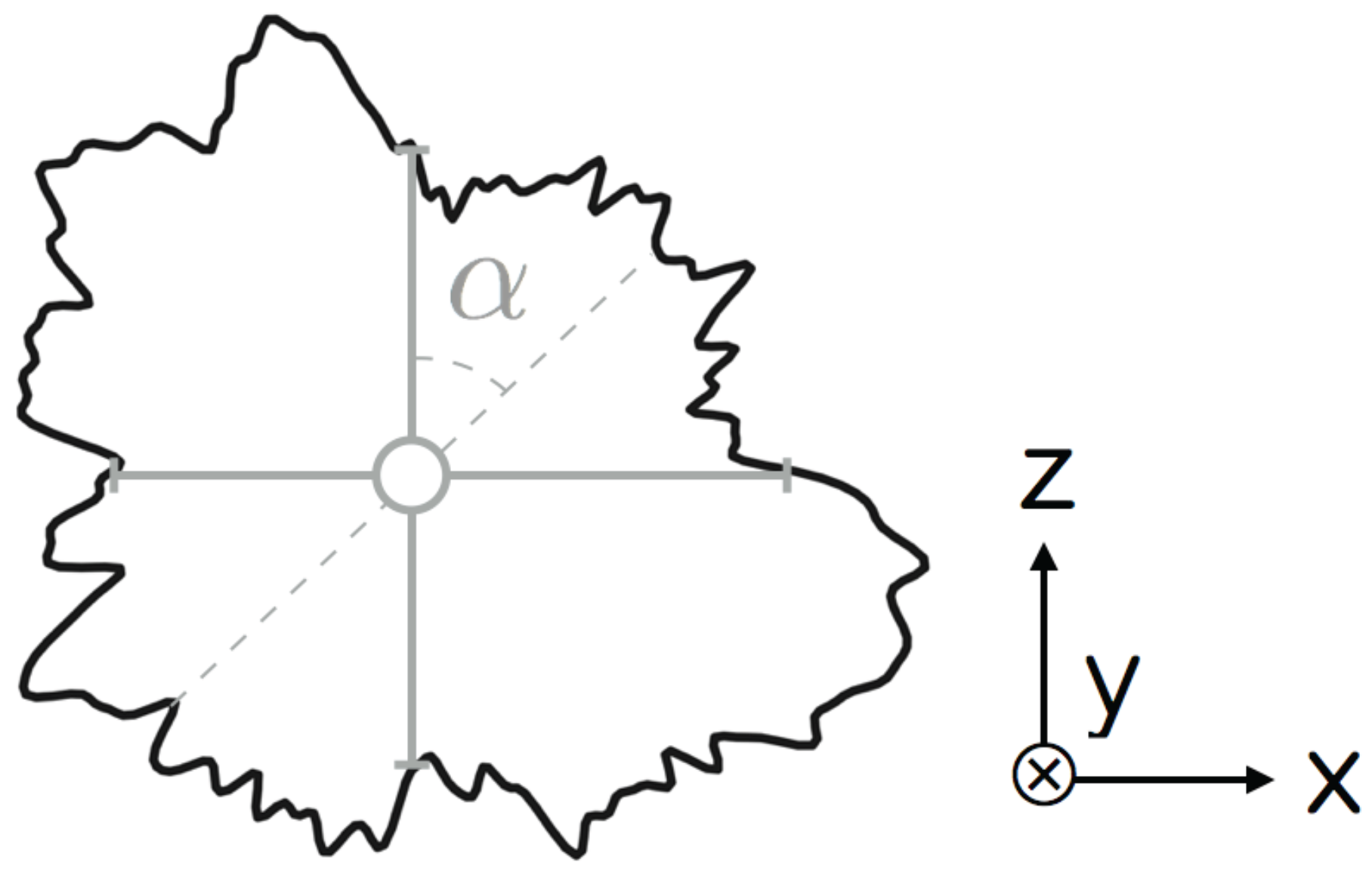
- All points in the scan are rotated so that the coordinate system is aligned with the mean wind direction. Throughout the manuscript, the quantities in this streamwise frame of reference are given without the F subscript as: , where x and y are the cross-stream and streamwise directions, respectively.
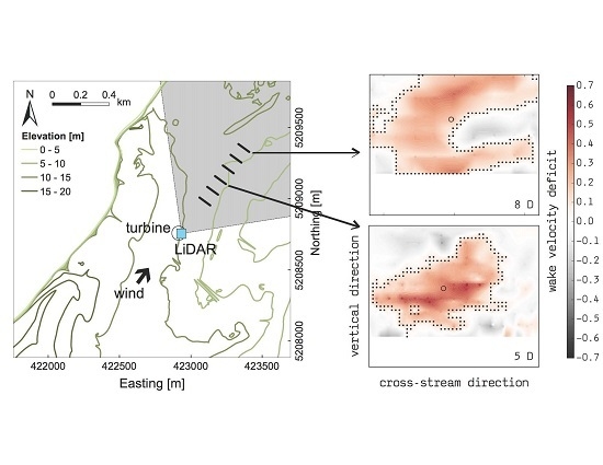
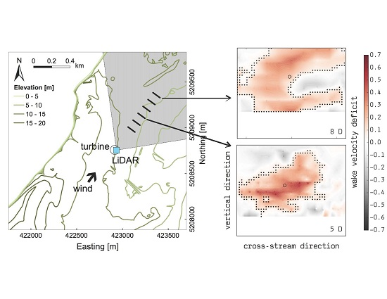
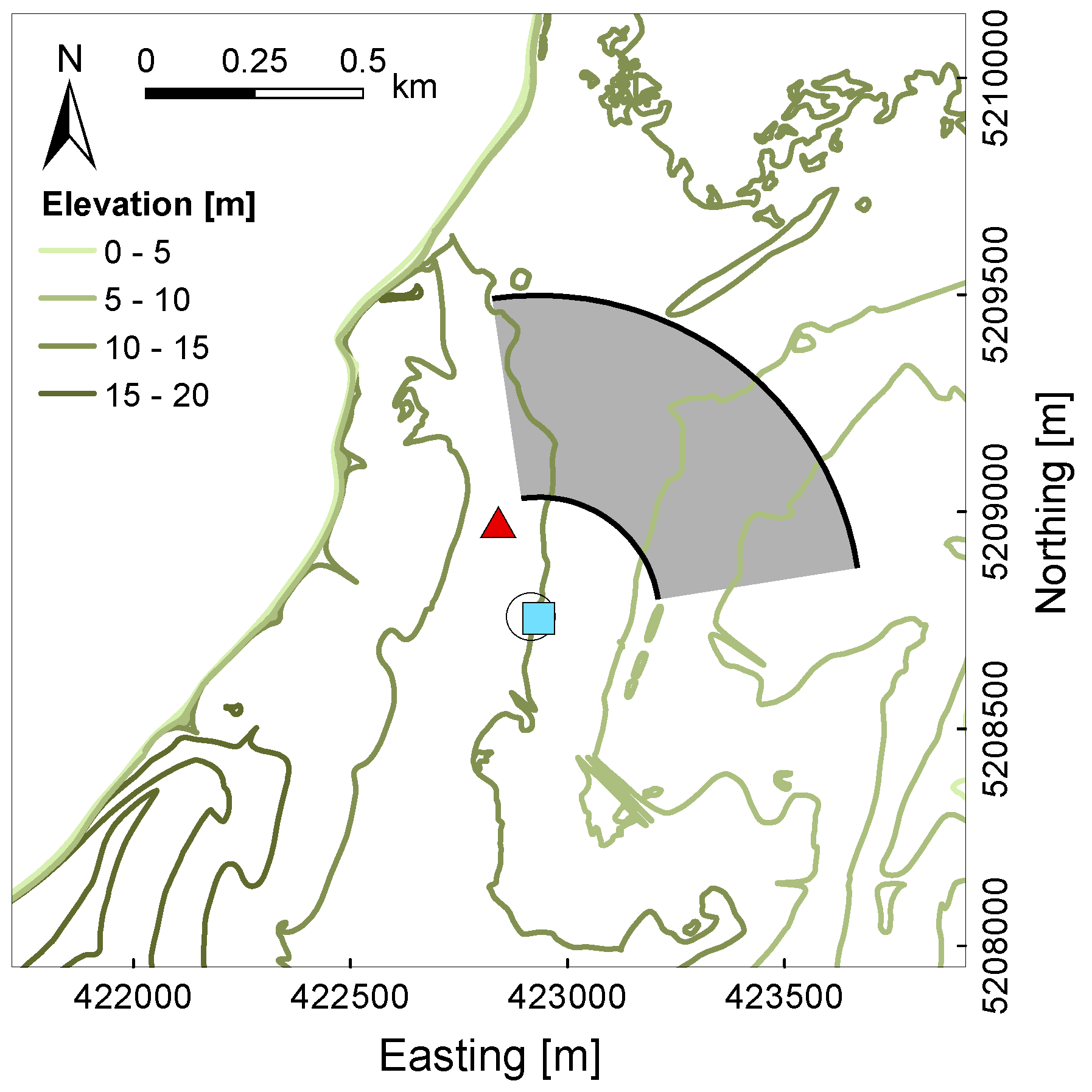
- Vertical planes of data are obtained at a given distance downstream of the turbine by selecting all of the sampled points whose streamwise coordinate y falls within the desired distance plus or minus some specified buffer , taken to be the range gate width of 30 m. In this analysis, the scanning LiDAR was deployed at the base of the turbine (Figure 2), and we apply an assumption of no yaw error. Therefore, the analysis only considers 3D scans for which the LiDAR-estimated is within of the turbine nacelle position, resulting in 80 sector scan stacks. The value of was chosen as a threshold because while it is small (half of the wind industry standard sectors when performing azimuthal analyses), it still allows for an offset between the turbine and the nacelle, which is necessary given the uncertainties inherent in both datasets (e.g., inaccuracies in the wind direction estimate from the LiDAR and in the recorded nacelle position) and the potential presence of yaw misalignment. As indicated by the sonic time series (Figure 3), the large differences between the LiDAR and the nacelle datasets reflect not an inability of the LiDAR to estimate the wind direction, but rather the necessarily delayed response of the nacelle to wind direction changes or high uncertainty in the turbine measurements.
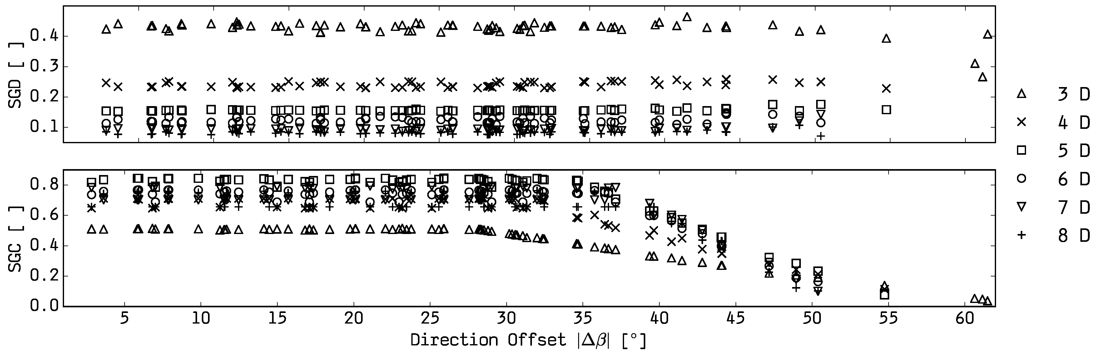
- In order to quantify the potential contribution of each vertical slice to wind turbine wake characterization, it is important to consider how much of the area of interest is covered by the sampled points and how dense this coverage is. To do that, we define two indices. The first one is the scanning geometry coverage (), which is calculated as:where A is the area covered by the scanned points within the total reference area , which extends 1 D to either side of the hub in the horizontal and vertical directions being only limited by the presence of the ground. Within the covered area A, the scanning geometry density () is defined as:where n is the number of points in the covered area A relative to a reference value , which is the maximum number of points that could cover the same area A given a desired fixed spatial resolution and , which for the present study is set to 5 m.
2.2. Synthetic Scans
2.3. Wake Identification
2.4. Wake Characterization
3. Results
3.1. Difference between Scan, Mean and Snapshot
3.2. Difference between Wake Characteristics from Scan, Mean and Snapshot
3.3. Field Wakes’ Characterization
4. Conclusions
Acknowledgments
Author Contributions
Conflicts of Interest
References
- Barthelmie, R.J.; Hansen, K.S.; Pryor, S.C. Meteorological Controls on Wind Turbine Wakes. Proc. IEEE 2013, 101, 1010–1019. [Google Scholar] [CrossRef]
- Käsler, Y.; Rahm, S.; Simmet, R.; Kühn, M. Wake Measurements of a Multi-MW Wind Turbine with Coherent Long-Range Pulsed Doppler Wind Lidar. J. Atmos. Ocean. Technol. 2010, 27, 1529–1532. [Google Scholar] [CrossRef]
- Frehlich, R.; Meillier, Y.; Jensen, M.L.; Balsley, B.; Sharman, R. Measurements of Boundary Layer Profiles in an Urban Environment. J. Appl. Meteorol. Climatol. 2006, 45, 821–837. [Google Scholar] [CrossRef]
- Iungo, G.V.; Wu, Y.T.; Porté-Agel, F. Field Measurements of Wind Turbine Wakes with Lidars. J. Atmos. Ocean. Technol. 2012, 30, 274–287. [Google Scholar] [CrossRef]
- Kumer, V.M.; Reuder, J.; Svardal, B.; Sætre, C.; Eecen, P. Characterisation of Single Wind Turbine Wakes with Static and Scanning WINTWEX-W LiDAR Data. Energy Procedia 2015, 80, 245–254. [Google Scholar] [CrossRef]
- Barthelmie, R.J.; Crippa, P.; Wang, H.; Smith, C.M.; Krishnamurthy, R.; Choukulkar, A.; Calhoun, R.; Valyou, D.; Marzocca, P.; Matthiesen, D.; et al. 3D Wind and Turbulence Characteristics of the Atmospheric Boundary Layer. Bull. Am. Meteorol. Soc. 2013, 95, 743–756. [Google Scholar] [CrossRef]
- Bingöl, F.; Mann, J.; Larsen, G.C. Light detection and ranging measurements of wake dynamics part I: One-dimensional scanning. Wind Energy 2010, 13, 51–61. [Google Scholar] [CrossRef]
- Aitken, M.L.; Lundquist, J.K. Utility-Scale Wind Turbine Wake Characterization Using Nacelle-Based Long-Range Scanning Lidar. J. Atmos. Ocean. Technol. 2014, 31, 1529–1539. [Google Scholar] [CrossRef]
- Smalikho, I.N.; Banakh, V.A.; Pichugina, Y.L.; Brewer, W.A.; Banta, R.M.; Lundquist, J.K.; Kelley, N.D. Lidar Investigation of Atmosphere Effect on a Wind Turbine Wake. J. Atmos. Ocean. Technol. 2013, 30, 2554–2570. [Google Scholar] [CrossRef]
- Haizmann, F.; Schlipf, D.; Raach, S.; Scholbrock, A.; Wright, A.; Slinger, C.; Medley, J.; Harris, M.; Bossanyi, E.; Cheng, P.W. Optimization of a Feed-Forward Controller Using a CW-Lidar System on the CART3. In Proceedings of the 2015 American Control Conference (ACC), Chicago, IL, USA, 1–3 July 2015; pp. 3715–3720.
- Mikkelsen, T. Lidar-based Research and Innovation at DTU Wind Energy—A Review. J. Phys. Conf. Ser. 2014, 524, 012007. [Google Scholar] [CrossRef]
- Lange, J.; Mann, J.; Angelou, N.; Berg, J.; Sjöholm, M.; Mikkelsen, T. Variations of the Wake Height over the Bolund Escarpment Measured by a Scanning Lidar. Bound. Layer Meteorol. 2015, 159, 147–159. [Google Scholar] [CrossRef] [Green Version]
- Hasager, C.B.; Stein, D.; Courtney, M.; Peña, A.; Mikkelsen, T.; Stickland, M.; Oldroyd, A. Hub Height Ocean Winds over the North Sea Observed by the NORSEWInD Lidar Array: Measuring Techniques, Quality Control and Data Management. Remote Sens. 2013, 5, 4280–4303. [Google Scholar] [CrossRef] [Green Version]
- Harris, M.; Pearson, G.N.; Ridley, K.D.; Karlsson, C.J.; Olsson, F.A.A.; Letalick, D. Single-particle laser Doppler anemometry at 155 μm. Appl. Opt. 2001, 40, 969–973. [Google Scholar] [CrossRef] [PubMed]
- Harris, M.; Constant, G.; Ward, C. Continuous-wave bistatic laser Doppler wind sensor. Appl. Opt. 2001, 40, 1501–1506. [Google Scholar] [CrossRef] [PubMed]
- Krishnamurthy, R.; Choukulkar, A.; Calhoun, R.; Fine, J.; Oliver, A.; Barr, K. Coherent Doppler LiDAR for wind farm characterization. Wind Energy 2013, 16, 189–206. [Google Scholar] [CrossRef]
- Wang, H.; Barthelmie, R.J.; Pryor, S.C.; Brown, G. Lidar arc scan uncertainty reduction through scanning geometry optimization. Atmos. Meas. Tech. 2016, 9, 1653–1669. [Google Scholar] [CrossRef]
- Frehlich, R. Simulation of Coherent Doppler Lidar Performance in the Weak-Signal Regime. J. Atmos. Ocean. Technol. 1996, 13, 646–658. [Google Scholar] [CrossRef]
- Mirocha, J.D.; Rajewski, D.A.; Marjanovic, N.; Lundquist, J.K.; Kosović, B.; Draxl, C.; Churchfield, M.J. Investigating wind turbine impacts on near-wake flow using profiling LiDAR data and large-eddy simulations with an actuator disk model. J. Renew. Sustain. Energy 2015, 7, 043143. [Google Scholar] [CrossRef]
- Lundquist, J.K.; Churchfield, M.J.; Lee, S.; Clifton, A. Quantifying error of LiDAR and sodar Doppler beam swinging measurements of wind turbine wakes using computational fluid dynamics. Atmos. Meas. Tech. 2015, 8, 907–920. [Google Scholar] [CrossRef]
- Doubrawa, P.; Barthelmie, R.J.; Wang, H.; Churchfield, M.J. A stochastic wind turbine wake model based on new metrics for wake characterization. Wind Energy 2016. [Google Scholar] [CrossRef]
- Barthelmie, R.J.; Doubrawa, P.; Wang, H.; Giroux, G.; Pryor, S.C. Effects of an escarpment on flow parameters of relevance to wind turbines. Wind Energy 2015. [Google Scholar] [CrossRef]
- Smalikho, I. Techniques of Wind Vector Estimation from Data Measured with a Scanning Coherent Doppler Lidar. J. Atmos. Ocean. Technol. 2003, 20, 276–291. [Google Scholar] [CrossRef]
- Churchfield, M.J.; Lee, S.; Michalakes, J.; Moriarty, P.J. A numerical study of the effects of atmospheric and wake turbulence on wind turbine dynamics. J. Turbul. 2012, 13. [Google Scholar] [CrossRef]
- Meneveau, C.; Lund, T.S.; Cabot, W.H. A Lagrangian dynamic subgrid-scale model of turbulence. J. Fluid Mech. 1996, 319, 353–385. [Google Scholar] [CrossRef]
- Sørensen, J.N.; Shen, W.Z. Numerical Modeling of Wind Turbine Wakes. J. Fluids Eng. 2002, 124, 393–399. [Google Scholar] [CrossRef]
- Jensen, N.O. A Note on Wind Generator Interaction; Technical Report 2411; Risø National Laboratory for Sustainable Energy, Technical University of Denmark: Roskilde, Denmark, 1983. [Google Scholar]
- Peña, A.; Réthoré, P.E.; Hasager, C.B.; Hansen, K.S. Results of Wake Simulations at the Horns Rev I and Lillgrund Wind Farms Using the Modified Park Model; Technical Report; DTU Wind Energy: Roskilde, Denmark, 2013. [Google Scholar]
- Peña, A.; Réthoré, P.E.; van der Laan, M.P. On the application of the Jensen wake model using a turbulence-dependent wake decay coefficient: The Sexbierum case. Wind Energy 2015, 19, 763–776. [Google Scholar] [CrossRef] [Green Version]
- Trujillo, J.J.; Bingöl, F.; Larsen, G.C.; Mann, J.; Kühn, M. Light detection and ranging measurements of wake dynamics. Part II: Two-dimensional scanning. Wind Energy 2011, 14, 61–75. [Google Scholar] [CrossRef]
- Aitken, M.L.; Banta, R.M.; Pichugina, Y.L.; Lundquist, J.K. Quantifying Wind Turbine Wake Characteristics from Scanning Remote Sensor Data. J. Atmos. Ocean. Technol. 2014, 31, 765–787. [Google Scholar] [CrossRef]
- Andersen, S.J.; Sørensen, J.N.; Mikkelsen, R. Simulation of the inherent turbulence and wake interaction inside an infinitely long row of wind turbines. J. Turbul. 2013, 14, 1–24. [Google Scholar] [CrossRef]
- Hansen, K.S.; Barthelmie, R.J.; Jensen, L.E.; Sommer, A. The impact of turbulence intensity and atmospheric stability on power deficits due to wind turbine wakes at Horns Rev wind farm. Wind Energy 2012, 15, 183–196. [Google Scholar] [CrossRef] [Green Version]
- Barthelmie, R.J.; Doubrawa, P.; Wang, H.; Pryor, S.C. Defining wake characteristics from scanning and vertical full-scale LiDAR measurements. J. Phys. Conf. Ser. 2016, 753, 032034. [Google Scholar] [CrossRef]
- Lee, S.; Churchfield, M.; Sirnivas, S.; Moriarty, P.; Nielsen, F.; Skaare, B.; Byklum, E. Coalescing Wind Turbine Wakes. J. Phys. Conf. Ser. 2015, 625, 012023. [Google Scholar] [CrossRef]
- Pope, S.B. Turbulent Flows; Cambridge University Press: Cambridge, UK, 2000. [Google Scholar]


| 3 D | 4 D | 5 D | 6 D | 7 D | 8 D | |
|---|---|---|---|---|---|---|
| and | 13.2 | 13.2 | 13.5 | 12.3 | 11.5 | 9.9 |
| and | 9.9 | 9.7 | 8.5 | 8.7 | 8.0 | 7.6 |
| Unit | 3 D | 4 D | 5 D | 6 D | 7 D | 8 D | |
|---|---|---|---|---|---|---|---|
| center | D, D | 0.13, 0.08 | 0.18, 0.12 | 0.16, 0.16 | 0.15, 0.20 | 0.10, 0.25 | 0.08, 0.18 |
| orientation | ° | 15 | 4 | 15 | 16 | 25 | 6 |
| height | D | 0.8 | 1.0 | 1.0 | 1.0 | 1.0 | 0.9 |
| width | D | 1.5 | 1.4 | 1.3 | 1.5 | 1.4 | 1.6 |
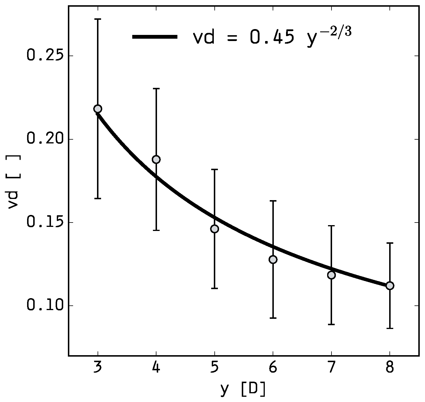
| mean | - | 0.22 | 0.19 | 0.15 | 0.13 | 0.12 | 0.11 |
| SD | - | 0.11 | 0.10 | 0.08 | 0.07 | 0.06 | 0.06 |
© 2016 by the authors; licensee MDPI, Basel, Switzerland. This article is an open access article distributed under the terms and conditions of the Creative Commons Attribution (CC-BY) license (http://creativecommons.org/licenses/by/4.0/).
Share and Cite
Doubrawa, P.; Barthelmie, R.J.; Wang, H.; Pryor, S.C.; Churchfield, M.J. Wind Turbine Wake Characterization from Temporally Disjunct 3-D Measurements. Remote Sens. 2016, 8, 939. https://doi.org/10.3390/rs8110939
Doubrawa P, Barthelmie RJ, Wang H, Pryor SC, Churchfield MJ. Wind Turbine Wake Characterization from Temporally Disjunct 3-D Measurements. Remote Sensing. 2016; 8(11):939. https://doi.org/10.3390/rs8110939
Chicago/Turabian StyleDoubrawa, Paula, Rebecca J. Barthelmie, Hui Wang, S. C. Pryor, and Matthew J. Churchfield. 2016. "Wind Turbine Wake Characterization from Temporally Disjunct 3-D Measurements" Remote Sensing 8, no. 11: 939. https://doi.org/10.3390/rs8110939