Modeling and Reconstruction of Time Series of Passive Microwave Data by Discrete Fourier Transform Guided Filtering and Harmonic Analysis

Abstract

Daily time series of microwave radiometer data obtained in one-orbit direction are full of observation gaps due to satellite configuration and errors from spatial sampling. Such time series carry information about the surface signal including surface emittance and vegetation attenuation, and the atmospheric signal including atmosphere emittance and atmospheric attenuation. To extract the surface signal from this noisy time series, the Time Series Analysis Procedure (TSAP) was developed, based on the properties of the Discrete Fourier Transform (DFT). TSAP includes two stages: (1) identify the spectral features of observation gaps and errors and remove them with a modified boxcar filter; and (2) identify the spectral features of the surface signal and reconstruct it with the Harmonic Analysis of Time Series (HANTS) algorithm. Polarization Difference Brightness Temperature (PDBT) at 37 GHz data were used to illustrate the problems, to explain the implementation of TSAP and to validate this method, due to the PDBT sensitivity to the water content both at the land surface and in the atmosphere. We carried out a case study on a limited heterogeneous crop land and lake area, where the power spectrum of the PDBT time series showed that the harmonic components associated with observation gaps and errors have periods ≤8 days. After applying the modified boxcar filter with a length of 10 days, the RMSD between raw and filtered time series was above 11 K, mainly related to the power reduction in the frequency range associated with observation gaps and errors. Noise reduction is beneficial when applying PDBT observations to monitor wet areas and open water, since the PDBT range between dryland and open water is about 20 K. The spectral features of the atmospheric signal can be revealed by time series analysis of rain-gauge data, since the PDBT at 37 GHz is mainly attenuated by hydrometeors that yield precipitation. Thus, the spectral features of the surface signal were identified in the PDBT time series with the help of the rain-gauge data. HANTS reconstructed the upper envelope of the signal, i.e., correcting for atmospheric influence, while retaining the spectral features of the surface signal. To evaluate the impact of TSAP on retrieval accuracy, the fraction of Water Saturated Surface (WSS) in the region of Poyang Lake was retrieved with 37 GHz observations. The retrievals were evaluated against estimations of the lake area obtained with MODerate-resolution Imaging Spectroradiometer (MODIS) and Advanced Synthetic Aperture Radar (ASAR) data. The Relative RMSE on WSS was 39.5% with unfiltered data and 23% after applying TSAP, i.e., using the estimated surface signal only.

1. Introduction

Microwave radiometers, e.g., the Special Sensor Microwave Imager (SSM/I) and Advanced Microwave Scanning Radiometer for EOS (AMSR-E), are typically on-board sun-synchronous satellites and conically scan the surface with a swath less than 1500 km and a constant incidence angle (see, e.g., [1,2]). The configuration of satellite orbit and scanning leads to observation gaps in a time series of daily microwave observations. Especially when daily observations in only one-orbit direction are used, regularly spaced gaps split the time series into segments. A continuous time series of daily microwave observations in a region is derived by resampling orbit data into a grid system (e.g., [3,4,5]), since the Instantaneous Field Of View (IFOV) of each scan cell does not cover exactly the same region during subsequent scans [6]. Observation errors will be introduced after resampling by the geo-location uncertainty in the center of IFOV (e.g., around 6 km for SSM/I [7]), by the spatial difference between IFOV and grid cell, and by various resampling methods (e.g., [3,4]). These types of errors can have a very large impact when observing coastal regions, lake–land boundaries and mountain areas [8,9,10]. Besides these two kinds of systematic noise, a time series of microwave radiometer observations carries information about surface emittance, vegetation attenuation, atmospheric emittance and atmospheric attenuation. The surface signal includes the former two items and the atmospheric signal includes the latter two. Surface emittance at microwave frequencies is positively related to surface wetness condition [11]. Thus, in order to retrieve surface wetness conditions from microwave observations, influences of vegetation and atmosphere need to be removed. Vegetation influence can be removed by combining data acquired by multiple satellite instruments—microwave radiometers, Synthetic Aperture Radar (SAR), and optical and Infrared (IR) sensors (see, e.g., [12,13,14,15]). In this paper, we developed a hybrid method to extract the surface signal, after removal of the atmosphere influence, observation errors and gaps from a time series of daily microwave observations.

The capability in penetrating clouds and the spatial resolution of a microwave radiometer both depend on the frequency [11], but in an opposite way, i.e., lower frequencies have higher penetrating capability but lower spatial resolution, while higher frequencies have higher spatial resolution but influenced more by atmosphere and vegetation. Thus microwave frequencies not higher than Ka band (26.5–40 GHz) are normally used to monitor surface wetness conditions (e.g., [16,17,18,19,20]). Observation at 37 GHz, is preferred to observe inundated area (e.g., [21,22,23,24,25,26,27,28]), due to its higher spatial resolution than lower frequencies, while retaining sufficient sensitivity to surface wetness. In our previous study [15], the fractional area of Water Saturated Surface, i.e., water saturated soil and inundated area, was retrieved using the Polarization Difference Brightness Temperature (PDBT) observations at 37 GHz, taking the vegetation influence and surface roughness into account. Atmosphere influence on observations at 37 GHz is significant, especially during rainy days [15,29]. Observation errors cause a larger variability in daily PDBT at 37 GHz at lake–land boundaries (e.g., above 40 K Figure 1b) than that of monthly averages on inundated areas (e.g., 20 K in the Pantanal [30]). To eliminate the temperature difference between surface and vegetation canopy, only night or early-morning data at 37 GHz, i.e., in one-orbit direction, are used to retrieve WSS, which leads to a large amount of observation gaps (Figure 1). Thus, noise due to the combination of atmosphere influence, observation gaps and errors must be removed prior to apply 37 GHz PDBT time series to retrieve inundated area.

In other studies [22,23,24,25,26,27], systematic noise was removed by aggregating raw daily data over time and space: gaps can be filled by monthly compositing and observation errors can be mitigated by spatial averaging. The detailed spatial and temporal information about atmospheric and surface water content, however, is also filtered out by temporal compositing and spatial averaging. Atmosphere influence on monthly data can be reduced by two different approaches. The first one is a statistical composition method, i.e., to select the second lowest value in each month as an indicator of the monthly surface wetness condition (e.g., [23,24,25,26]). The second approach is to use ancillary data about atmospheric and land surface properties from other satellites (e.g., cloud fraction and Land Surface Temperature (LST) from International Satellite Cloud Climatology Project (ISCCP), and atmospheric temperature and total precipitable water from TIROS Operational Vertical Sounder (TOVS) products [5,31]) to parameterize the atmosphere influence on emittance at 37 GHz with a radiative transfer model [5] or to apply a neural network inversion method [32]. For daily time series, the first method is not applicable and the second one gives estimates of surface emittance of insufficient accuracy in the presence of clouds or rain (e.g., [5,33,34,35]).

The objective of our study was to develop a hybrid method, named “Time Series Analysis Procedure (TSAP)”, to extract the surface signal from a noisy time series of daily pixel-wise PDBT observations at 37 GHz by filtering out atmosphere signal, observation gaps and errors. TSAP includes two stages: (1) identify the frequency range related to observation errors and gaps and filter them out with a boxcar filter; and (2) identify the atmospheric signal by applying Discrete Fourier Transform (DFT) analysis of precipitation time series and filter them out with the Harmonic Analysis of Time Series (HANTS) algorithm. TSAP is based on the feature extraction from time series with DFT [36,37,38,39,40], commonly used in data mining. EASE-Grid SSM/I 37 GHz brightness temperature data [3] acquired in the early morning pass is used in our case study to illustrate the problems, to explain the proposed method and to validate it. Section 2 introduces the theory of DFT and its properties. Section 3 describes the study area and data set used in our study. Section 4 illustrates the implementation of TSAP in detail and analyzes the mitigation of the noise present in the raw (unfiltered) time series. In Section 5, a case study on Poyang Lake is presented to evaluate TSAP by analyzing the accuracy in the retrieval of the Water Saturated Surface (WSS) area before and after applying TSAP. Finally a large area application is presented on the evolution of the WSS area in dry and wet years over the Poyang Lake and Dongting Lake floodplains. Discussion about TSAP and its performances is articulated in Section 6. Conclusions are summarized in Section 7.

2. The Time Series Analysis Procedure

2.1. General

We regard a time series of daily 37 GHz PDBT as consisting of observation gaps and errors, atmospheric and surface signals. More precisely we consider the atmospheric signal to include atmosphere emittance and attenuation, while the surface signal includes surface emittance and vegetation attenuation. According to the linear and multiplicative properties of DFT, the spectral properties of component signals can be revealed in the power spectrum of the mixed signal, i.e., the PDBT time series. Once the spectral features of each component signal are identified, a proper filter method can be designed to extract the surface signal.

The frequency range associated with observation gaps can be easily identified in the power spectrum of a time series of daily 37 GHz PDBT observations obtained in one-orbit direction. Observation errors are commonly assumed to yield a white noise (see, e.g., [41]), while we noted a high frequency periodic component in the DFT of the PDBT time series. To evaluate these findings, we developed a numerical model (see Section 2.4) to mimic observation gaps and errors. By analyzing the synthetic signal generated with the model and the PDBT time series, we found that the signal components associated with observation gaps and errors are in the higher frequency region. Thus, A boxcar filter is applied to remove the high frequency components (see, e.g., [42]), mainly due to its high coherent gain and narrow equivalent noise bandwidth, compared with other window—based filters [41]. The high scallop loss of a boxcar filter is mitigated by using long-term time series of daily observations. We modified the boxcar filter according to the number of gaps in the PDBT time series (see Section 4.2.1). The transfer function of the modified boxcar filter will be evaluated in Section 4.2.2.

It is often assumed that the changes in atmospheric conditions are much faster than in surface conditions (see, e.g., [5]). This gives an opportunity to separate the atmospheric and surface signals by means of an appropriate filter, provided the associated spectral features can be identified. In our previous study [15] we noted that atmosphere attenuation on PDBT time series at 37 GHz is almost synchronous with precipitation observed on ground, which agree with the findings in [29], where it was noted that the precipitation rate is positively related to the water depth of hydrometeors that contributes to atmosphere emittance and attenuation at 37 GH. This led us to the idea of estimating the frequency range associated with the atmospheric signal by analyzing a time series of rain-gauge data. The risk of this approach is that precipitation also causes changes in soil moisture, which is the major factor controlling the surface signal [21,30]. Studies on field-measured soil moisture, however, show that the soil moisture signal is dominated by seasonal changes (see, e.g., [43,44,45,46,47]), i.e., the characteristic time scale of soil moisture is one to three months. This long-memory of soil moisture is defined as time stability by [45]. On the other hand, ground-measured precipitation time series do show an annual component but no significant seasonal changes [44], with much larger short-term periodic variations than soil moisture [48], i.e., closer to a random process. Thus we can use the power spectrum of precipitation time series to identify the frequency range associated with the large but short-term periodic variations and to design a filter to extract the surface signal in 37 GHz PDBT time series.

We extracted the surface signal by applying HANTS algorithm, first developed by [49] and used to reconstruct cloud-free time series of Normalized Difference Vegetation Index (NDVI) and LST [50,51,52,53]. This algorithm applies user-selected harmonic components to model a signal and algorithm parameters can be set to reconstruct the upper-envelope of a time series of samples. The latter feature removes the atmosphere-affected samples as outliers, since atmospheric influence always attenuates surface PDBT (see Section 4.3).

2.2. Discrete Fourier Transform of a Time Series

An uniformly sampled time series, i.e., f(t_i), with sampling interval Δt and record length P, can be expressed with a Fourier series as:

$$f\left(t_i\right)=\frac{{\mathrm{{\rm A}}}_0}{2}+{\displaystyle \sum _{n=1}^N{\mathrm{{\rm A}}}_n\sin \left(\frac{2\pi n{t}_i}{P}+{\varphi }_n\right)},\mathrm{for}\mathrm{integer},t_i=0,\Delta t,2\Delta t,\dots ,N\Delta t$$

(1)

where A₀ is the average of whole time series, A_n and ${\varphi }_n$ is the amplitude and phase respectively of the harmonic component with cycle number n, N is the largest cycle number involved and also the total sample size, i.e., N = integer of P/ΔT, and t_i is the sampling time. Throughout this manuscript, we use the cycle number n and the corresponding period, instead of frequency. The amplitude and phase of harmonic components in Equation (1) are obtained by calculating the Discrete Fourier Transform (DFT) of f(t_i). According to [54], the DFT of f(t_i) is denoted as x(n) and is defined as:

$$x\left(n\right)={\displaystyle \sum _{t_i=0}^{N\times \Delta t}f\left(t_i\right)\exp \left(\frac{-i2\pi n{t}_i}{P}\right)},\mathrm{for}\mathrm{integer}n\in \left[-\frac{N}{2},\frac{N}{2}\right]$$

(2)

where n is the cycle number involved in Equation (1), t_i is sampling time. The amplitude and phase of each harmonic component in Equation (1) can be calculated as:

$$A_n=\left|x\left(n\right)\right|=\sqrt{\mathrm{Re}{\left(x_n\right)}^2+\mathrm{Im}{\left(x_n\right)}^2},\mathrm{for}\mathrm{integer}n\in \left[-\frac{N}{2},\frac{N}{2}\right]$$

$${\varphi }_n=\arctan \left(\frac{\mathrm{Re}\left(x_n\right)}{\mathrm{Im}\left(x_n\right)}\right),\mathrm{for}\mathrm{integer}n\in \left[-\frac{N}{2},\frac{N}{2}\right]$$

(3)

where Re(x_n) and Im(x_n) is the real and imaginary part of x(n) respectively. The DFT can be calculated using many Fast Fourier Transform (FFT) algorithms. More detailed information about FFT can be found in [54,55,56]. In this case, we used the FFT algorithm in the IDL (Interactive Data Language) software. The power spectrum of a time series is the plot of the squared amplitude against the frequency, cycle number or period.

2.3. The Two Properties of Discrete Fourier Transform

Two important properties of Fourier Transform are needed to analyze the power spectrum of a mixed signal and its component signals, e.g., a time series of daily PDBT space-borne observations:

(1)

Linearity: If f(t_i) is the weighted sum of two component time series, then the DFT of f(t_i), i.e., x(n), is also the weighted sum of the DFTs of two component time series.

(2)

Multiplicative: If f(t_i) is the product of two time series, i.e., g(t_i) and h(t_i), then the DFT of f(t_i), i.e., x(n), is the convolution of the DFTs of two component time series as:

$$x\left(n\right)=x_g\left(n\right)\ast x_h\left(n\right)=\frac{{\mathrm{{\rm A}}}_0^h}{2}\times x_g\left(n\right)+\frac{{\mathrm{{\rm A}}}_0^g}{2}\times x_h\left(n\right)+x_{g\times h}\left(n\right),\mathrm{for}\mathrm{integer}n\in \left[-\frac{N}{2},\frac{N}{2}\right]$$

(4)

where * is the convolution operator; $\frac{{\mathrm{A}}_0^g}{2}$ and $\frac{{\mathrm{A}}_0^h}{2}$ is the average of g(t_i) and h(t_i), respectively; and x_g×h(n) is the side lobes introduced by the convolution operator. This property was analyzed by [57].

The two properties can be easily proven by expressing both component time series with Fourier series. These properties are very useful to understand the contribution of each component signal in the DFT of PDBT time series, since both the radiative transfer model in Equation (5), used to describe surface and atmospheric signals, and the numerical model in Equation (7), used to describe the observation errors and gaps, only include the linear and product operators.

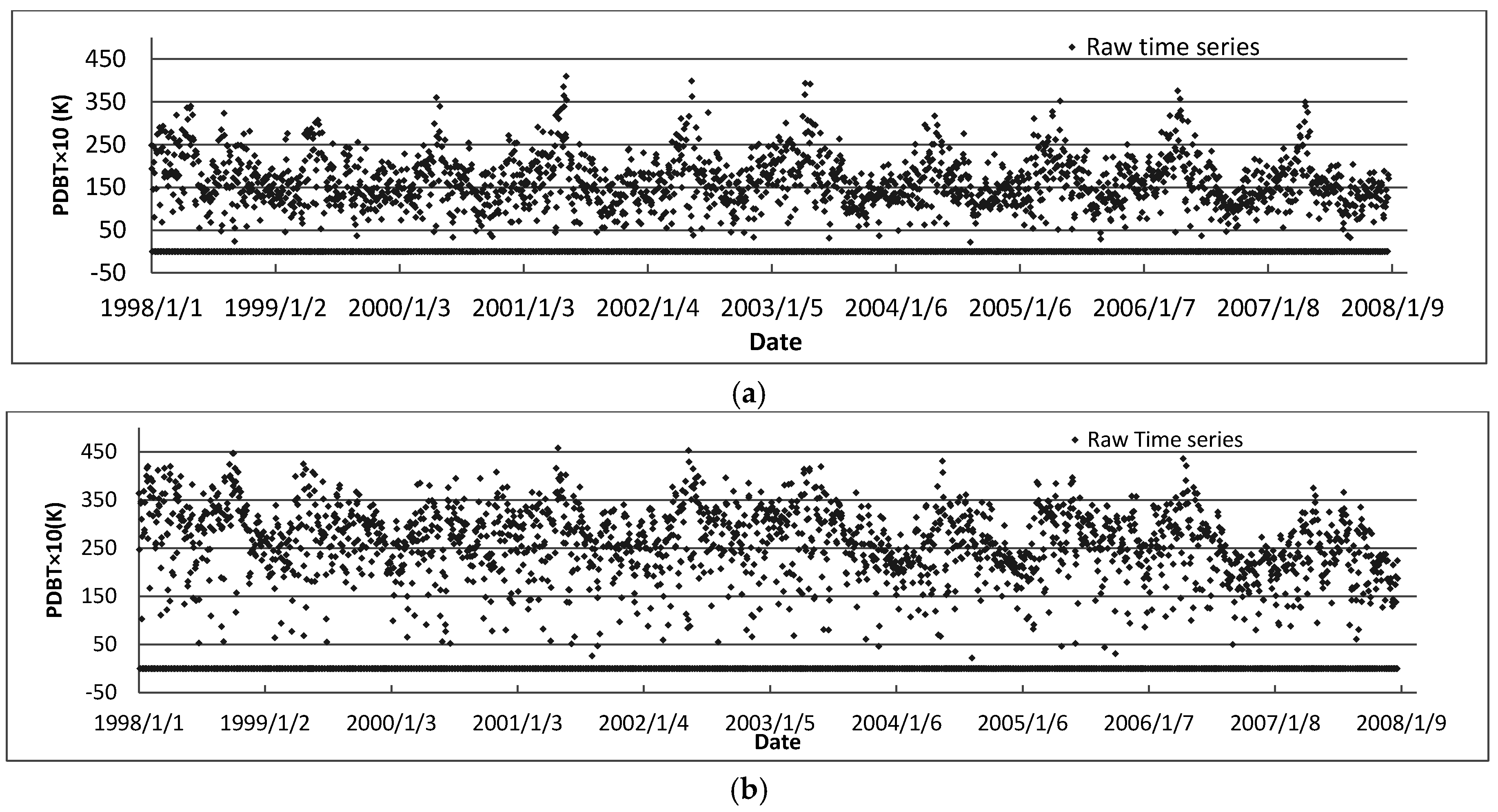
2.4. Numerical Model of a Time Series of Daily PDBT Space-Borne Observations

This section describes a simple model used to simulate how observation gaps and errors, atmospheric and surface signals concur to yield a time series of 37 GHz PDBT observations. We use this model to explain how we can identify each component in actual time series and how we design the filters applied in Stages 1 and 2 of TSAP to extract the surface signal.

A space-borne radiometer measures surface and atmospheric emittance, which are attenuated by atmosphere [29]. Thus a time series of gap-and-noise-free daily PDBT observations at bare soil includes the surface and atmospheric signals, of which the former is the polarization difference of surface emittance and the later includes the down-welling atmospheric emittance reflected and polarized by the surface and atmosphere attenuation [21]. According to the Rayleigh-Jeans approximation, emittance measured by microwave radiometry can be linearly related to the brightness temperature. Thus the PDBT time series at 37 GHz, i.e., ΔT(t_i), can be described by the following radiative transfer model [1]:

$$\begin{gathered} \Delta T\left(t_i\right)=\left[R_h\left(t_i\right)-R_v\left(t_i\right)\right]\times T_s\left(t_i\right)\times t_a\left(t_i\right)+\left[R_v\left(t_i\right)-R_h\left(t_i\right)\right]\times T_d\left(t_i\right)\times t_a\left(t_i\right) \\ {t}_i=0,\Delta t,2\Delta t,\dots ,N\Delta t \end{gathered}$$

(5)

where R_h(t_i) and R_v(t_i) is the effective reflectivity of the surface for horizontal and vertical polarization, T_s(t_i) is the surface temperature, T_d(t_i) is the down-welling apparent brightness temperature of the atmosphere, and t_a(t_i) is the atmospheric transmission function, at t_i. Surface wetness determines the polarization difference in surface reflectivity. Thus the surface signal carries information on surface temperature and soil wetness, while the atmospheric signal carries information on down-welling atmospheric emittance and atmospheric attenuation. In our method to retrieve WSS [15] we take attenuation by vegetation into account, while here is neglected since we only intend to illustrate how the signal components can be identified by time series analysis and filtered to extract the surface signal.

Taking into account the two properties of DFT (Section 2.2), the DFT of the time series of gap-and-noise-free daily PDBT, i.e., x_ΔT(n), can be expressed as:

$$x_{\Delta T}\left(n\right)=a_1\times x_s\left(n\right)+a_2\times x_a\left(n\right)+x_{s\times a}\left(n\right),\mathrm{for}\mathrm{integer}n\in \left[-\frac{N}{2},\frac{N}{2}\right]$$

(6)

where x_s(n) and x_a(n) is the DFT of the surface and atmospheric signals, respectively, x_s×a(n) is the DFT of side lobes introduced by the product of surface and atmospheric signals (see Equation (5)), and a₁ and a₂ is the average of atmosphere signal and surface signal, respectively.

The radiometers on board sun-synchronous satellites introduce observation gaps and errors in the time series of daily PDBT space-borne observations. All gaps are set as 0 and occur periodically in the time series. Thus, we can express this term in the time series of daily PDBT space-borne observations, i.e., f₁(t_i), by adding a noise function to ΔT(t_i) and multiplying it with a square wave as:

$$\begin{gathered} f_1\left(t_i\right)=S\left(t_i\right)\times \left[\Delta T\left(t_i\right)+\alpha \left(t_i\right)\right], S\left(t_i\right)=\{\begin{array}{c}1L_1<t_i\le L\\ 00\le t_i\le L_1\end{array} \\ \mathrm{and}S\left(t_i+L\right)=S\left(t_i\right),t_i=0,\Delta t,2\Delta t,\dots ,N\Delta t \end{gathered}$$

(7)

where S(t_i) is the square wave, α(t_i) is the noise function, all gaps are set to 0, L₁ is the duration of one gap segment and L is the period of the square wave. Since S(t_i) is a piece-wise continuous function, according to the two properties of DFT, the DFT of f₁(t_i), i.e., x_f1(n), can be calculated as:

$$x_{f1}\left(n\right)=a_3\times x_{\Delta T}\left(n\right)+a_3\times x_{\alpha }\left(n\right)+a_4\times x_w(n)+x_{\Delta T\times w}\left(n\right)+x_{\alpha \times w}\left(n\right),\mathrm{for}\mathrm{integer}n\in \left[-\frac{N}{2},\frac{N}{2}\right]$$

(8)

where x_α(n) and x_w(n) is the DFT of observation error and the square wave, respectively, x_ΔT×w(n) and x_α×w(n) is the side lobes introduced by multiplying the square wave with ΔT(t_i) and α(t_i), respectively, a₃ is the average of the square wave and a₄ is the average of the summation of ΔT(t_i) and α(t_i).

Inserting the DFT of ΔT(t_i) (Equation (6)) into Equation (8), the DFT of f₁(t_i) can be calculated from its component signals as:

$$\begin{gathered} x_{f1}\left(n\right)=a_3\times a_1\times x_s\left(n\right)+a_3\times a_2\times x_a\left(n\right)+a_3\times x_{\alpha }\left(n\right)+a_4\times x_w(n)+a_3\times x_{s\times a}\left(n\right)+x_{\Delta T\times w}\left(n\right)+x_{\alpha \times w}\left(n\right), \\ \mathrm{for}\mathrm{integer}n\in \left[-\frac{N}{2},\frac{N}{2}\right] \end{gathered}$$

(9)

Equation (9) shows that the spectral features of component signals also will appear in the power spectrum of the time series of daily PDBT space-borne time series, i.e., f₁(t_i), although the power values will be different from the power spectrum of component signals alone, because the harmonic components in f₁(t_i) also contain contributions from other component signals as shown in Equation (9). This important property helps us to identify which spectral features are due to which component signals.

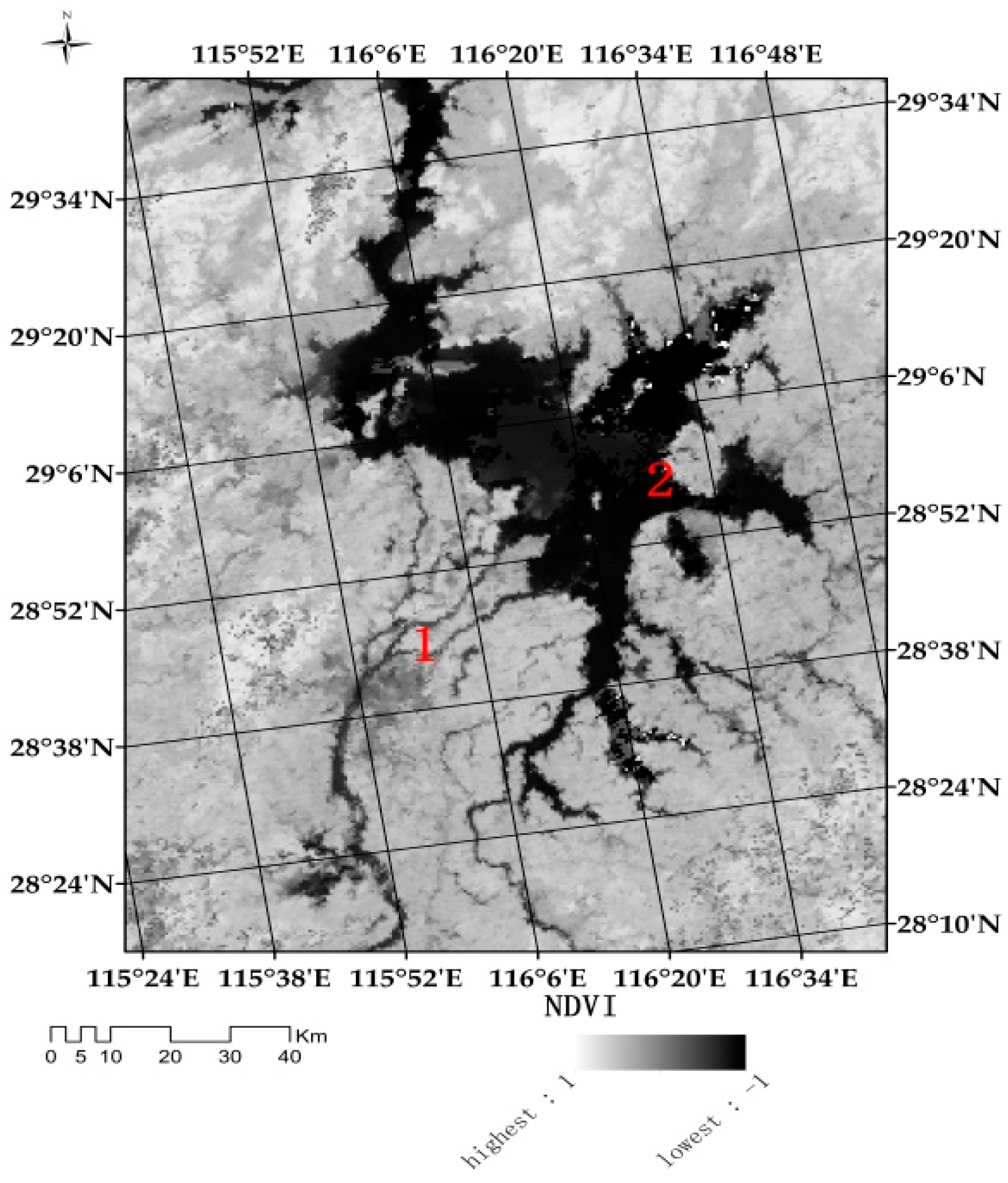
3. The Study Area and Data Set

To demonstrate and validate the TSAP, a case study on the Poyang Lake floodplain, located between 27.50°N and 29.38°N, and from 115.10°E to 117.25°E, was carried out. The two sample pixels in Figure 1 are within the Poyang Lake floodplain (Figure 2). Poyang Lake is the largest lake in the Yangtze River Basin, located between 28.05°N and 29.38°N, and from 115.44°E to 117.00°E. There is a clear dry season from October to March and the flooding season is from April to September. Ten EASE-Grid pixels are needed to cover the whole Poyang lake area, including the 2nd sample pixel in Figure 1. The SSM/I early morning data was used in [15] to retrieve the WSS area of Poyang Lake, with the auxiliary data of MOD09A1 to model the vegetation influence on microwave observation. The retrieval method of WSS is a two-step model: 1st step to retrieve Polarization Difference Effective Emissivity (PDEE) from PDBT and 2nd step to retrieve fractional WSS area from PDEE with a linear model [15]. Considering the large footprint of SSM/I (25 km × 25 km), the spatial heterogeneity is very large at the lake–land boundary area, i.e., a mixture of dry land surface, wet land and lake area. The length of the observation period is ten years, from 1998 to 2007. The rain-gauge data at the two sample pixels was used to estimate the spectral features associated with the atmospheric signal. The Lake areas observed by [58] from MODerate-resolution Imaging Spectroradiometer (MODIS) and Advanced Synthetic Aperture Radar (ASAR) were used to validate the application of the TSAP described in this study to the PDBT time series.

4. Implementation of the Time Series Analysis Procedure

The application of Time series Analysis Procedure (TSAP) includes the following steps:

1

Identify the frequency range of observation gaps and errors.

2

Remove the observation gaps and errors with a boxcar filter.

3

Identify the harmonic components associated with the surface signal.

4

Extract the surface signal from the filtered PDBT time series with the HANTS algorithm.

In this section, the two sample pixels (their PDBT time series shown in Figure 1) are used to demonstrate and analyze each step of the method. Observation gaps and errors in PDBT time series can be identified by comparing the power spectrum of PDBT and of square waves (Section 4.1). They can be removed by a boxcar filter, designed as described in Section 4.2. The atmospheric signal is difficult to identify directly, thus the power spectrum of a precipitation time series is used estimate the characteristic frequency range (spectral features) of atmospheric signal (Section 4.3). The atmospheric signal is removed by reconstructing the surface signal in the PDBT time series by applying the HANTS algorithm (Section 4.4). Statistics are analyzed to evaluate the performance of the boxcar filter and of the HANTS algorithm.

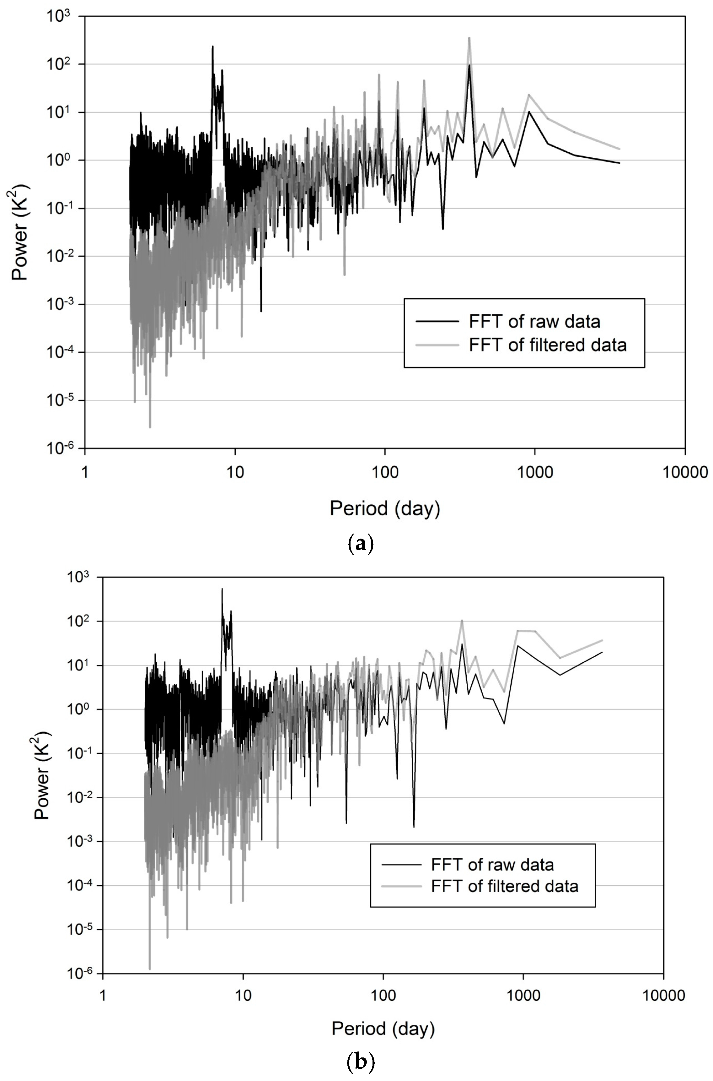
4.1. The Frequency Range of Observation Gaps and Errors

Almost 50% of samples in the time series of daily PDBT observations are gaps, i.e., $L_1=\frac{L}{2}$ in Equation (7). Thus, a square wave S₁(t) with phase = 0 and an unit amplitude can be expressed with a Fourier series [59] as:

$$S_1\left(t_i\right)=\frac{1}{2}+\frac{2}{\pi }{\displaystyle \sum _{m=1,3,5,\cdots }^{\infty }\frac{1}{m}}\sin \left(\frac{2\pi t_i}{P}\times \frac{mP}{L}\right),t_i=0,\Delta t,2\Delta t,\dots ,N\Delta t$$

(10)

where mP/L is the cycle numbers of harmonic components applied to represent S₁(t_i). The length of the observation period, i.e., P, is 10 years for the two sample pixels in Figure 1, while L, the period of a square wave in a PDBT time series, is normally of the order of a few days, thus mP/L is very large, i.e., the harmonic components of S₁(t_i) lie in the high frequency range. In the power spectrum of these two examples (Figure 3), there are two extreme high peaks in the high frequency range (i.e., short periods): one with a period of seven days, and the other with a period of eight days. When L = 8 days, the power spectrum of Equation (10) is shown in Figure 4a. The largest peak of this square wave equals to eight days and the second largest peak equals to 8/3 days (Figure 4a). This means that the other extreme high peak in the power spectrum of f₁(t_i) (Figure 3) does not come from the square wave with L = 8 days, but comes from another square wave, i.e., S₂(t_i) with L = 7 days as Figure 4b shows.

These two square waves split the whole time series into three stages (Figure 1): (1) gaps with value of 0; (2) observations with values averaging around 5 K in Figure 1a and 10 K in Figure 1b; and (3) observations with values around 15 K in Figure 1a and 25 K in Figure 1b. When the rain rate is around 25 mm/h, the modeled up-welling PDBT at 37 GHz has been shown to be around 5 K for various land cover types [60]. This strong attenuation by heavy precipitation leads to many observations with values around 5 K in Figure 1a and values around 10 K in Figure 1b. These attenuated observations periodically occur in the time series of PDBT observations according to its DFT in Figure 3, but we did not find such evidence in the DFT of time series of ground-measured precipitation. This implies that the periodic influence of precipitation on PDBT observations is probably due to a periodic component in the observation errors, e.g., the periodic scan configuration in SSM/I [6] may lead to these periodic sampling errors. Thus, we can assume that the observation errors consist of one non-periodic component, i.e., white noise, and one periodic component, i.e., the square wave with L = 7 days or L = 8 days.

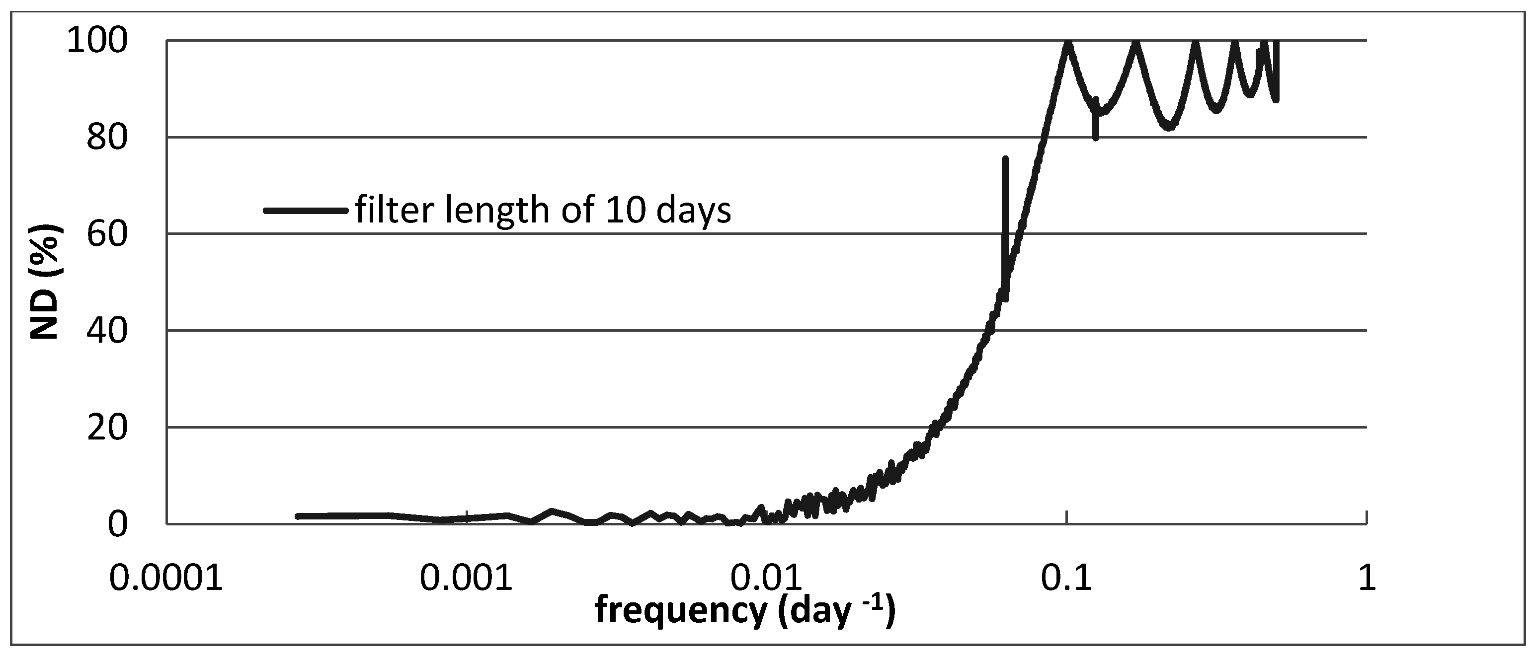
4.2. The Modified Boxcar Filter and Its Transfer Function

4.2.1. The Modified Boxcar Filter

The power spectrum of the PDBT time series of both sample pixel 1 and 2 (Figure 3) shows two clear peaks with periods of seven and eight days. Using Equation (8), we generated a time series with two square-wave components with periods of seven and eight days: the power spectrum of this time series (Figure 4) shows that the two peaks at seven and eight days in Figure 3 can indeed be explained by two square-wave components, i.e., one due to gaps and the other due to observation errors. To filter out the harmonic components due to observation gaps and errors in the raw PDBT time series, we applied a modified boxcar filter, by adapting the filter length to the gap size and location:

$$f_2\left(t_i\right)=\frac{{\displaystyle \sum _{k=t_i-M}^{t_i+M}{f}_1\left(k\right)}-\min {[f_1\left(t_i-M\right),\cdots ,f_1\left(t_i+M\right)]}_{unzero}-\max {[f_1\left(t_i-M\right),\cdots ,f_1\left(t_i+M\right)]}_{unzero}}{S_M-2}$$

(11)

where $f_1\left(k\right)\in \left[f_1\left(t_i-M\right),f_1\left(t_i-M+1\right),\cdots ,f_1\left(t_i+M-1\right),f_1\left(t_i+M\right)\right]$, which is a subset symmetric with center at t_i, 2 × M is the filter length, [f₁(t_i − M), f₁(t_i − M + 1),…, f₁(t_i + M − 1), f₁(t_i + M)]_unzero means non-zero elements. In each subset, S_M is the number of non-zero elements. S_M varies through the time series, i.e., $t_i\in \left[0,1,\cdots ,N\right]$. The minimum non-zero value in each subset is filtered out in Equation (11), to reduce the impacts of the strong attenuation due to heavy rainfall or clouds. The maximum value is also filtered out, as suggested by [5].

The minimum length of a boxcar filter depends on the lowest frequency of square-wave components in PDBT (see, e.g., [61]). There must be at least 1 non-zero observation available, i.e., S_M > 2 in Equation (11), within the interval 2 × M. The maximum length of gaps, i.e., numbers of samples with value of 0 in the interval 2 × M, occurs at the beginning and end of the time series. To guarantee S_M >2, the minimum filter length can be calculated as:

$${\left[2\times M\right]}_{\min }=L+2$$

(12)

where L is the period of the square wave. With this minimum length of 10 days, the modified boxcar filter in Equation (11) can filter out all frequencies higher than the lowest frequency associated with observation gaps and errors, i.e., with shorter periods than the maximum period of the two square waves, i.e., L = 8 days in Figure 3.

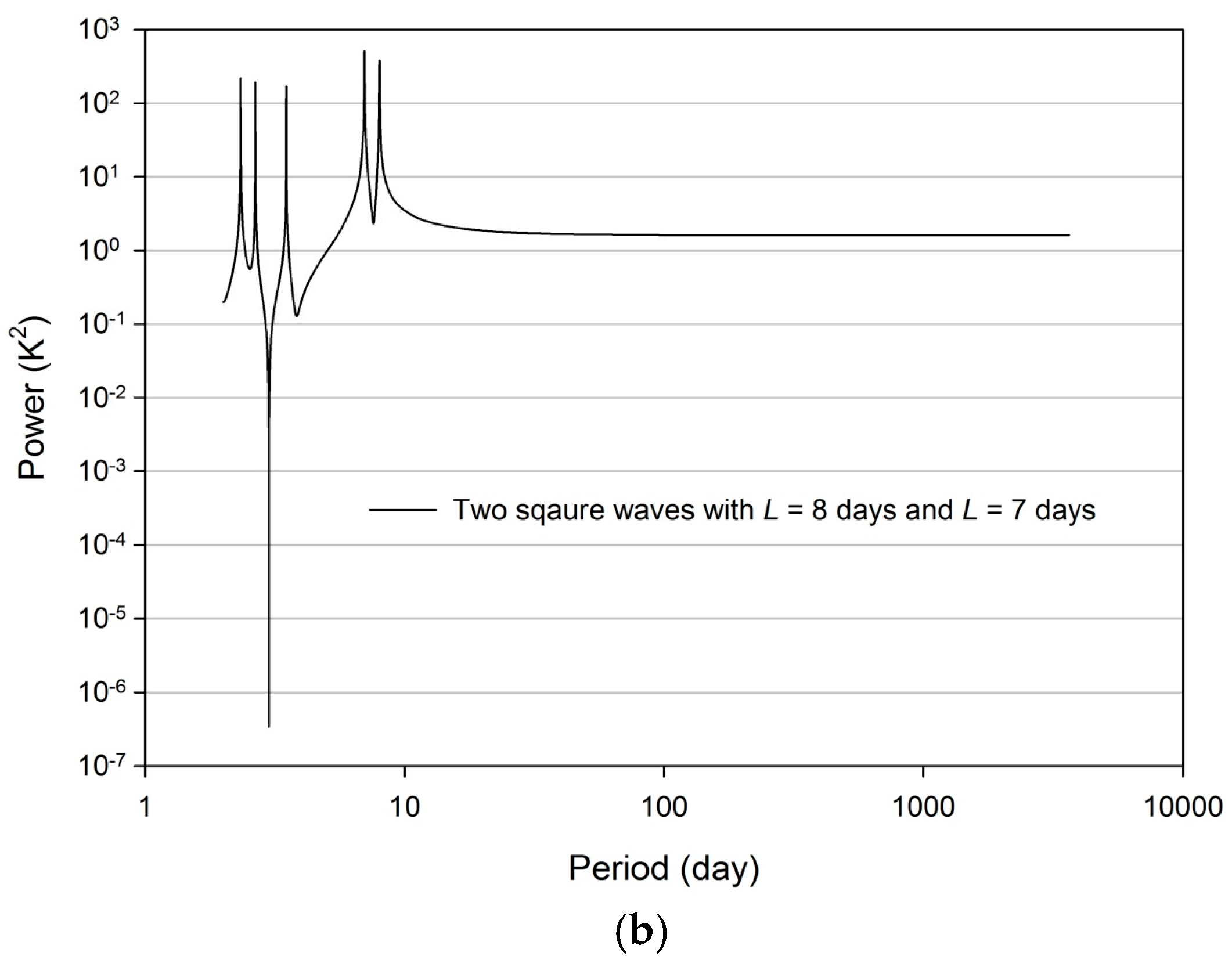
4.2.2. On the Transfer Function of the Modified Boxcar Filter

The modified boxcar filter is a low pass filter, thus it can filter out the frequencies with periods shorter than the maximum period of the observation gaps and errors components and retain the frequencies with longer periods. The question is whether the modified boxcar filter modifies the lower frequency components. If we represent the noise-and-gap-free PDBT time series with harmonic components (Equation (1)), we can evaluate the transfer function of the boxcar filter in the frequency domain. We assumed that the power due to observation errors is half of the total power in the PDBT time series according to the Parseval’s theorem. In this way, we can calculate the processing loss of the modified boxcar filter as follows.

g_n(t_i) is a harmonic component in the noise-and-gap-free PDBT time series with cycle number n:

$$g_n\left(t_i\right)={\mathrm{{\rm A}}}_n\sin \left(\frac{2\pi n{t}_i}{P}\right),t_i=0,\Delta t,2\Delta t,\dots ,N\Delta t$$

(13)

where A_n is the amplitude of the harmonic component in f(t_i) and P is the length of observation period. In our experiment, P = 10 × 365 days. Adding the white noise to g_n(t_i) and multiplying it with S₁(t_i) (Equation (10)), we can get a gappy-and-noisy time series:

$$g_n^1\left(t_i\right)={\mathrm{{\rm A}}}_n\left[\sin \left(\frac{2\pi n{t}_i}{P}\right)+{\alpha }_0\left(t_i\right)\right]\times S_1\left(t_i\right),t_i=0,\Delta t,2\Delta t,\dots ,N\Delta t$$

(14)

where α₀(t_i) is the white noise due to the observation errors with the same amplitude as the amplitude of this component. The noise floor level in the PDBT time series is around 0.2 K due to calibration errors according to [10], much less than the possible variation due to observation errors, thus it is negligible in this study. After applying the modified boxcar filter in Equation (11), we get the filtered time series as:

$$g_n^2\left(t_i\right)={\mathrm{{\rm A}}}_n^F\sin \left(\frac{2\pi n{t}_i}{P}\right),t_i=0,\Delta t,2\Delta t,\dots ,N\Delta t$$

(15)

where ${\mathrm{A}}_n^F$ is the amplitude after filtering. The normalized difference between the gap-and-noise-free amplitude and filtered amplitude for each harmonic component, i.e., ND_n, is used to represent the processing loss of the filter and is defined as:

$$N{D}_n=\left|\frac{{\mathrm{{\rm A}}}_n^F}{{\mathrm{{\rm A}}}_n}-1\right|\times 100\%$$

(16)

ND_n does not depend on A_n. To simplify our analysis, we set A_n = 1.0 for all tested n belonging to [1, 2, 3,…, N]. Smaller ND values mean less processing loss after applying the modified boxcar filter.

According to the power spectrum of PDBT observations in Figure 3, the maximum period of the two square waves is eight days, thus the minimum filter length (according to Equation (12)) is 10 days and the period of the square wave introduced in this experiment is eight days. The white noise is generated using the RONDOMU function in IDL. Since the FFT algorithm calculates frequencies with cycle number in the range of [−N/2, N/2], we only analyze n ϵ [1, 2, 3,…, N/2], with N = 3650. When frequency ≥0.05, i.e., periods ≥20 days, the ND values are all above 40% (Figure 5), which indicates that the components with higher frequency have been filtered out by the modified boxcar filter.

4.3. Identify the Spectral Features of the Surface Signal

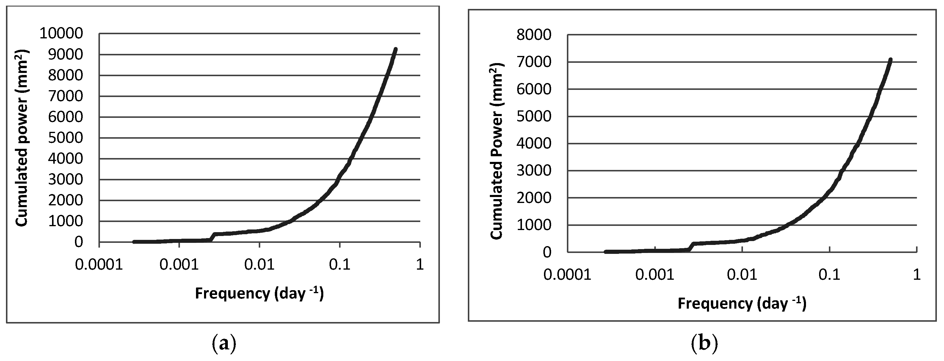
4.3.1. Identify Frequency Range of Atmospheric Signals from Precipitation Time Series

The atmospheric attenuation and the down-welling atmospheric emittance are both primarily controlled by precipitable water hydrometeors [21,29]. Satellite retrievals of both daily total precipitable water content and precipitation have large uncertainties over land (see, e.g., [33,34]), hence it is difficult to identify spectral features related to atmospheric signal by analyzing satellite data. The occurrence of precipitation correlates with large clouds [62] and we observed (see Figure 6) large drops in the filtered PDBT time series during precipitation events. Accordingly, we used the time series of rain-gauge data to identify the spectral features associated with the atmospheric signal.

The cumulated power spectrum of the rain-gauge time series at two locations (Figure 7) shows that most of the variability is associated with harmonic components at frequencies >0.00274 day⁻¹, i.e., periods <73 days. Moreover, there is a jump in the cumulated power spectrum at a frequency of 0.0137 day⁻¹, i.e., period = 365 days. Since components with periods <20 days have been filtered out by applying the boxcar filter (see Figure 5), we may conclude that the spectral features associated with the atmospheric signal have periods range of [20 days, 73 days].

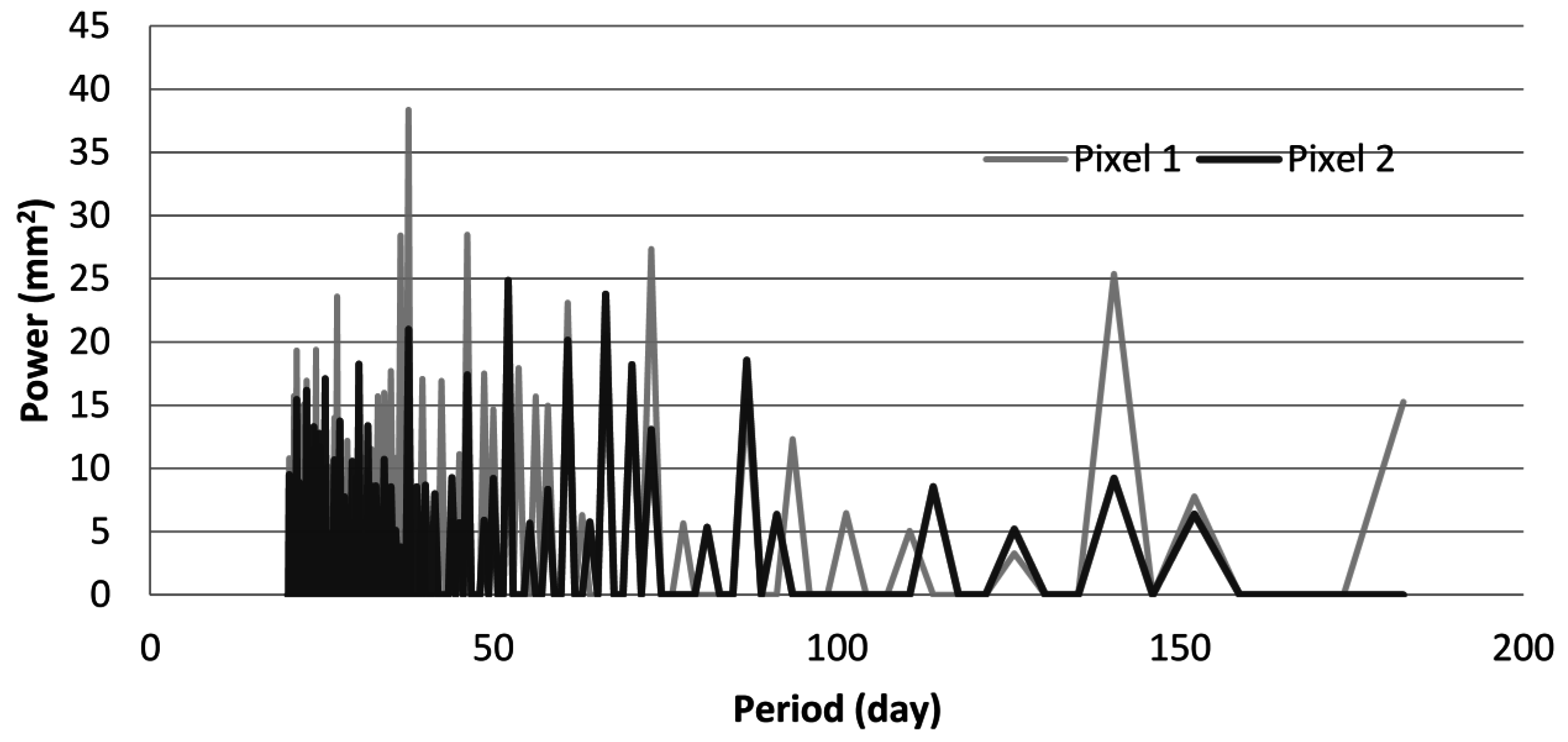
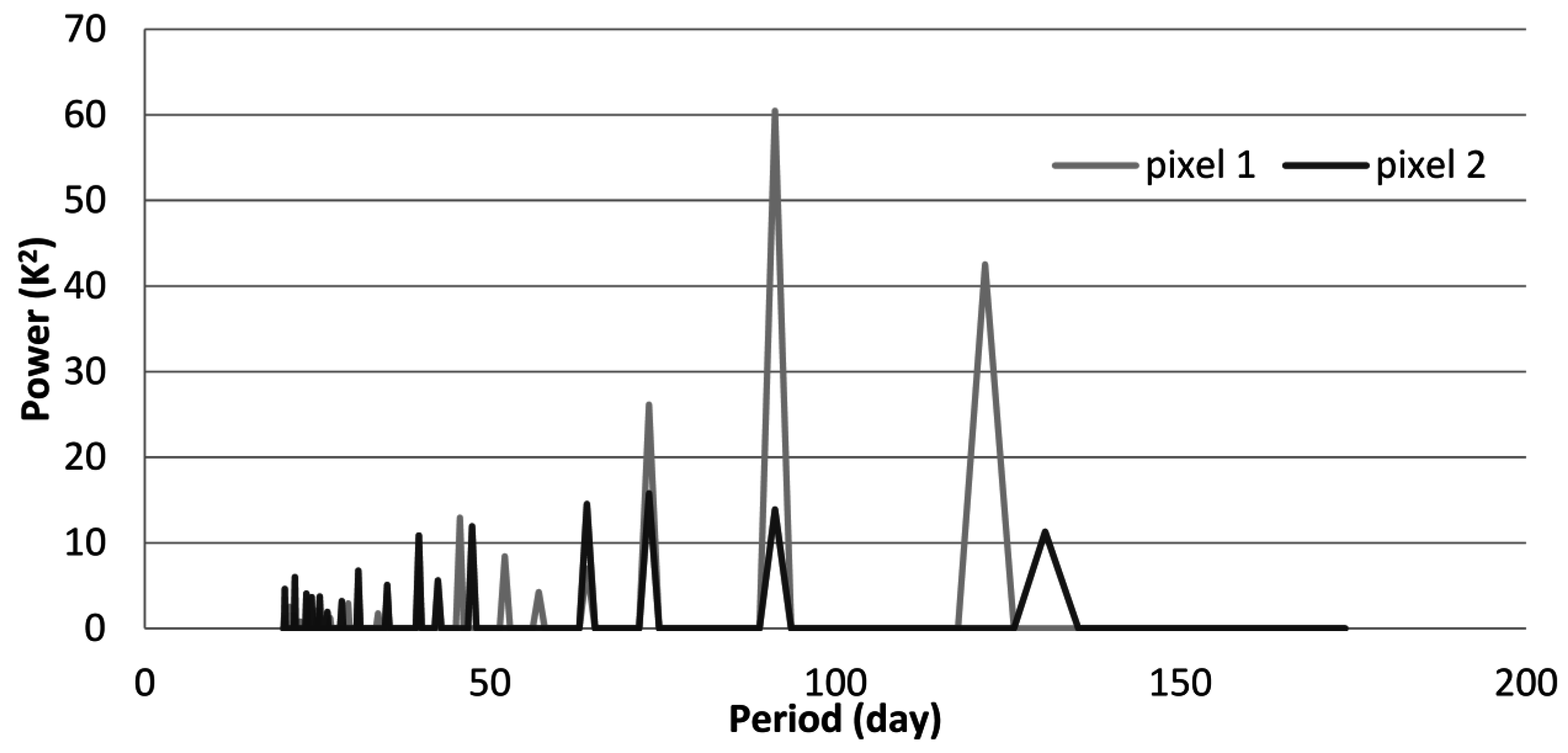
4.3.2. Identify the Spectral Features of the Surface Signal

To identify more precisely the surface signal, we have compared the power spectrum of the rain-gauge time series at higher frequencies (Figure 8) with the power spectrum of the boxcar-filtered PDBT time series (Figure 9). Most of the variability in rain-gauge time series is accounted for by high frequency component, more precisely the ones having periods between say 20 and 73 days (Figure 8). On the other hand most of the variability in the PDBT time series is accounted for by components at lower frequencies, namely the components with periods >73 days (Figure 9). This confirms the conclusion that atmospheric signal in the PDBT time series is accounted for by components with periods in the range [20 days, 73 days], while the surface signal is associated with components having periods >73 days.

In the main lobe peaks of the PDBT time series (Figure 9), we also noticed several components that are not associated with the atmospheric signals in the range 20–73 days (

Table 1. Surface components, i.e. harmonic components associated with the surface signal, with shorter period (higher frequency) than the threshold component = 73 days in the 10-year time series.

Pixel Location	Period of Surface Components (Days)
The 1st sample	64, 57, 46, 34, 31, 25, 23, 20
The 2nd sample	47, 42, 40, 31, 29, 26, 25, 23

). These components may represent the short-term variations in the surface signal.

4.4. Extract the Surface Signal from the Filtered PDBT Time Series by HANTS

Having identified the spectral range associated with the surface signal, we can represent the PDBT time series as:

$$f_s^1\left(t_i\right)=A_0^s+{\displaystyle \sum _{j\in R^s}{A}_j^s\times \sin \left(\frac{2\pi j}{N}{t}_i+{\varphi }_j^s\right)},t_i=0,\Delta t,2\Delta t,\dots ,N\Delta t$$

(17)

where $f_s^1\left(t_i\right)$. is the surface signal and (j/N) gives periods ≥20 days, i.e., it is expressed by the harmonic components due to the surface signal—$j\in R^s$; $R^s$ is the spectral features of the surface signal. It is reasonable to assume that the upper envelope of the filtered PDBT time series (Figure 6) consists only of the samples without or with less atmospheric attenuations. The HANTS algorithm estimates the amplitudes and phases in Equation (17) through an iterative procedure that ends when the following constraint is met:

$$\min \left|f_s^1\left(k_i\right)-f_1\left(k_i\right)\right|\le e$$

(18)

where k_i is sampling time, $f_s^1\left(k_i\right)$ is the modeled value using HANTS algorithm with Equation (17), and e is the user-prescribed errors of reconstruction (see [52] for a detailed explanation of HANTS parameter setting). If values much lower than the reconstructed time series are regarded at outliers, HANTS gives a reconstruction close to the upper envelope as the example shown in Figure 6.

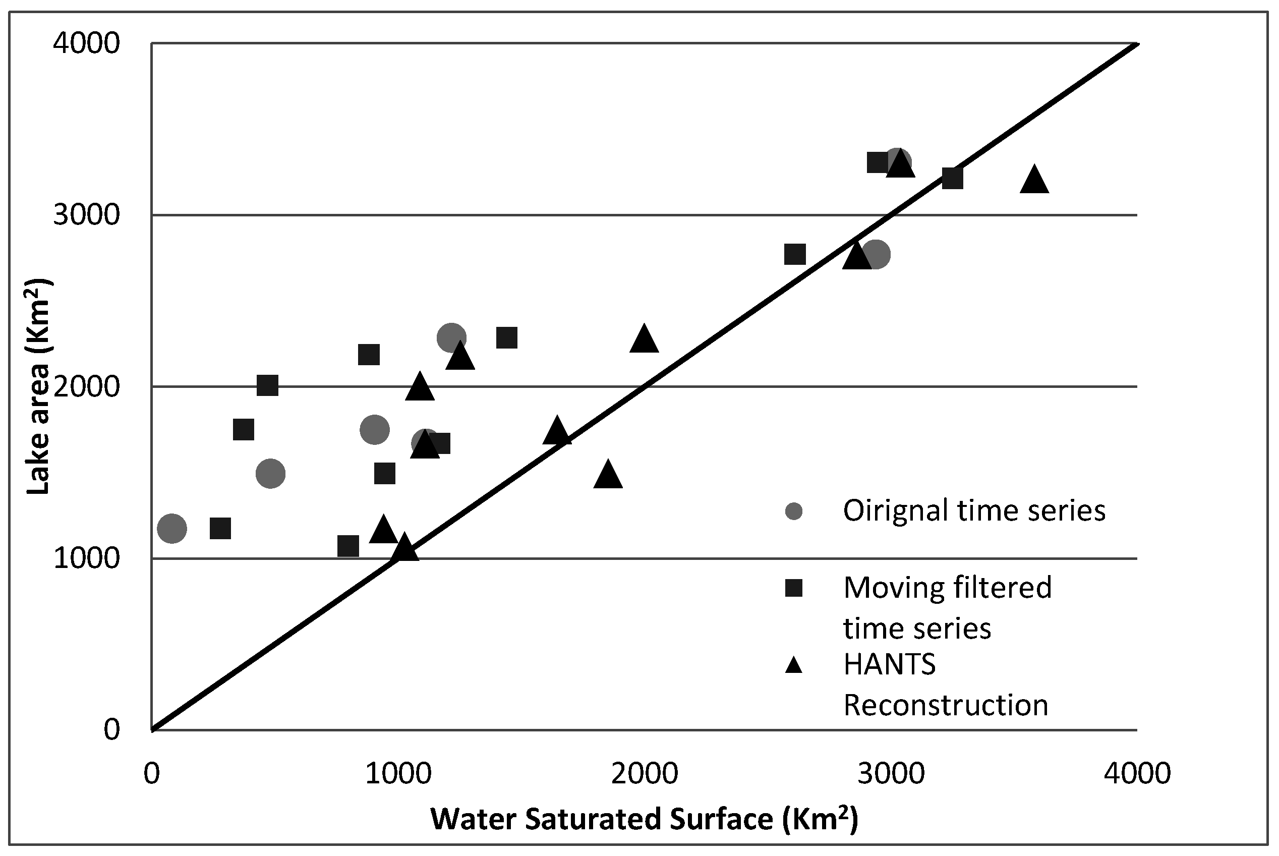
4.5. Statistical Evaluation of TSAP

A statistical summary (

Table 2. Statistical summary on original, boxcar filtered, and reconstructed PDBT time series.

	1st Example at Crop Land			2nd Example at Lake Area
	Raw Data	Boxcar Filter	HANTS	Raw Data	Boxcar Filter	HANTS
non-zero Minimum (K)	2.2	7.4	10.6	2.2	12.6	18.7
Maximum (K)	41	34.3	35.1	45.8	40.8	42.5
Mean (K)	16.1	16.2	18.9	25.9	26.4	29.8
Std (K)	9.2	4.3	4.5	14	4.6	4.3

) about raw, boxcar filtered and HANTS reconstructed PDBT time series shows that the averaged and non-zero minimum values of time series both increased after each step of TSAP. This indicates that after each step of TSAP, lower values, which are due to observation errors or due to atmosphere attenuation, have been replaced by higher values in the time series. The maximum value is assumed to be a correct observation in the raw data. The maximum values after HANTS reconstruction were closer to the raw data than those after boxcar filtering, in both samples. It means that HANTS improved the representation of the time series, compared with the boxcar filtering. After the reconstruction, the range over open water area was reduced from 43.6 K (raw data) to 24.8 K that is close to the expected range of PDBT over inundated areas observed by [30]. The Root Mean Square Deviation (RMSD) was calculated between two time series after each step of TSAP (

Table 3. Root Mean Square Deviation (RMSD) at each step in TSAP.

	1st Example at Crop Land		2nd Example at Lake Area
	Raw—Boxcar Filter	Boxcar Filter—HANTS	Raw—Boxcar Filter	Boxcar Filter—HANTS
RMSD (K)	11.7	4.4	18.1	5.5

). The large decrease in standard deviations (Table 2) from the raw data to the boxcar-filtered time series came together with large RMSD between them, mainly related to the power reduction in the frequency range associated with observation gaps and errors after filtering in Figure 3. This means most of the noise in the raw data was removed by the modified boxcar filtering. The standard deviations of boxcar filtered and HANTS reconstructed time series were similar, but the RMSD between them was not negligible, although smaller than the RMSD between the raw and filtered time series. The improvements in HANTS reconstructed time series were mainly the representation of the upper envelope and the mitigation of the impact of atmospheric attenuation, as shown by higher values of mean, minimum, and maximum compared with the boxcar filtered time series (Table 2).

5. Case Study in the Poyang Lake and Dongting Lake Floodplains

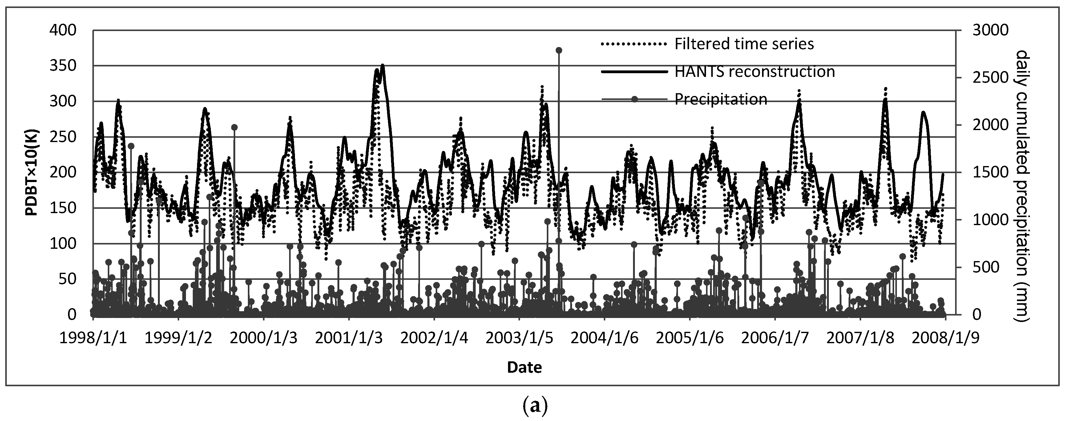
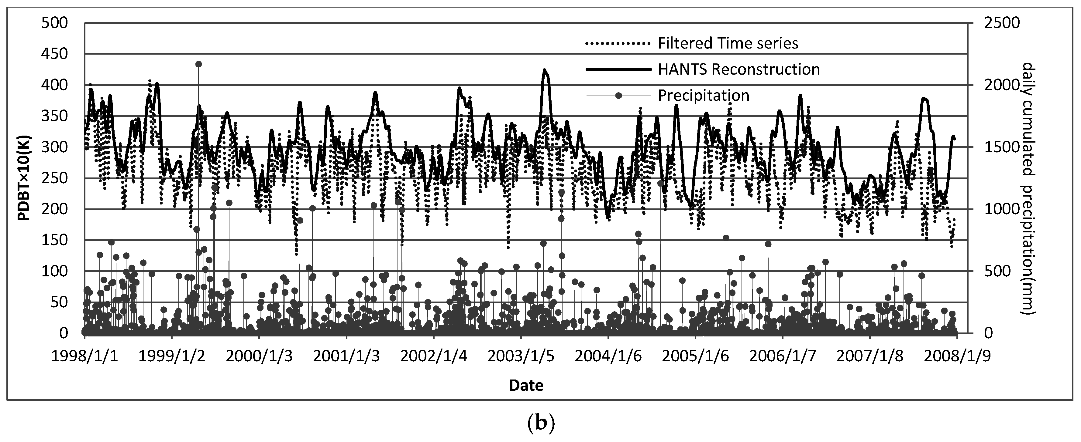
5.1. Time Series Analysis Procedure Applied to the Poyang Lake Area

In the first stage of TSAP, the DFT of 37 GHz PDBT time series is used to identify the spectral range associated with gaps, i.e., L = 8 days in our case. This value is rather uniform in the Poyang Lake area, which gives a minimal filter length of 10 days, according to Equation (12). In the second stage of TSAP, the DFT of the time series of rain-gauge data is used to identify the frequency range associated with the atmospheric signal. The threshold frequency separating the surface and atmospheric signals can be estimated by analyzing the difference between the power spectrum of precipitation time series and the filtered PDBT time series. It is found that this threshold value is almost constant in Poyang Lake and it gives a period equal to 73 days. All the harmonic components at frequencies lower than this threshold are due to the surface signal. The harmonic components listed in the 2nd sample pixel of Table 1 are also due to the surface signal, but with periods <73 days. These harmonic components are used to extract the surface signal with HANTS for each pixel.

5.2. Case Study: Poyang Lake

To evaluate the performance of TSAP, we applied it to the ten pixels covering Poyang Lake to retrieve its WSS area, i.e., open water area and water saturated soil surface (see [15]), using the PDBT observations at each stage of TSAP. The WSS is calculated from the Polarization Difference Effective Emissivity (PDEE) with a linear model, where the surface roughness is considered. More detailed information about the retrieval of WSS can be found in [15].

The retrieved WSS at each stage has been evaluated against lake area observed at higher spatial resolution data with MODerate-resolution Imaging Spectroradiometer (MODIS) and Advanced Synthetic Aperture Radar (ASAR). Thus we compared the WSS retrieved with three PDBT data sets, i.e., original PDBT observations, boxcar-filtered PDBT data and HANTS-reconstructed PDBT data, with the lake area estimated with MODIS and ASAR images by [58] (Figure 10). Though the R² is higher when using the original PDBT, its relative RMSE is also larger (

Table 4. Correlation of retrieved Poyang lake area with PDBT in different stages of TSAP and observations by [58], and their relative RMSE.

	R2	RMSE (km2)	Relative RMSE
Original Time series	0.9195	802.14	38.48%
boxcar filtered	0.7845	866.93	41.59%
HANTS Reconstruction	0.7747	479.33	22.99%

) and the retrieved WSS area is much less than the observed lake area, while WSS area is the sum of lake area, wet land and water saturated soil, i.e., it should be WSS >lake area. The retrieved WSS areas with the HANTS reconstructed surface signal has the lowest R² value but the best relative Root Mean Square Error (RMSE), and samples are located around the 1:1 line (Figure 10). This indicates that TSAP gives a more accurate estimate of WSS area than the raw 37 GHz PDBT observations.

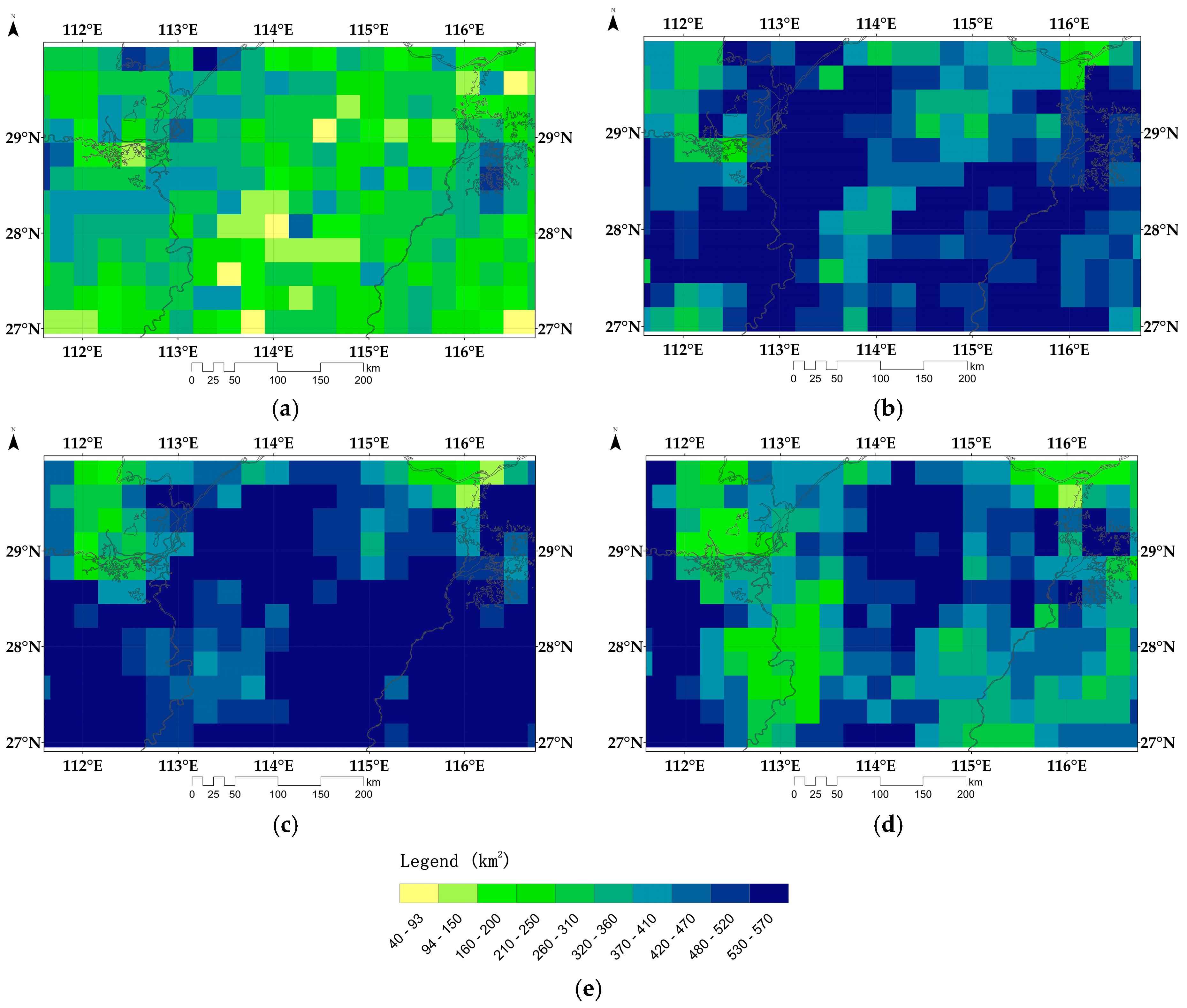
5.3. Observation of WSS over the Poyang Lake and Dongting Lake Floodplains

The Poyang Lake and Dongting Lake floodplains are in the same climate zone and are influenced by the same monsoon system, thus the frequencies associated with the surface signal that are identified for Poyang Lake can be directly applied in the Dongting Lake floodplain. According to the local hydrologic records, During April and May 2010, heavy rainfall in these two floodplains led to river stages in these two floodplains higher than the warning level, while in normal years, there is no flooding during this period. We calculated the WSS area of these two floodplains in this period of 2010 (Figure 11) and 2011 (Figure 12), respectively. The extension of WSS area in these two floodplains shows clear difference in 2010 and 2011. Large flooded area, i.e., large WSS area, can be observed in 2010, which lasts almost one month from 23 April to 25 May. In 2011, however, large WSS area is primarily observed upstream of these two floodplains (i.e., south part of the southern floodplains) and the mountain area between these two floodplains, because rainy season starts in April and monsoon system brings rainfall from south to north. This difference agrees very well with the local hydrologic and meteorological records.

6. Discussion

TSAP requires two important assumptions. One is the physical assumption that is the characteristic time scales of soil moisture, hydrometeors (precipitation as an indicator in this case), observation gaps and errors are different and distinguishable. The other is the mathematical assumption that if a signal consists of component signals and can be represented by linear and product operations, the characteristic frequency range of component signals can be identified in the power spectrum of the mixed signal. Based on these assumptions, we can analyze and understand component contributions in the power spectrum of 37 GHz PDBT time series. For example, the large peaks with periods between six and nine days in the power spectrum at two sample pixels (Figure 3) are definitely not due to atmospheric or surface signal. By analyzing the power spectrum of a synthetic signal (Figure 4) generated with the numerical model (Equation (9)) and the square wave (Equation (10)), we concluded that the extreme peak values are due to a linear combination of two square waves, which lead to these extreme-low but non-zero values in the PDBT time series (Figure 1). The estimated duration of consecutive gaps from power spectrum analysis also agrees with the orbit and scanning configuration of SSM/I [1]. This analysis clearly supports the mathematical assumption and helps interpret the spectral range of atmospheric signal in Figure 9. In the power spectrum at both sample pixels (Figure 3), we also noticed many side lobe peaks present around the components associated with the two square waves. Thus, to identify the spectral features of the surface signal, only the main lobe peaks in the power spectrum of PDBT time series were used (Figure 9).

Time series of rain-gauge data were used to reveal the characteristic frequency range of the atmospheric signal, since the occurrence of precipitation is related to large scale clouds and high water depth of hydrometeor [62]. We found clear spectral features in the power spectrum of a PDBT time series, which can be related to surface and atmospheric signals in the PDBT time series (Figure 9). The seasonal changes in soil moisture can be clearly observed in the power spectrum of PDBT time series, especially for crop land (Figure 3 and Figure 9). The shortest seasonal changes have a period of 73 days, which is comparable with the time scale of field-measured soil moisture according to [46]. The amplitudes of components in the spectral range of the atmospheric signal are much smaller than those of components representing the seasonal changes in soil moisture (Figure 9). This means that surface signal mainly controls the variations in the PDBT time series, while the atmosphere signal causes perturbations. This conclusion agrees with the physical characteristics of 37 GHz microwave, which is sensitive to surface wetness and influenced mainly by the absorption of hydrometeors. Although the spatial resolution at frequencies higher than 37 GHz can be better, e.g., at 85 GHz, the scattering of hydrometeors will be more significant [11], which causes much larger variation in the atmospheric signal. Thus, PDBT at 37 GHz is the trade-off between spatial resolution and atmosphere influence to detect surface wetness. We also noticed some short-term periodic variations in Figure 9 (as shown in Table 1), whose harmonic components have very small variations in the power spectrum of precipitation time series (Figure 8). Since the PDBT time series is mainly controlled by soil moisture, we can class these short-term periodic variations into the surface signal. The analysis on the spectral features of component signals in the PDBT time series supports our physical assumption.

The performance of the modified boxcar filter (Figure 5) shows that the filter transfer function at higher frequencies is rather smooth, which may retain part of surface and atmospheric signal, i.e., the components in the lower frequency range. We filtered out the short-term components with periods less than 20 days, as shown by the transfer function of the modified boxcar filter. The performance of the HANTS algorithm is controlled by the quality of input data, i.e., the number of reliable observations in clear days. Gaps lead to smaller number of observations and increase the difficulty of reconstructing the surface signal in the presence of extensive and persistent cloud cover. As discussed in [15], long-term high cloud cover in winter does not lead to precipitations but does attenuate the PDBT values. This may have an impact on the identification of atmospheric signal using rain-gauge data as done in our study. Thus, in the future, we will explore how to reduce the gap size by merging multi-sources data, e.g., AMSR-E and SSM/I and to combine satellite data products on precipitable water and cloud cover. In this case the application of TSAP reduced the range in daily PDBT in the lake–land boundary region from 42 K to 25 K as expected in inundated areas according to [30].

7. Conclusions

In this paper, we developed a new method, named Time Series Analysis Procedure (TSAP), to remove the daily atmospheric influence on daily 37 GHz PDBT time series and the occurrence of observation gaps and errors in this time series. Unlike other traditional methods, this method is based on the power spectrum analysis of daily PDBT time series with Discrete Fourier Transform (DFT), since the characteristic frequency range of component signals can be revealed in the power spectrum of a mixed time series. The daily 37 GHz PDBT time series is a combination of surface signal (including surface emittance and vegetation attenuation), atmospheric signal (including atmosphere emittance and attenuation, mainly from hydrometeors), observation gaps and errors. The characteristic time scale, i.e., correlation in time, of soil moisture and precipitation is very different and distinguishable, thus the seasonal changes in soil moisture can be clearly observed in the power spectrum of PDBT time series observed from SSM/I. We also found that the consecutive gaps and periodic components in observation errors introduce extreme peaks in the very high frequency spectral range. Two different filter methods were applied to remove them: observations gaps and errors were filtered out by a modified boxcar filter; and the atmospherics signal was removed by reconstructing the surface signal using the Harmonic Analysis of Time Series (HANTS) algorithm. The harmonic components due to the surface signal was separated from those due to the atmospheric signal, with the help of precipitation time series, applied as indicator of the temporal variability of atmospheric water, which has an influence on PDBT observations. The performance of the modified boxcar filter is mainly controlled by the gap size according to the Nyquist theorem. Overall, the modified boxcar filter reduces the noise level in raw PDBT time series significantly and the HANTS algorithm mitigates the impact on sample largely attenuated by the atmosphere. After TSAP, the PDBT range of the lake–land boundary region is closer to the observed range in other large flooded area, i.e., Pantanal. From the validation in Poyang Lake area, we found that TSAP is beneficial when using daily pixel-wise observations of PDBT at 37 GHz. The WSS area retrieved from the PDBT includes lake area, wet land and water saturated soil. When using the values reconstructed by HANTS in TSAP, the error of estimation is reduced from 49% to 22% and the retrieved WSS area is close to or larger than lake area observed from MODIS and ASAR, while the WSS area retrieved from raw PDBT is much less than lake area. The evolution of WSS area in the Poyang Lake and Dongting Lake floodplains clearly show the annual difference and the development of flooding.

References

1. Hollinger, J.P.; Peirce, J.L.; Poe, G.A. SSM/I instrument evaluation. IEEE Trans. Geosci. Remote Sens. 1990, 28, 781–790. [Google Scholar] [CrossRef]
2. Kawanishi, T.; Sezai, T.; Ito, Y.; Imaoka, K.; Takeshima, T.; Ishido, Y.; Shibata, A.; Miura, M.; Inahata, H.; Spencer, R.W. The advanced microwave scanning radiometer for the earth observing system (AMSR-E), NASDA’s contribution to the EOS for global energy and water cycle studies. IEEE Trans. Geosci. Remote Sens. 2003, 41, 184–194. [Google Scholar] [CrossRef]
3. Armstrong, R.; Knowles, K.; Brodzik, M.; Hardman, M.A. DMSP SSM/I-SSMIS Pathfinder Daily EASE-Grid Brightness Temperatures; Version 2; NASA DAAC at the National Snow and ICE Data Center: Boulder, CO, USA, 1998. [Google Scholar]
4. Knowles, K.; Savoie, M.; Armstrong, R.; Brodzik, M. AMSR-E/Aqua Daily EASE-Grid Brightness Temperatures; NASA DAAC at the National Snow and ICE Data Center: Boulder, CO, USA, 2006. [Google Scholar]
5. Prigent, C.; Rossow, W.B.; Matthews, E. Microwave land surface emissivities estimated from SSM/I observations. J. Geophys. Res. Atmos. 1997, 102, 21867–21890. [Google Scholar] [CrossRef]
6. Poe, G.A. Optimum interpolation of imaging microwave radiometer data. IEEE Trans. Geosci. Remote Sens. 1990, 28, 800–810. [Google Scholar] [CrossRef]
7. Poe, G.A.; Conway, R.W. A study of the geolocation errors of the special sensor microwave/imager (SSM/I). IEEE Trans. Geosci. Remote Sens. 1990, 28, 791–799. [Google Scholar] [CrossRef]
8. Ferraro, R.R.; Marks, G.F. The development of SSM/I rain-rate retrieval algorithms using ground-based radar measurements. J. Atmos. Ocean. Technol. 1995, 12, 755–770. [Google Scholar] [CrossRef]
9. Kummerow, C.; Olson, W.S.; Giglio, L. A simplified scheme for obtaining precipitation and vertical hydrometeor profiles from passive microwave sensors. IEEE Trans. Geosci. Remote Sens. 1996, 34, 1213–1232. [Google Scholar] [CrossRef]
10. Wentz, F.J. SSM/I Version-7 Calibration Report; Remote Sensing Systems: Santa Rosa, CA, USA, 2013; p. 46. [Google Scholar]
11. Ulaby, F.T.; Moore, R.K.; Fung, A.K. Microwave Remote Sensing: Active and Passive; Addison-Wesley Pub. Co., Advanced Book Program/World Science Division: Reading, MA, USA, 1981. [Google Scholar]
12. Prigent, C.; Aires, F.; Rossow, W.; Matthews, E. Joint characterization of the vegetation by satellite observations from visible to microwave wavelengths: A sensitivity analysis. Characterization of the vegetation by satellite observations. J. Geophys. Res. Atmos. 2001, 106, 20665–20685. [Google Scholar] [CrossRef]
13. Prigent, C.; Matthews, E.; Aires, F.; Rossow, W.B. Remote sensing of global wetland dynamics with multiple satellite data sets. Geophys. Res. Lett. 2001, 28, 4631–4634. [Google Scholar] [CrossRef]
14. Prigent, C.; Papa, F.; Aires, F.; Rossow, W.; Matthews, E. Global inundation dynamics inferred from multiple satellite observations, 1993–2000. J. Geophys. Res. Atmos. 2007, 112, D12107. [Google Scholar] [CrossRef]
15. Shang, H.; Jia, J.; Menenti, M. Analyzing the inundation pattern of the Poyang Lake floodplain by passive microwave data. J. Hydrometeorol. 2015, 16, 652–667. [Google Scholar] [CrossRef]
16. Kerr, Y.H.; Waldteufel, P.; Wigneron, J.-P.; Martinuzzi, J.; Font, J.; Berger, M. Soil moisture retrieval from space: The soil moisture and ocean salinity (SMOS) mission. IEEE Trans. Geosci. Remote Sens. 2001, 39, 1729–1735. [Google Scholar] [CrossRef]
17. Njoku, E.G.; Jackson, T.J.; Lakshmi, V.; Chan, T.K.; Nghiem, S.V. Soil moisture retrieval from AMSR-E. IEEE Trans. Geosci. Remote Sens. 2003, 41, 215–229. [Google Scholar] [CrossRef]
18. O’Neill, P.E.; Jackson, T.J.; Chauhan, N.S.; Seyfried, M.S. Microwave soil moisture estimation in humid and semiarid watersheds. Adv. Space Res. 1993, 13, 115–118. [Google Scholar] [CrossRef]
19. Paloscia, S.; Macelloni, G.; Santi, E.; Koike, T. A multi-frequency algorithm for the retrieval of soil moisture on a large scale using microwave data from SMMR and SSM/I satellites. IEEE Trans. Geosci. Remote Sens. 2001, 39, 1655–1661. [Google Scholar] [CrossRef]
20. Wang, J.R.; Choudhury, B.J. Remote sensing of soil moisture content over bare field at 1.4 GHz frequency. J. Geophys. Res. 1981, 86, 5277–5282. [Google Scholar] [CrossRef]
21. Choudhury, B.J. Monitoring global land surface using nimbus-7 37 GHz data. Theory and examples. Int. J. Remote Sens. 1989, 10, 1579–1605. [Google Scholar] [CrossRef]
22. Giddings, L.; Choudhury, B.J. Observation of hydrological features with nimbus-7 37 GHz data, applied to South America. Int. J. Remote Sens. 1989, 10, 1673–1686. [Google Scholar] [CrossRef]
23. Hamilton, S.K.; Sippel, S.J.; Melack, J.M. Inundation patterns in the Pantanal wetland of South America determined from passive microwave remote sensing. Arch. Hydrobiol. 1996, 137, 1–23. [Google Scholar]
24. Hamilton, S.K.; Sippel, S.J.; Melack, J.M. Comparison of inundation patterns among major South American floodplains. J. Geophys. Res. D Atmos. 2002, 107, 8038. [Google Scholar] [CrossRef]
25. Hamilton, S.K.; Sippel, S.J.; Melack, J.M. Seasonal inundation patterns in two large savanna floodplains of South America: The llanos De Moxos (Bolivia) and the llanos Del Orinoco (Venezuela and Colombia). Hydrolog. Process. 2004, 18, 2103–2116. [Google Scholar] [CrossRef]
26. Sippel, S.J.; Hamilton, S.K.; Melack, J.M.; Choudhury, B.J. Determination of inundation area in the amazon river floodplain using the SMMR 37 Ghz polarization difference. Remote Sens. Environ. 1994, 48, 70–76. [Google Scholar] [CrossRef]
27. Sippel, S.J.; Hamilton, S.K.; Melack, J.M.; Novo, E.M.M. Passive microwave observations of inundation area and the area/stage relation in the amazon river floodplain. Int. J. Remote Sens. 1998, 19, 3055–3074. [Google Scholar] [CrossRef]
28. Tanaka, M.; Sugimura, T.; Tanaka, S.; Tamai, N. Flood–drought cycle of Tonle Sap and Mekong delta area observed by DMSP-SSM/I. Int. J. Remote Sens. 2003, 24, 1487–1504. [Google Scholar] [CrossRef]
29. Choudhury, B.J.; Major, E.R.; Smith, E.A.; Becker, F. Atmospheric effects on SMMR and SSM/I 37 GHz polarization difference over the sahel. Int. J. Remote Sens. 1992, 13, 3443–3463. [Google Scholar] [CrossRef]
30. Choudhury, B.J. Passive microwave remote sensing contribution to hydrological variables. In Land Surface-Atmosphere Interactions for Climate Modeling; Springer: Dordrecht, The Netherlands, 1991; pp. 63–84. [Google Scholar]
31. Rossow, W.B.; Schiffer, R.A. Advances in understanding clouds from ISCCP. Bull. Am. Meteorol. Soc. 1999, 80, 2261. [Google Scholar] [CrossRef]
32. Aires, F.; Prigent, C.; Rossow, W.; Rothstein, M.; Hansen, J.E. A new neural network approach including first-guess for retrieval of atmospheric water vapor, cloud liquid water path, surface temperature and emissivities over land from satellite microwave observations. J. Geophys. Res. 2001, 106, 14887–14907. [Google Scholar] [CrossRef]
33. Behrangi, A.; Guan, B.; Neiman, P.J.; Schreier, M.; Lambrigtsen, B. On the quantification of atmospheric rivers precipitation from space: Composite assessments and case studies over the eastern North Pacific Ocean and the western united states. J. Hydrometeorol. 2016, 17, 369–382. [Google Scholar] [CrossRef]
34. Boukabara, S.-A.; Garrett, K.; Chen, W. Global coverage of total precipitable water using a microwave variational algorithm. IEEE Trans. Geosci. Remote Sens. 2010, 48, 3608–3621. [Google Scholar] [CrossRef]
35. Reale, A.; Chalfant, M.; Allegrino, A.; Tiley, F.; Gerguson, M.; Pettey, M. Advanced-TOVS (ATOVS) sounding products from NOAA polar orbiting environmental satellites. In Proceedings of the 12th Conference on Satellite Meteorology and Oceanography, Long Beach, CA, USA, 9–13 February 2003.
36. Agrawal, R.; Faloutsos, C.; Swami, A. Efficient Similarity Search in Sequence Databases; Springer: Berlin/Heidelberg, Germany, 1993. [Google Scholar]
37. Keogh, E.; Chakrabarti, K.; Pazzani, M.; Mehrotra, S. Dimensionality reduction for fast similarity search in large time series databases. Knowl. Inf. Syst. 2001, 3, 263–286. [Google Scholar] [CrossRef]
38. Lin, R.; King-lp, A.; Shim, H.S.S.K. Fast similarity search in the presence of noise, scaling, and translation in time-series databases. In Proceedings of the 21th International Conference on Very Large Data Bases, Zurich, Switzerland, 9–13 September 1995; pp. 490–501.
39. Mörchen, F. Time Series Feature Extraction for Data Mining Using DWT and DFT; University of Marburg: Marburg, Germany, 2003. [Google Scholar]
40. Wu, Y.-L.; Agrawal, D.; El Abbadi, A. A comparison of DFT and DWT based similarity search in time-series databases. In Proceedings of the Ninth International Conference on Information and Knowledge Management, McLean, VA, USA, 6–11 November 2000; pp. 488–495.
41. Harris, F.J. On the use of windows for harmonic analysis with the Discrete Fourier Transform. Proc. IEEE 1978, 66, 51–83. [Google Scholar] [CrossRef]
42. Nerem, R.; Chambers, D.; Leuliette, E.; Mitchum, G.; Giese, B. Variations in global mean sea level associated with the 1997–1998 Enso event: Implications for measuring long term sea level change. Geophys. Res. Lett. 1999, 26, 3005–3008. [Google Scholar] [CrossRef]
43. Entin, J.K.; Robock, A.; Vinnikov, K.Y.; Hollinger, S.E.; Liu, S.; Namkhai, A. Temporal and spatial scales of observed soil moisture variations in the extratropics. J. Geophys. Res. 2000, 105, 11865–11877. [Google Scholar] [CrossRef]
44. Skøien, J.O.; Blöschl, G.; Western, A. Characteristic space scales and timescales in hydrology. Water Resour. Res. 2003, 39, 1304. [Google Scholar] [CrossRef]
45. Vachaud, G.; Passerat de Silans, A.; Balabanis, P.; Vauclin, M. Temporal stability of spatially measured soil water probability density function. Soil Sci. Soc. Am. J. 1985, 49, 822–828. [Google Scholar] [CrossRef]
46. Vinnikov, K.Y.; Robock, A.; Speranskaya, N.A.; Schlosser, C.A. Scales of temporal and spatial variability of midlatitude soil moisture. J. Geophys. Res. Atmos. 1996, 101, 7163–7174. [Google Scholar] [CrossRef]
47. Wilson, D.J.; Western, A.W.; Grayson, R.B. Identifying and quantifying sources of variability in temporal and spatial soil moisture observations. Water Resour. Res. 2004, 40, W02507. [Google Scholar] [CrossRef]
48. D’Odorico, P.; Rodrı́guez-Iturbe, I. Space-time self-organization of mesoscale rainfall and soil moisture. Adv. Water Resour. 2000, 23, 349–357. [Google Scholar] [CrossRef]
49. Menenti, M.; Azzali, S.; Verhoef, W.; van Swol, R. Mapping agro-ecological zones and time lag in vegetation growth by means of fourier analysis of time series of NDVI images. Adv. Space Res. 1993, 13, 233–237. [Google Scholar] [CrossRef]
50. Jia, L.; Shang, H.; Hu, G.; Menenti, M. Phenological response of vegetation to upstream river flow in the Heihe river basin by time series analysis of MODIS data. Hydrol. Earth Syst. Sci. 2011, 15, 1047–1064. [Google Scholar] [CrossRef] [Green Version]
51. Roerink, G.J.; Menenti, M.; Soepboer, W.; Su, Z. Assessment of climate impact on vegetation dynamics by using remote sensing. Phys. Chem. Earth 2003, 28, 103–109. [Google Scholar] [CrossRef]
52. Roerink, G.J.; Menenti, M.; Verhoef, W. Reconstructing cloudfree NDVI composites using Fourier analysis of time series. Int. J. Remote Sens. 2000, 21, 1911–1917. [Google Scholar] [CrossRef]
53. Verhoef, W. Application of harmonic analysis of NDVI time series (HANTS). In Fourier Analysis of Temporal NDVI in the Souther African and American Continents; Azzali, S., Menenti, M., Eds.; DLO Winand Staring Centre: Wageningen, The Netherlands, 1996; pp. 19–24. [Google Scholar]
54. Cooley, J.W.; Lewis, P.A.; Welch, P.D. Application of the fast Fourier transform to computation of Fourier integrals, Fourier series, and convolution integrals. IEEE Trans. Audio Electroacoust. 1967, 15, 79–84. [Google Scholar] [CrossRef]
55. Cooley, J.W.; Tukey, J.W. An algorithm for the machine calculation of complex Fourier series. Math. Comput. 1965, 19, 297–301. [Google Scholar] [CrossRef]
56. Singleton, R.C. An algorithm for computing the mixed radix fast Fourier transform. IEEE Trans. Audio Electroacoust. 1969, 17, 93–103. [Google Scholar] [CrossRef]
57. Project, B.M.; Erdélyi, A.; Bateman, H. Tables of Integral Transforms: Based in Part on Notes Left by Harry Bateman and Compiled by the Staff of the Bateman Manuscript Project; McGraw-Hill: New York, NY, USA, 1954. [Google Scholar]
58. Yésou, H.; Claire, H.; Xijun, L.; Stéphane, A.; Jiren, L.; Sylviane, D.; Muriel, B.-N.; Xiaoling, C.; Shifeng, H.; Burnham, J.; et al. Nine years of water resources monitoring over the middle reaches of the Yangtze river, with ENVISAT, MODIS, Beijing-1 time series, altimetric data and field measurements. Lakes Reserv. Res. Manag. 2011, 16, 231–247. [Google Scholar]
59. Thompson, A.R.; Moran, J.M.; Swenson, G.W., Jr. Interferometry and Synthesis in Radio Astronomy; John Wiley & Sons: Weinheim, Germany, 2008. [Google Scholar]
60. Czekala, H.; Havemann, S.; Schmidt, K.; Rother, T.; Simmer, C. Comparison of microwave radiative transfer calculations obtained with three different approximations of hydrometeor shape. J. Quant. Spectrosc. Radiat. Transf. 1999, 63, 545–558. [Google Scholar] [CrossRef]
61. Gerek, Ö.N.; Yardimci, Y. Equiripple fir filter design by the FFT algorithm. IEEE Signal Process. Mag. 1997, 14, 60–64. [Google Scholar]
62. Richards, F.; Arkin, P. On the relationship between satellite-observed cloud cover and precipitation. Mon. Weather Rev. 1981, 109, 1081–1093. [Google Scholar] [CrossRef]
Figure 1. Raw space-borne Polarization Difference Brightness Temperature (PDBT) time series at two sample pixels from 1998 to 2007. All gaps are assigned a value of 0. The dominant land cover in the 1st sample pixel (a) is farm land, centered at 28.603°N and 115.835°E. The dominant land cover in the 2nd sample pixel (b) is open water and wet land, centered at 29.049°N and 116.356°E. Their locations are shown in Figure 2. Date format: yyyy/mm/dd.
Remotesensing 08 00970 g001
Figure 2. Location of the first (numbered with 1) and the second (numbered with 2) sample pixel in the Poyang Lake floodplain, China.
Remotesensing 08 00970 g002
Figure 3. Power spectrum of the space-borne Polarization Difference Brightness Temperature (PDBT) time series for the: 1st (a); and 2nd (b) example pixels from 1998 to 2007. The dominant land cover of the 1st sample pixel is farm land, centered at 28.603°N and 115.835°E. The dominant land cover of the 2nd sample pixel is open water and wet land, centered at 29.049°N and 116.356°E. FFT: Fast Fourier Transform
Remotesensing 08 00970 g003
Figure 4. Power spectrum of the square wave in Equation (8) with L = 8 days (a); and power spectrum of the sum of two square waves with L = 7 days and L = 8 days with unit amplitude (b).
Remotesensing 08 00970 g004aRemotesensing 08 00970 g004b
Figure 5. The Normalized Difference (ND) between amplitudes of harmonic components in Equation (13) and their filtered amplitudes for 10-year time series.
Remotesensing 08 00970 g005
Figure 6. The Polarization Difference Brightness Temperature (PDBT) time series after applying the boxcar filter, its HANTS reconstruction and the daily cumulated precipitation from 1998 to 2007 for: the 1st sample pixel (a); and the 2nd sample pixel (b). Date format: yyyy/mm/dd.
Remotesensing 08 00970 g006aRemotesensing 08 00970 g006b
Figure 7. The cumulated power spectrum of 10-year precipitation time series for: the 1st sample pixel (a); and the 2nd sample pixel (b).
Remotesensing 08 00970 g007
Figure 8. Harmonic components with peak power in the power spectrum of rain-gauge time series in the period range [20 days, 182 days] for both the 1st and the 2nd sample pixels.
Remotesensing 08 00970 g008
Figure 9. Harmonic components with main lobe peaks in the power spectrum of the PDBT time series in the period range [20 days, 182 days] for both the 1st and the 2nd sample pixels. The main lobe peaks are defined as the peak values in the upper envelope of the power spectrum.
Remotesensing 08 00970 g009
Figure 10. The retrieved Poyang lake area from original PDBT data, filtered PDBT and HANTS reconstructed PDBT, compared with lake area observed with the MODIS and ASAR by [58].
Remotesensing 08 00970 g010
Figure 11. The Water Saturated Surface (WSS) area within each 25 km × 25 km pixel on: 7 April (a); 23 April (b); 9 May (c); and 25 May (d) of 2010 in the Dongting Lake and Poyang Lake floodplains; (e) the legend of images from (a) to (d). Dongting Lake is located on the left side and Poyang Lake is located on the right side, with their boundary lines shown in each image.
Remotesensing 08 00970 g011
Figure 12. the WSS area within each 25 km × 25 km pixel on: 7 April (a); 23 April (b); 9 May (c); and 25 May (d) of 2011 in the Dongting Lake and Poyang Lake floodplains; (e) the legend of images from (a) to (d). Dongting Lake is located on the left side and Poyang Lake is located on the right side, with their boundary lines shown in each image.
Remotesensing 08 00970 g012