Aerosol Retrievals from CALIPSO Lidar Ocean Surface Returns

Abstract

This paper describes approaches to retrieve important aerosol results from the strong lidar return signals that are received by the space-borne CALIPSO lidar system after reflecting off-ocean surfaces. Relations, from which the theoretically expected values of area under ocean surface returns can be computed, are presented. A detailed description of the lidar system response to the ocean surface returns and the processes of sampling and averaging of lidar return signals are provided. An effective technique that reconstructs the lidar response to surface returns—starting from down-linked samples—and calculates the area under it, has been developed and described. The calculated area values are validated after comparing them to their theoretically predicted counterpart values. Methods to retrieve aerosol optical depths (AODs) from these calculated areas are described and retrieval results are presented, including retrieval comparison with independent AOD measurements made by an airborne High Spectral Resolution Lidar (HSRL) that yielded quite good agreement. Techniques and results are also presented on using the spectral ratios of the surface response areas to determine spectral ratios of aerosol round-trip transmission and AOD spectral difference, without need of a specific/accurate ocean-surface reflectance model.

1. Introduction

LIght Detection And Ranging (lidar) is an optical remote sensing technology which is very often used in the study of atmospheric aerosols. Similar in concept to radar, lidar emits highly coherent, ultra-short laser pulses at wavelengths which are comparable to the dimensions of atmospheric aerosol particles. This permits lidar pulses to physically interact fairly strongly with aerosols such as dust, pollen, smoke, etc. The inability of in situ instruments to make aerosol measurements on a global scale and the high variability of both spatial and temporal distributions of tropospheric aerosols drive the necessity for space-borne observations.

Cloud-Aerosol Lidar and Infrared Pathfinder Satellite Observation (CALIPSO) is a satellite lidar system that was launched by NASA on 28 April 2006 to improve our knowledge and understanding of the roles played by cloud and aerosol particles on Earth’s climate change. Being the first space-borne lidar dedicated to the study of aerosols, CALIPSO can make observations and measurements on a global scale that help provide insight into the factors that regulate Earth’s radiation budget. The principal goals of the CALIPSO mission are to provide global, vertically resolved aerosol microphysical properties and spatial distributions, perform height-resolved discrimination of aerosols into several types, to provide vertical layers of single and multi-layer transmissive clouds and to determine vertical distributions of cloud ice and water [1,2,3].

Laser pulses transmitted from the lidar system into the atmosphere are reflected back to the system as a result of back-scattering by various particles present in the propagation path of the pulse. Backscatter of the laser pulses also occurs from hard targets such as land and ocean surfaces which result in what are referred to as “surface returns.” Surface returns are expected to be much stronger than the atmospheric returns and carry in them qualitative and quantitative factors about the material medium present in the atmosphere through which the transmitted lidar pulses have travelled. This paper includes an in-depth analysis of surface returns from ocean surfaces and presents ways to retrieve optical depths from these returns. It is a summary, with some revisions and additions, of the work completed by the first author for his M.S. thesis [4].

2. Materials and Methods

2.1. Low-Pass Filter

The lidar system on board CALIPSO is called Cloud-Aerosol LIdar with Orthogonal Polarization (CALIOP). CALIOP employs a third-order low-pass Bessel filter with a bandwidth ~2.44 MHz, as a part of its post-detection electronics following the PMT detector for the 532 nm channel [5,6,7]. Similar post-detection electronics, with the same low-pass filter, follows the avalanche photodiode (APD) detector for the 1064 nm channel. A very important feature of this Bessel low-pass filter (LPF) is that for a pulse return signal (as occurs from a hard-target reflection) it preserves the area under the pulse. Thus, if a narrow pulse enters this filter, its peak amplitude is reduced but the pulse is stretched in time so as to preserve the area under the original narrow pulse. This enables accurate capture of the hard target ocean surface response at the 10 MHz digitation rate of the digitizers following the LPF. For a Dirac delta function time input to the LPF, the convolution integral of the delta function input convolved with the LPF output-to-input transfer function yields the transient output known as the Impulse Response Function (IRF). If the input is not a delta function, but a short pulse compared to the IRF response time, as is the case for the short-duration transmitted lidar pulse (~20 ns), the convolution with the LPF transfer function still yields the ideal IRF to a very close approximation (simulations showed that the impulse response of the LPF for an input pulse of duration of the transmitted lidar pulse yielded a response within ~0.1% of the ideal IRF). As with any linear time-invariant (LTI) system, the third-order Bessel filter can be completely characterized by its IRF.

Impulse response measurements were made on flight hardware replicas of the CALIOP detector and post-detection electronics where the detector was exposed to optical pulses of about 20 ns duration to mimic the laser pulse transmitted by CALIOP [5]. The measured impulse response, averaged over many measurements, scaled to unity area is shown in Figure 1 [5]. The circles are the digitized samples (at the 10 MHz sample rate), and the solid line is an analytical best-fit using a hyperbolic tangent for the rising part of the pulse and a Gaussian curve for the falling part [5].

As the transfer functions of Bessel filters are very well characterized, using the control system tool-box of MATLAB, the ideal impulse response shape was generated (assuming the ~2.44 MHz bandwidth exhibited by the measured response). To compare the two impulse responses (lab measured and MATLAB generated), they are scaled to have the same area (unity) and are plotted in Figure 2. It can be concluded that, within a very close approximation, the impulse response of the CALIOP receiver electronics does indeed replicate the theoretical IRF for a third-order Bessel low-pass transfer function (and the areas found using either impulse response curve to obtain areas under CALIPSO ocean surface returns were found to be the same within ~1%). For the work reported in this paper, the impulse response is assumed to be the fit made to the lab measurements (solid curve in Figure 1). It should be noted that should subsequent investigations determine a somewhat more accurate model for the impulse response, the difference in determining the area under the lidar surface response (SR) with the improved model would only be a small, fractionally fixed bias that could easily be corrected.

2.2. Area under Surface Return Pulse

The lidar equation for the instantaneous return signal from a distributed source such as the atmosphere can be expressed as [8]

$${\mathrm{V}}_{\mathsf{\lambda }}\left(\mathrm{z}\right)=\frac{{\mathrm{CE}}_{\mathrm{o}}{\mathsf{\beta }}_{\mathsf{\lambda }}\left(\mathrm{z}\right){\mathrm{T}}_{\mathsf{\lambda }}^2\left(\mathrm{z}\right)}{{\mathrm{z}}^2},$$

(1)

where V_λ represents the lidar return signal from range z expressed as a voltage level, z is the range from the lidar increasing downward towards the Earth’s surface, E_o represents the transmitted pulse energy, ${\mathsf{\beta }}_{\mathsf{\lambda }}$ represents the backscatter coefficient at wavelength λ expressed in units of m⁻¹·sr⁻¹, ${\mathrm{T}}_{\mathsf{\lambda }}^2$(z) is the atmospheric round-trip path transmittance to and from range z at wavelength λ and C is the calibration constant. Return signals from the atmosphere are mostly slowly varying and have longer durations than the impulse response of the LPF. Hence the LPF has little effect on the atmospheric returns and the output of the LPF can be well approximated by Equation (1). However, the lidar response to surface returns V_λs, before entering the LPF, is a pulse which is a replica of the originally transmitted Gaussian-shaped lidar pulse of duration t_p (t_p ≈ 20 ns). As this pulse is much narrower than the impulse response of the LPF, the output of the filter can be assumed to be the ideal impulse response IRF of the filter itself. Hence, the time integrated output of the LPF “V_{λS LPF}” for the surface return response “V_λs” is given by

$$\underset{0}{\overset{{\mathrm{t}}_{\mathrm{p}}}{{\displaystyle \int }}}{\mathrm{V}}_{\mathsf{\lambda }\mathrm{S}}\mathrm{dt}=\underset{0}{\overset{{\mathrm{t}}_{\mathrm{p}}^{\prime }}{{\displaystyle \int }}}{\mathrm{V}}_{\mathsf{\lambda }\mathrm{S}\mathrm{LPF}}\left(\mathrm{t}\right)\mathrm{dt},$$

(2)

where t_p’ is the duration of the output of the LPF (the impulse response duration). Defining “z_s” to be range to the surface, from Equations (1) and (2) we have

$$\underset{0}{\overset{{\mathrm{t}}_{\mathrm{p}}}{{\displaystyle \int }}}{\mathrm{V}}_{\mathsf{\lambda }\mathrm{S}}\mathrm{dt}=\frac{{\mathrm{C}}_{\mathsf{\lambda }}{\mathrm{E}}_0{\mathrm{T}}^2\left({\mathrm{z}}_{\mathrm{s}}\right)}{{\mathrm{z}}_{\mathrm{S}}^2}\underset{0}{\overset{{\mathrm{t}}_{\mathrm{p}}^{\prime }}{{\displaystyle \int }}}\mathsf{\beta }\left(\mathrm{t}\right)\mathrm{dt},$$

(3)

Taking the round-trip propagation time t into account, dt can be written as $\frac{2\mathrm{dz}}{\mathrm{c}}$ so that

$$\underset{0}{\overset{{\mathrm{t}}_{\mathrm{p}}}{{\displaystyle \int }}}{\mathrm{V}}_{\mathsf{\lambda }\mathrm{S}}\mathrm{dt}=\frac{2{\mathrm{E}}_0{\mathrm{T}}^2\left({\mathrm{z}}_{\mathrm{s}}\right){\mathrm{C}}_{\mathsf{\lambda }}}{{\mathrm{cz}}_{\mathrm{S}}^2}\underset{0}{\overset{{\mathrm{z}}^{\prime }}{{\displaystyle \int }}}\mathsf{\beta }\left(\mathrm{z}\right)\mathrm{dz},$$

(4)

For a hard target we replace ${{\displaystyle \int }}_0^{{\mathrm{z}}^{\prime }}\mathsf{\beta }\left(\mathrm{z}\right)\mathrm{dz}$ with R_λ, the retro or backscatter reflectance (sr⁻¹) of the surface. Hence, the expected surface return area, A_LPF, after being normalized by the calibration constant, peak energy and range squared (just as the lidar equation, Equation (1), is normalized for the CALIPSO level 1 data product) is given by

$${\mathrm{A}}_{\mathrm{LPF}}=\frac{2{\mathrm{T}}^2\left({\mathrm{z}}_{\mathrm{s}}\right){\mathrm{R}}_{\mathsf{\lambda }}}{\mathrm{c}},$$

(5)

The area under the surface-return response pulse thus depends on the product of the surface reflectance and total round-trip transmission. In other words, the response of the lidar receiver to ocean-surface return signals is a scaled version of the impulse response shown in Figure 1, and the magnitude of the scaling depends on the amount of atmospheric attenuation and the reflectance value of the ocean surface. With the normalizations, A_LPF does not actually have the units of area, but will be referred to as an area in subsequent discussions. Also, c must be evaluated in units of km/μsec (c = 0.3 km/μsec) in Equation (5) to yield A_LPF values consistent with the CALIPSO data product sample values of the surface response signals, and the A_LPF inferred from the samples, per/characterized by the similarly normalized lidar equation.

2.3. Ocean Surface Reflectance

Considerable effort ([9,10,11,12], to name a few) has been directed over the years to develop a model that can relate the surface reflectance to the surface wind speed (WS) and wave facet characteristics and accurately determine it. The ocean-surface reflectance model used in this paper was developed in [13]. This model is a revised and updated version of the model developed by Cox and Munk [9] and is presented below. In general, the ocean-surface backscatter reflectance, R_λ, units of sr⁻¹, can be modeled by

$${\mathrm{R}}_{\mathsf{\lambda }}=\left(1-\mathrm{W}\right)\times \mathrm{Retro}\_\mathrm{Fresnel}\_\mathrm{Reflectance}+\mathrm{W}\times 0.2,$$

(6)

where “W” represents the fraction of the surface covered with whitecaps and “Retro_Fresnel_Reflectance” is the Fresnel reflectance of the ocean-surface at nadir (e.g., [14]). They are given by

$$\mathrm{Whitecap}\mathrm{Fraction}=2.95\times {10}^{-6}\times {\mathrm{WindSpeed}}^{3.37},$$

(7)

$$\mathrm{Retro}\_\mathrm{Fresnel}\_\mathrm{Reflectance}=\frac{\mathrm{Fresnel}\mathrm{Coeficient}}{4\mathsf{\pi }〈\mathrm{wave}\_\mathrm{slope}{〉}^2},$$

(8)

Here, as the name suggests, “WindSpeed” refers to surface wind speed (WS). The Fresnel Coefficient (ρ) is spectrally dependent and at 532 nm and 1064 nm has estimated values of ρ₅₃₂ = 0.0205 and ρ₁₀₆₄ = 0.019 and ${〈\mathrm{wave}\_\mathrm{slope}〉}^2$ represents the variance of the distribution of wave slopes and is given by

$$〈\mathrm{wave}\_\mathrm{slope}{〉}^2=-0.006+7.95\times {10}^{-3}\times \mathrm{WindSpeed},$$

(9)

Thus, with known surface wind speeds (WS), the terms in Equations (7)–(9) can be calculated and the final reflectance can be determined using Equation (6). Figure 3 shows the variation of the ocean-surface reflectance at 532 nm wavelength, R₅₃₂, with surface wind speed (WS). As the reflectance rises sharply at low wind speeds (WS < ~3 m/s), use of the reflectance model/input WS data in estimating A_LPF must be limited to higher WS, but also be cut off at too high a wind speed where the reflectance model becomes less accurate (to be on the conservative side, analysis of CALIPSO data to retrieve A_LPF presented here has been limited to WS between ~4 m/s to ~8 m/s).

2.4. Signal Acquisition and Post-Filtering Processing

The lidar response, generated after photon detection of the received signal and post-detection amplification, is sampled and digitized after being low-pass filtered. The generated samples undergo a wavelength channel-specific averaging scheme before being down-linked from the satellite [6]. Thus, down-linked samples corresponding to ocean surface returns are the result of sampling and averaging a scaled version of the LPF’s impulse response.

2.4.1. Sampling and Generation of Down-Linked Samples

The fundamental sampling of the filter output for both wavelength channels occurs at 10 MHz frequency (consecutive samples hence separated by 0.1 μsec), insuring that samples meet the sampling theorem requirement for reconstructing the sampled signal (bandwidth of the LPF is ~2.5 MHz). Sampling at this frequency essentially means that the vertical decimation of the atmosphere is performed in such a manner that the return signal is collected every 15 m along the transmission path of the lidar pulse. Figure 4 below shows the impulse response (in solid blue) and the primary samples (shown in black) separated by 0.1 μsec. For the 532 nm channel, every down-linked sample is generated by pairing consecutive primary samples and averaging them in both value and their time instants to obtain the corresponding values for the down-linked sample. The down-linked samples are shown in red in Figure 4 and it can be observed that consecutive down-linked samples are separated by 0.2 μsec, which means that the effective vertical range resolution is reduced to 30 m for the 532 nm channel.

For the 1064 nm channel, down-linked samples are obtained after averaging consecutive primary samples in groups of four. Figure 5 describes this process by showing the original impulse response, its primary samples and the final down-linked samples. Since the 1064 nm channel requires twice the number of primary samples to be averaged to generate the down-linked sample when compared to the 532 nm channel, the total number of down-linked samples for the 1064 nm channel is half that of the 532 nm channel. However, the CALIPSO data product, from where the down-linked samples for both channels are retrieved, duplicates every down-linked sample of the 1064 nm channel and stores it beside the original sample in order to store the same number of down-linked samples for both the 1064 nm and 532 nm channels. Hence, while the 1064 nm channel-duplicated samples are separated in time by 0.2 μsec just as in the 532 nm channel, filtering out the duplicated samples leaves behind only the original samples (shown in red in Figure 5) that are separated by 0.4 μsec which corresponds to an effective vertical range resolution of 60 m. All analysis of the 1064 nm channel data was done with only the original samples after filtering out the duplicate samples.

2.4.2. Effect of Sampling Delay on Down-Linked Samples

As the primary samples are uniformly spaced with 0.1 μsec separation, the time instant of the first sample of the impulse response determines the time instances and hence the magnitudes of the remaining samples that follow. On board CALIOP, the starting sampling instant is variable (e.g., due to digitizer jitter, difference in ocean surface elevation at different locations/sea states, and imperfect pointing, position and orbit propagation knowledge on board the satellite) [7]. Thus, different lidar shots can have different starting sampling instances and hence surface samples corresponding to one lidar shot maybe “delayed” and, thus, may differ in magnitudes in comparison to samples obtained from another lidar shot. This process is depicted at 532 nm in Figure 6. Similarly, Figure 7 shows the influence of sampling delay on the magnitude of the down-linked samples for the 1064 nm channel.

The effect of sampling delay on the magnitude of down-linked samples is quite evident where it can be seen that the values of the down-linked samples change relative to one another with delay. The delay must be taken into account in estimating the SR area for any given lidar shot. That is, the impulse response model used to estimate the area must be positioned under the SR samples for a given shot for the sampling delay of that shot. The delay can be estimated by the ratio of the first to second samples for a given shot. Piecewise cubic hermite (shape preserving) interpolation was performed at both wavelengths so that for every intermediate ratio, a sampling delay is assigned. The interpolation results are shown in Figure 8. For the 532 nm channel, the remaining two samples are 0.2 µsec and 0.4 µsec away from the first sample. For the 1064 nm channel, the second sample is 0.4 µsec away from the first sample. Hence, for every lidar shot, time instances may be assigned to all the surface return samples at both wavelengths. It should be noted that, regardless of the time delay, the sum of the down-linked samples (sum value) that make up a given SR pulse is very nearly constant (within ~2%), for no noise present, and, as discussed later, can be used as a quality check to reject bad shots.

2.4.3. Down-Linked Samples

The principle data product that is down-linked from CALIPSO is the attenuated backscatter (km⁻¹·sr⁻¹), which for a range “z” is defined as

$$\mathrm{Attenuated}\mathrm{Backscatter}=\left({\mathsf{\beta }}_{\mathrm{R}}\left(\mathrm{z}\right)+{\mathsf{\beta }}_{\mathrm{a}}\left(\mathrm{z}\right)\right)\times {\mathrm{T}}_{\mathrm{R}}^2\left(\mathrm{z}\right)\times {\mathrm{T}}_{\mathrm{a}}^2\left(\mathrm{z}\right)\times {\mathrm{T}}_{\mathrm{Ozone}}^2,$$

(10)

where β_a and β_R represent the aerosol and Rayleigh components of the backscatter coefficient and T²_a, T²_R and T²_Ozone represent the aerosol, Rayleigh and ozone components of the round-trip transmission, respectively. It should be noted that the attenuated backscatter data product has been normalized to take out the lidar calibration for each wavelength, for the given lidar orbit position, as a part of CALIPSO standard data processing. For every lidar shot, the CALIPSO data product provides the attenuated backscatter for 583 altitude bins at both wavelengths. Surface returns can easily be identified (so long as the atmospheric optical depth is not too great due to clouds or optically thick aerosol layers) from amongst the 583 bins as they are significantly stronger than the atmospheric returns. The ocean surface returns were observed to be made up of three down-linked samples for the 532 nm channel, and two down-linked samples for the 1064 nm channel, and they were almost always found to lie within bins 561–565 in the data product for both channels. Figure 9 shows samples for both wavelength channels corresponding to a typical surface return signal. It should be noted that the horizontal scales are not the same for the two channels (scale for 1064 nm is double, two bin increments).

A useful parameter to assess the amount of aerosol loading in the atmosphere is the integral of the attenuated backscatter down to the surface, the total integrated attenuated backscatter (TIAB), units of sr⁻¹. Thus, if “z_s” is the range to the surface

$$\mathrm{TIAB}=\underset{0}{\overset{{\mathrm{Z}}_{\mathrm{S}}}{{\displaystyle \int }}}\left({\mathsf{\beta }}_{\mathrm{Aerosol}}+{\mathsf{\beta }}_{\mathrm{Rayleigh}}\right)\times {\mathrm{T}}_{\mathrm{Aerosol}}^2\times {\mathrm{T}}_{\mathrm{Rayleigh}}^2\times {\mathrm{T}}_{\mathrm{Ozone}}^2\mathrm{dz},$$

(11)

From its definition, TIAB is expected to increase with increasing aerosol backscatter, although if β_a(z) becomes too large, the corresponding impact on T_a²(z) will cause TIAB to decrease. Even as TIAB increases, T_a²(z) still decreases with increasing β_a (z), causing the strength of observed surface returns to generally decrease with increasing TIAB. Under very clear sky conditions (aerosol-free atmosphere) for 532 nm the TIAB reduces to

$${\mathrm{TIAB}}_{\left(\mathrm{Clear}\mathrm{sky}\right)}=\underset{0}{\overset{{\mathrm{z}}_{\mathrm{s}}}{{\displaystyle \int }}}{\mathsf{\beta }}_{\mathrm{Rayleigh}}\times {\mathrm{T}}_{\mathrm{Rayleigh}}^2\times {\mathrm{T}}_{\mathrm{Ozone}}^2\mathrm{dz},$$

(12)

Using the molecular and ozone density numbers provided in the CALIPSO data product, all the terms within the integral in Equation (12) can be computed and for the 532 nm channel the TIAB for clear sky conditions was calculated to be ~0.012. Thus, a TIAB threshold value of 0.0125 was set so that any 532 nm lidar shot having a TIAB value ≤0.0125 was assumed to have passed through an essentially aerosol-free atmosphere. The CALIPSO data product also provides, for every lidar shot, its eastward and westward wind component values (the wind information is provided from NASA’s Global Modeling and Assimilation Office (GMAO); the wind being estimated from an assimilation model). The total surface wind speed can be obtained by taking the vector sum of these components, from which the surface reflectance can be calculated using the model described earlier. Thus, every lidar shot can be associated with a TIAB and surface reflectance value.

2.5. Reconstruction of Impulse Response and Area Retrieval from Down-Linked Samples

The low-pass filtered lidar responses to ocean-surface signal returns, which are approximated to be the scaled impulse response of the LPF, have an area that was shown to be proportional to the product of the surface reflectance and the total round-trip transmittance of the atmosphere. As the reflectance can be calculated with the knowledge of surface wind speeds, the aerosol round-trip transmission can be retrieved if the area under the scaled impulse response, A_LPF, can be accurately determined. For every down-linked sample that is identified to be a part of the SR signal, by reversing this process of averaging and sampling, by using the impulse response model (shown in Figure 1), the original samples (whose average gives the down-linked sample) and the scaled impulse response from which the original samples were obtained, can be recovered and the area under it may be computed.

It can be seen from Figure 6 and Figure 7 that the surface signal is generally made up of two down-linked samples for the 1064 nm channel and three down-linked samples for the 532 nm channel, amongst which two of the three seem to be significantly stronger than the third. The first step in the reconstruction is to determine the time instances of these samples relative to the start of the impulse response (i.e., the sampling delay), which, as described earlier, can be estimated from the ratio of the first to second SR samples, using the interpolation curves shown in Figure 8.

As the time instant for every down-linked sample is assigned for 532 nm, the two time instants of the original samples that upon averaging give the down-linked sample, are also known (0.05 μsec on either side of the down-linked sample). The impulse response curve based on lab measurements (solid curve in Figure 1) is varied in area until the average of the values on the curve corresponding to the two time instants is equal to the value of the down-linked sample. In this manner, area is calculated for every non-zero down-linked sample. This process is depicted by selecting an arbitrary SR non-zero sample as shown in red in Figure 10. The down-linked sample is first aligned (i.e., positioned for the sampling delay estimated for the SR sample) with the impulse response model, which is scaled initially to have a small area. The initial samples corresponding to this scaled impulse response curve are located 0.05 μsec on either side of the down-linked sample, and are shown in black. These samples are then averaged in both their value and their time instances, to produce the sample shown in green (in Figure 10). As the sample in green is clearly not equal to the down-linked sample in magnitude, the impulse response curve is scaled to have an increased area. Scaling of the area/curve is increased (an intermediate scaling is shown in Figure 11) until the average of the samples for the impulse response curve, found 0.05 μsec on either side of the down-linked sample, is equal in magnitude to the down-linked sample as shown in Figure 11. The area of the impulse response for this down-linked sample is stored. The same procedure for estimating area is used on the four-average samples for 1064 nm. The process is repeated for any other non-zero shot samples and these area estimates are also stored. The resulting areas may be averaged for the area estimate of a given shot (at 532 nm or 1064 nm) or grouped with the areas estimated for similar shots.

Surface return pulses arising from surfaces having reflectance values close to one another and having the same atmospheric attenuation will approximately produce the same output (i.e., the same impulse response) from the LPF. As all the surface returns within such a group produce nearly the same impulse response and SR area, even if each of them has a different sampling delay, they are expected to have approximately the same sum value (i.e., as noted earlier the sum of the SR samples for a given SR is nearly constant regardless of sampling delay). It can happen that the down-linked samples corresponding to some surface returns within the group will be spurious (either very strong or very weak compared to other samples of the group). The source of these spurious samples could be the result of the return signal saturating the receiver, undetected abrupt changes in surface wind speed or aerosol loading/aerosol type, or due to the general corruption by noise during data collection and sampling. The sample sum value for every surface return signal can be used as a measure of quality of that signal. To eliminate outlier samples, the mean and standard deviation values of the sum values over all the surface returns that constitute the group are calculated, and only those surface returns are retained whose sum values fall within two standard deviations on either side of the mean sum value calculated for the entire group. The same criterion was used to eliminate outlier surface returns at both wavelengths.

The final area estimate of a group is calculated as the mean of the areas calculated for all retained down-linked samples. The impulse response scaled to the final mean-estimated area along with retained down-linked samples corresponding to an example group is shown in Figure 12. Also shown is the corresponding area standard deviation value. Similarly, for the 1064 nm channel, as the time instant for every down-linked sample is known, the time instances of the original four samples that upon averaging give the down-linked sample, are also known. The impulse response is varied in area until the average of the values of the impulse response at these four time instances is equal to the value of the down-linked sample. The area is calculated for every down-linked sample in the group in this manner and the final area is taken as the mean of the retained calculated areas. Figure 13 shows the scatterplot of the retained down-linked samples for an example 1064 nm group, along with the impulse response scaled to the final estimated area.

Groups for averaging were selected by binning the CALIOP data into specified small increments in both wind speed (which then defines an increment in reflectance, R_λ) and the total integrated attenuated backscatter, TIAB. While such groups will likely contain SR samples mainly from spatially contiguous lidar shots, this is neither required nor expected as some shots may be missing due to noise rejection, cloud screening, abrupt spatial change in wind speed or TIAB and the like. Also, some shots from significantly different spatial locations could have nearly the same TIAB and wind speed and be included in the same group. As presented in the next section, the averaging groups were found to be composed of anywhere from as many as a few hundred lidar shots to as little as a few tens of shots. As CALIOP lidar shots occur at a surface separation of one-third of a km, the group’s spatial extents typically ranged from about 10 km up to 150 km (could even be larger depending on missing shots and shots in different locations with nearly the same TIAB and wind speed). Grouping data in this manner proved effective in gathering statistics on the range and variability of the SR areas.

3. Results and Discussion

3.1. Regions of Study

Due to the absence of solar background radiation, the signals collected during the night-time portion of the orbit are less noisy and provide the most accurate samples to test the area retrieval technique for estimating the area of the CALIOP ocean surface returns. Night-time down-linked samples that correspond to ocean surface returns were collected from the Southern Pacific Ocean (5 May 2011–20 May 2011), Atlantic Ocean (1 May 2011–15 May 2011) and Indian Ocean (1 May 2011–15 May 2011). The various regions from where down-linked samples were collected are shown in the red rectangles (approximately 30 degrees in lat by 40 degrees in lon) of Figure 14. These regions were chosen on the basis of providing a reasonable fraction of cloud-free situations as well as a variety of aerosol-loading conditions.

For each of the oceanic regions, a CALIPSO orbit passes over the region of study during night-time once every 24 h and fires approximately 5000 lidar shots during its time of flight. Thus, for 15 consecutive days (as the dates suggest), ~5000 × 15 shots are fired by CALIOP over each of the regions of study, and surface returns corresponding to each of these lidar shots (determined to be cloud free from the CALIPSO data product) were collected in the form of down-linked samples (for both the 532 nm and 1064 nm channels).

As noted at the end of Section 2.5, averaging groups were defined by binning the CALIOP data into small increments in both wind speed and TIAB. For each of the regions of study, TIAB groups were defined for the collected SR samples that fell into five TIAB value ranges of 0.012 to 0.0125, 0.016 to 0.017, 0.022 to 0.024, 0.028 to 0.031 and 0.034 to 0.036, units of sr⁻¹. Wind speed sub-groups for each TIAB group were formed for samples that fell into five wind speed ranges of 3.7 to 3.9 m/s, 4.4 to 4.6 m/s, 5.1 to 5.3 m/s, 5.5 to 6.0 m/s and 6.6 to 7.1 m/s (the wind speed increments were selected so that the surface reflectance did not vary by more than 0.005 within an increment). The TIAB upper limit was set to 0.036 as SR samples above ~0.04 were found to be difficult to distinguish from atmospheric returns. As noted earlier, the lowest TIAB range of 0.012 to 0.0125 defines samples for lidar shots that passed through essentially aerosol-free atmospheres. The wind speed upper and lower limits (3.7 m/s and 7.1 m/s) spanned the range for which the wind speed reflectance model [13] applied to the data was deemed reasonably applicable. Neither the TIAB or wind speed groupings are continuous; rather, they provide what was deemed a sufficient sampling to characterize the continuum of SR samples occurring within the specified TIAB and wind speed limits. The defined groupings contained numerous samples (see results/discussion in following sub-section) that proved quite adequate for statistically assessing and characterizing the effect of aerosol attenuation and ocean surface reflectance on SR area retrievals.

3.2. Surface Return Area Retrieval Results

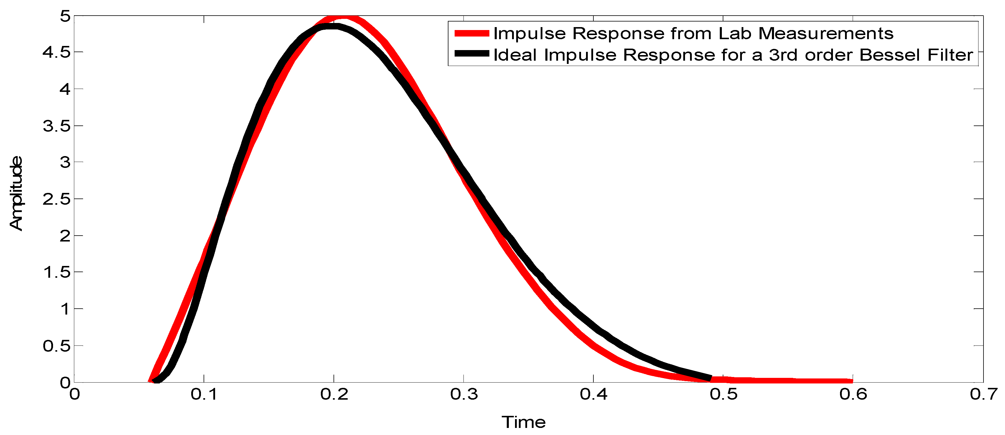
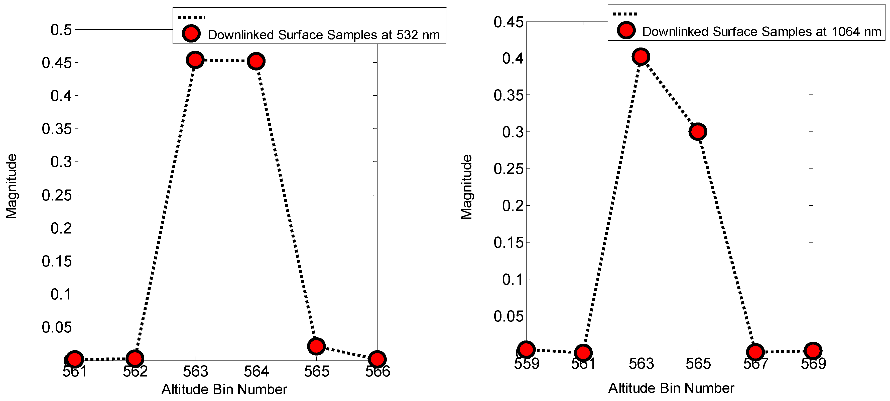
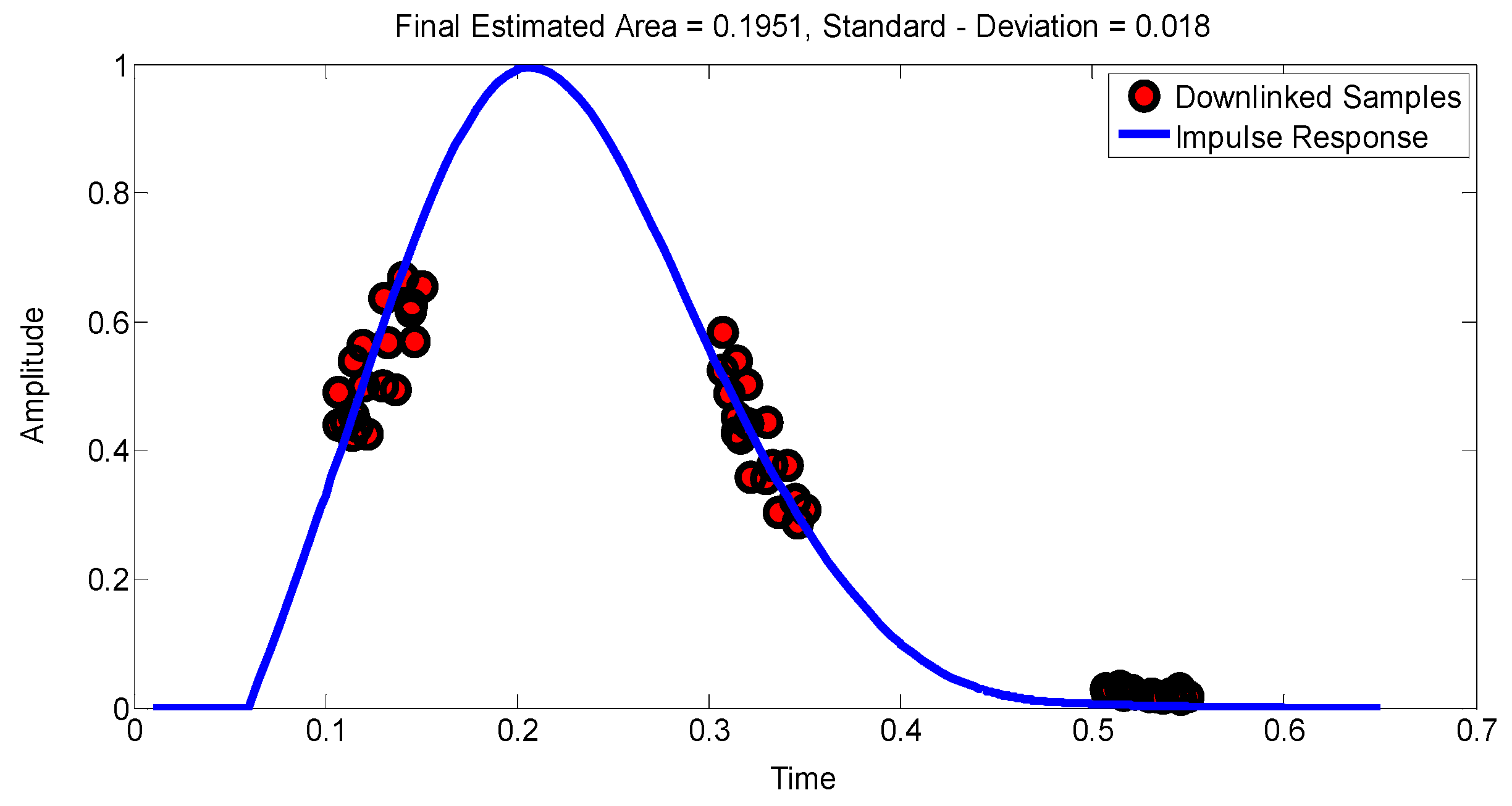
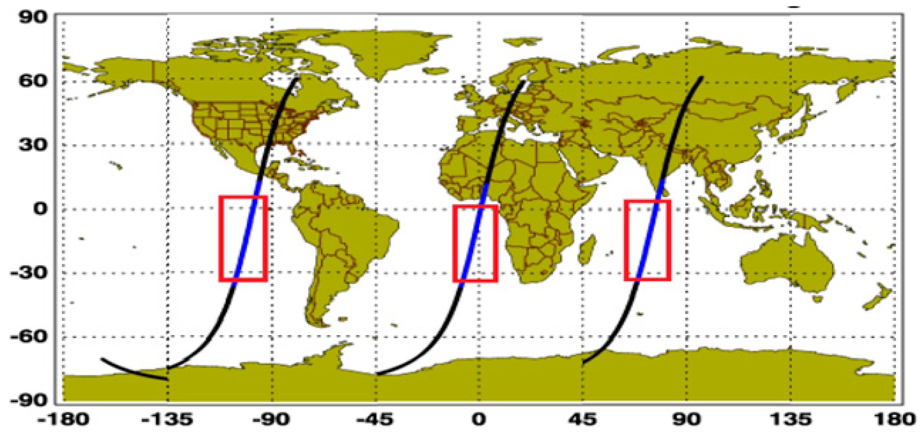
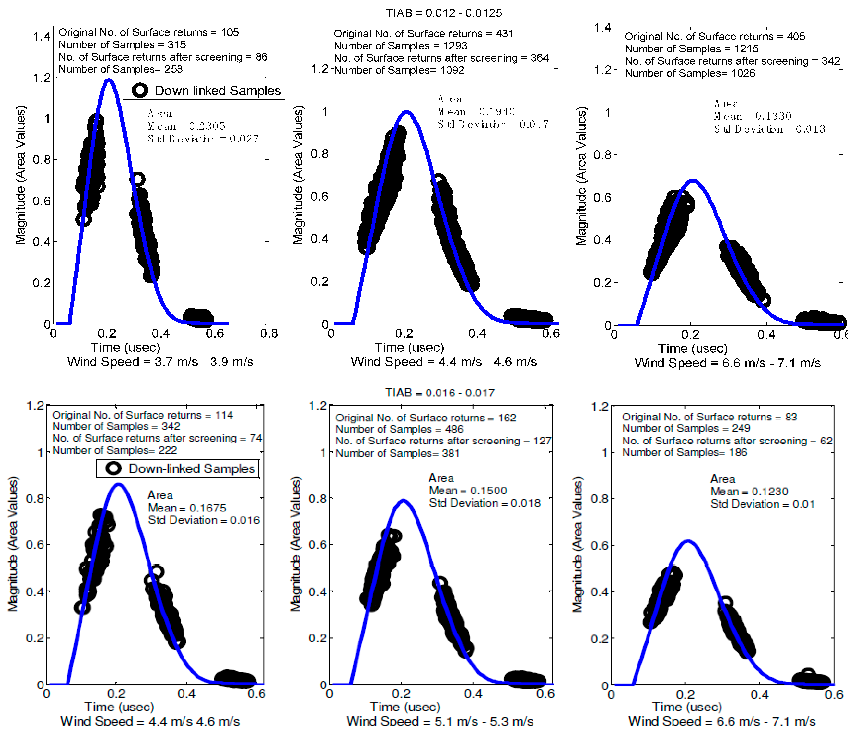
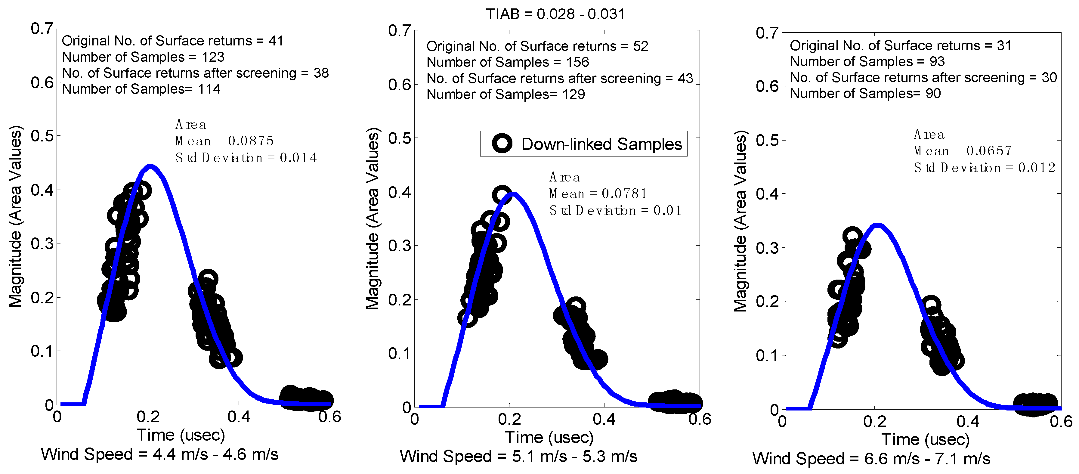
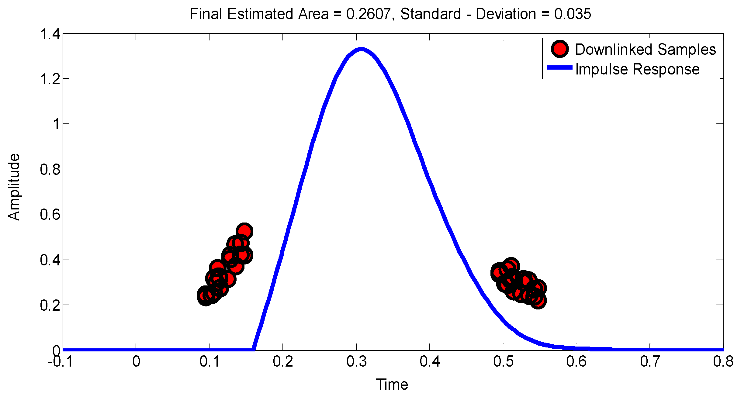
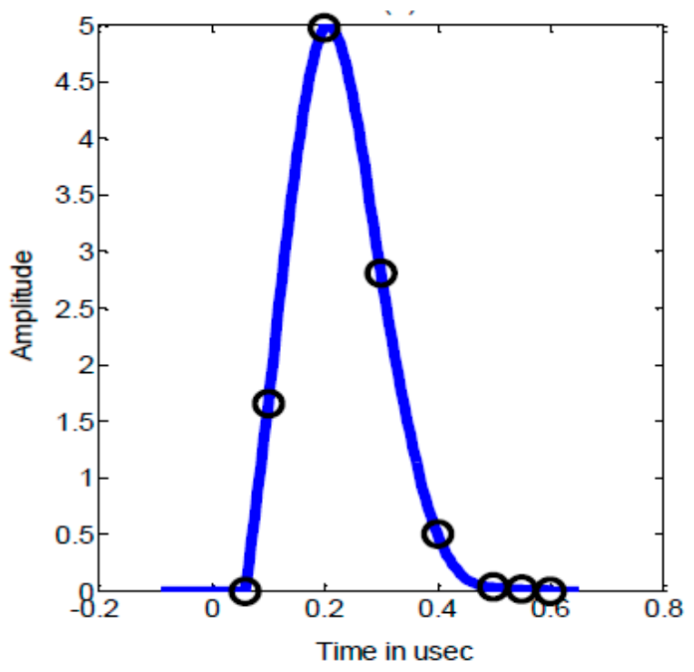
Example SR impulse response curve fits for data collected from the Southern Pacific Ocean region (see area defined in Figure 14) for the 532 nm channel are shown for several groupings in Figure 15. As described earlier in the previous section regarding Figure 12 and Figure 13, the response curve is the fit to the mean area determined from the average of the areas of all the retained down-linked samples in a group. For each grouping, the final estimated mean area and standard deviation, original number of surface returns/samples in the group and the number of surface returns/samples retained after data screening, are also provided. The areas and standard deviations for all the Southern Pacific Ocean 532 nm data groupings are given in

Table 1. Area under surface returns for various TIAB and surface wind speed values for Southern Pacific Ocean, 532 nm.

TIAB (sr−1)	Wind Speed	Wind Speed	Wind Speed	Wind Speed	Wind Speed
	3.7 m/s–3.9 m/s	4.4 m/s–4.6 m/s	5.1 m/s–5.3 m/s	5.5 m/s–6.0 m/s	6.6 m/s–7.1 m/s
0.012–0.0125	0.2305 ± 0.027	0.1940 ± 0.017	0.1625 ± 0.012	0.1538 ± 0.013	0.1330 ± 0.013
0.016–0.017	0.2041 ± 0.026	0.1675 ± 0.016	0.1500 ± 0.018	0.1358 ± 0.016	0.1230 ± 0.01
0.022–0.024	0.1474 ± 0.027	0.1128 ± 0.023	0.1094 ± 0.015	0.0960 ± 0.017	0.099 ± 0.017
0.028–0.031	0.1174 ± 0.019	0.0875 ± 0.014	0.0781 ± 0.010	0.0715 ± 0.012	0.0657 ± 0.012
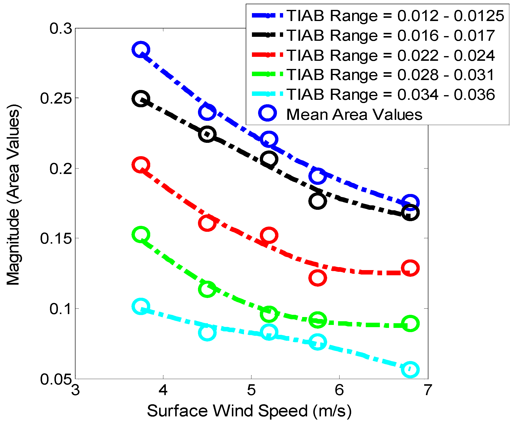
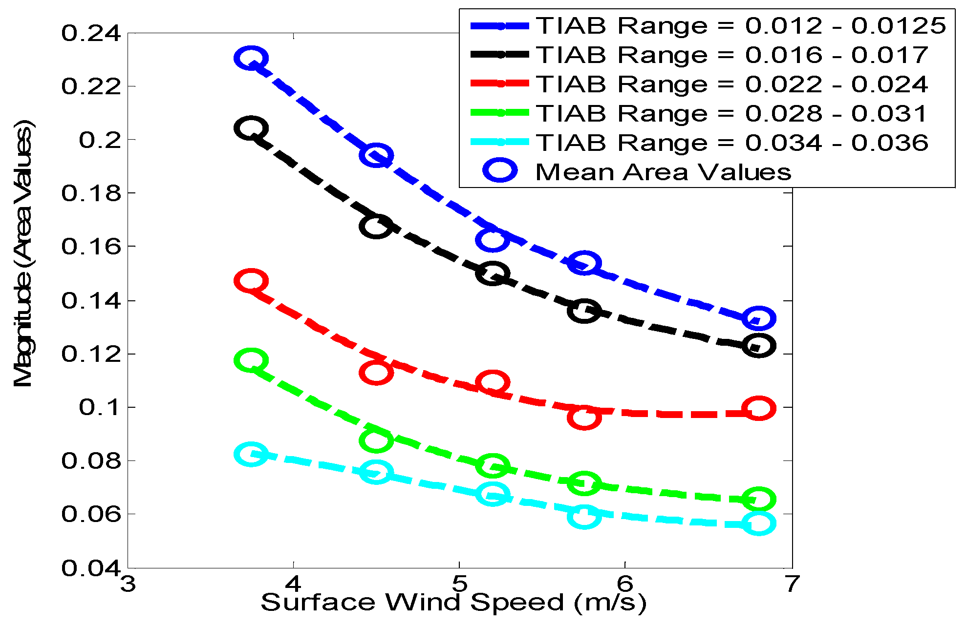
0.034–0.036	0.0824 ± 0.011	0.0759 ± 0.008	0.0674 ± 0.006	0.0589 ± 0.008	0.0565 ± 0.003

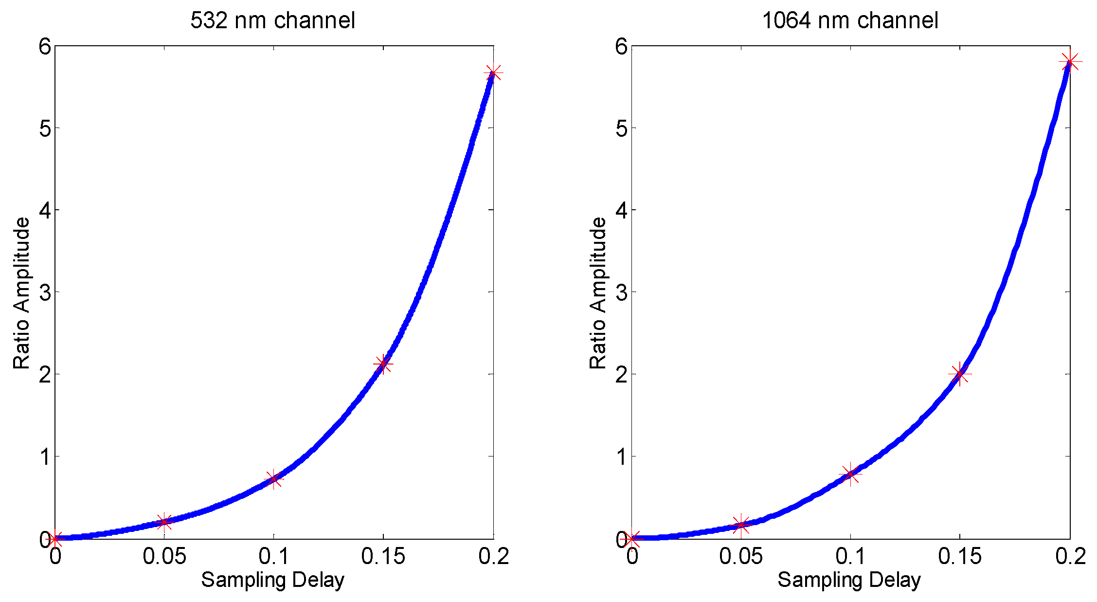
, and Figure 16 shows plots of these areas versus wind speed for each TIAB range. As expected, it can be seen from the figure that the areas progressively decrease with increasing TIAB. Corresponding results for the 1064 nm channel are given in

Table 2. Area under surface returns for various TIAB and surface wind speed values for Southern Pacific Ocean, 1064 nm.

TIAB (sr−1)	Wind Speed	Wind Speed	Wind Speed	Wind Speed	Wind Speed
	3.7 m/s–3.9 m/s	4.4 m/s–4.6 m/s	5.1 m/s–5.3 m/s	5.5 m/s–6.0 m/s	6.6 m/s–7.1 m/s
0.012–0.0125	0.2846 ± 0.026	0.2400 ± 0.023	0.2208 ± 0.018	0.1944 ± 0.013	0.1755 ± 0.019
0.016–0.017	0.2493 ± 0.04	0.2240 ± 0.02	0.2066 ± 0.018	0.1766 ± 0.028	0.1683 ± 0.018
0.022–0.024	0.2024 ± 0.037	0.1609 ± 0.03	0.1520 ± 0.032	0.1219 ± 0.026	0.129 ± 0.019
0.028–0.031	0.1525 ± 0.035	0.1135 ± 0.014	0.096 ± 0.003	0.0916 ± 0.016	0.0893 ± 0.012
0.034–0.036	0.1017 ± 0.003	0.0825 ± 0.006	0.0833 ± 0.011	0.0760 ± 0.004	0.0561 ± 0.01

and Figure 17. Similarly, the results for the Atlantic Ocean data analysis are given in

Table 3. Area under surface returns for various TIAB and surface wind speed values for Atlantic Ocean, 532 nm.

TIAB (sr−1)	Wind Speed	Wind Speed	Wind Speed	Wind Speed	Wind Speed
	3.7 m/s–3.9 m/s	4.4 m/s–4.6 m/s	5.1 m/s–5.3 m/s	5.5 m/s–6.0 m/s	6.6 m/s–7.1 m/s
0.012–0.0125	0.2250 ± 0.009	0.2037 ± 0.021	0.1865 ± 0.014	0.1342 ± 0.012	0.1283 ± 0.01
0.016–0.017	0.1951 ± 0.018	0.1780 ± 0.024	0.1585 ± 0.017	0.1227 ± 0.014	0.1181 ± 0.009
0.022–0.024	0.1380 ± 0.018	0.1097 ± 0.023	0.1085 ± 0.016	0.0895 ± 0.009	0.0870 ± 0.003
0.028–0.031	0.0945 ± 0.009	0.0854 ± 0.015	0.0810 ± 0.016	0.0683 ± 0.01	0.0607 ± 0.01
0.034–0.036	0.0727 ± 0.009	0.0637 ± 0.014	0.0600 ± 0.009	0.0540 ± 0.009	0.054 ± 0.008

and

Table 4. Area under surface returns for various TIAB and surface wind speed values for Atlantic Ocean, 1064 nm.

TIAB (sr−1)	Wind Speed	Wind Speed	Wind Speed	Wind Speed	Wind Speed
	3.7 m/s–3.9 m/s	4.4 m/s–4.6 m/s	5.1 m/s–5.3 m/s	5.5 m/s–6.0 m/s	6.6 m/s–7.1 m/s
0.012–0.0125	0.2861 ± 0.027	0.2537 ± 0.034	0.2387 ± 0.022	0.1820 ± 0.015	0.1608 ± 0.013
0.016–0.017	0.2607 ± 0.035	0.2374 ± 0.028	0.2008 ± 0.020	0.1649 ± 0.017	0.152 ± 0.023
0.022–0.024	0.1746 ± 0.03	0.1523 ± 0.028	0.1443 ± 0.028	0.1162 ± 0.01	0.1122 ± 0.007
0.028–0.031	0.1221 ± 0.022	0.1083 ± 0.013	0.0968 ± 0.008	0.0935 ± 0.004	0.0888 ± 0.016
0.034–0.036	0.1005 ± 0.01	0.0890 ± 0.018	0.0872 ± 0.011	0.0832 ± 0.008	0.0820 ± 0.01

, and the results for the Indian Ocean data analysis are given in

Table 5. Area under surface returns for various TIAB and surface wind speed values for Indian Ocean, 532 nm.

TIAB (sr−1)	Wind Speed	Wind Speed	Wind Speed	Wind Speed	Wind Speed
	3.7 m/s–3.9 m/s	4.4 m/s–4.6 m/s	5.1 m/s–5.3 m/s	5.5 m/s–6.0 m/s	6.6 m/s–7.1 m/s
0.012–0.0125	0.2315 ± 0.01	0.2092 ± 0.02	0.1791 ± 0.017	0.1538 ± 0.016	0.1262 ± 0.008
0.016–0.017	0.2048 ± 0.018	0.1801 ± 0.022	0.152 ± 0.018	0.14 ± 0.015	0.121 ± 0.007
0.022–0.024	0.1472 ± 0.026	0.1173 ± 0.021	0.1193 ± 0.008	0.1036 ± 0.021	0.0755 ± 0.011
0.028–0.031	0.0989 ± 0.01	0.0871 ± 0.017	0.0778 ± 0.014	0.0688 ± 0.01	0.0554 ± 0.005
0.034–0.036	0.0835 ± 0.009	0.0678 ± 0.008	0.0654 ± 0.008	0.0594 ± 0.008	0.0493 ± 0.005

and

Table 6. Area under surface returns for various TIAB and surface wind speed values for Indian Ocean, 1064 nm.

TIAB (sr−1)	Wind Speed	Wind Speed	Wind Speed	Wind Speed	Wind Speed
	3.7 m/s–3.9 m/s	4.4 m/s–4.6 m/s	5.1 m/s–5.3 m/s	5.5 m/s–6.0 m/s	6.6 m/s–7.1 m/s
0.012–0.0125	0.2704 ± 0.022	0.248 ± 0.034	0.2223 ± 0.018	0.2147 ± 0.026	0.158 ± 0.009
0.016–0.017	0.2436 ± 0.029	0.228 ± 0.018	0.1945 ± 0.022	0.1885 ± 0.026	0.152 ± 0.011
0.022–0.024	0.187 ± 0.032	0.1462 ± 0.032	0.1398 ± 0.017	0.132 ± 0.023	0.0938 ± 0.011
0.028–0.031	0.1273 ± 0.019	0.1133 ± 0.011	0.0963 ± 0.003	0.0973 ± 0.016	0.0813 ± 0.008
0.034–0.036	0.1134 ± 0.012	0.0928 ± 0.015	0.0878 ± 0.015	0.0813 ± 0.009	0.067 ± 0.005

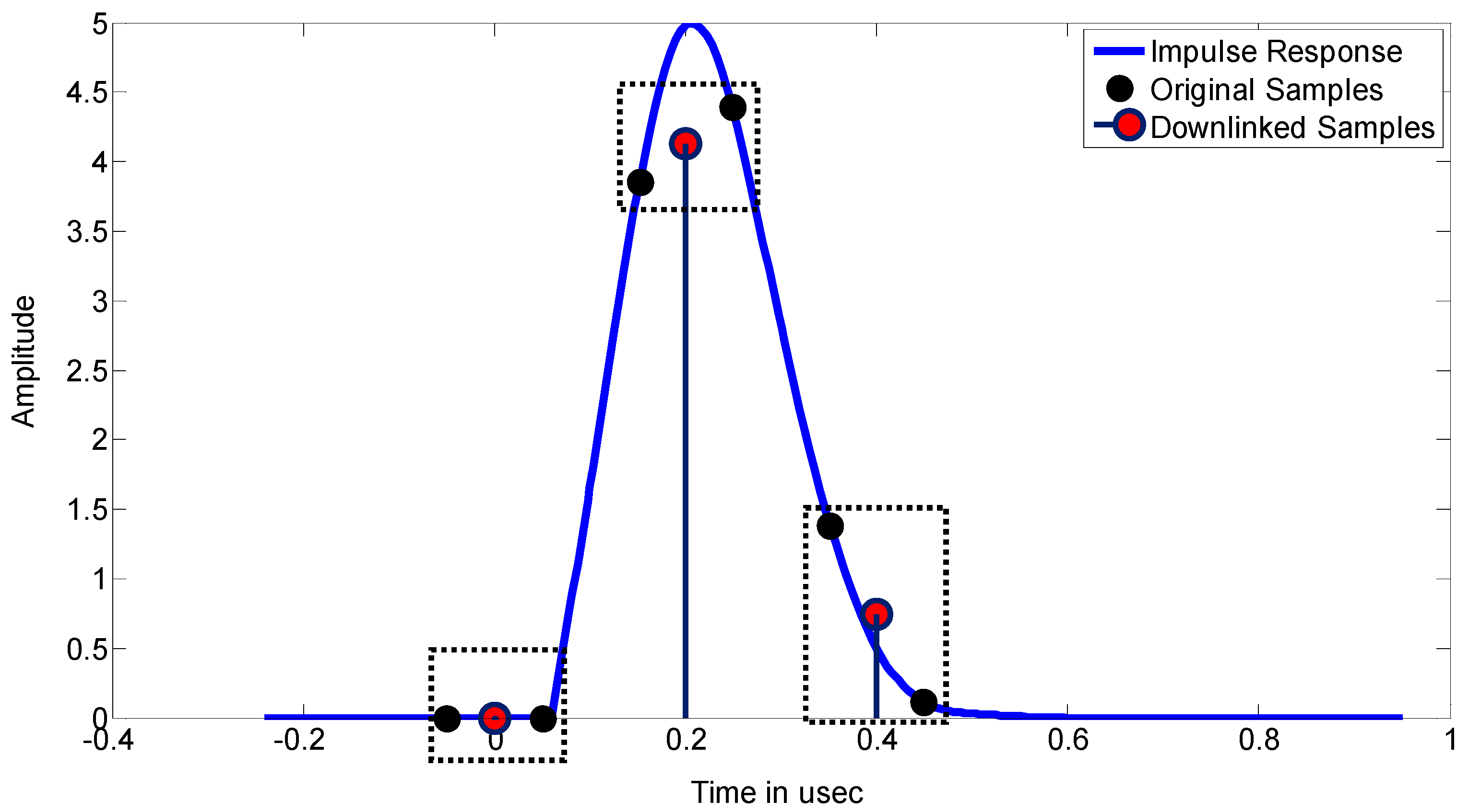
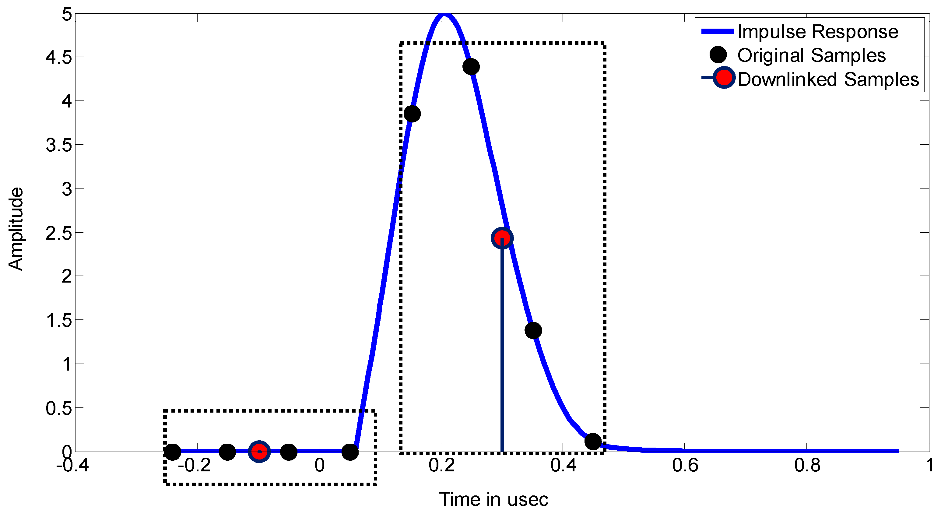
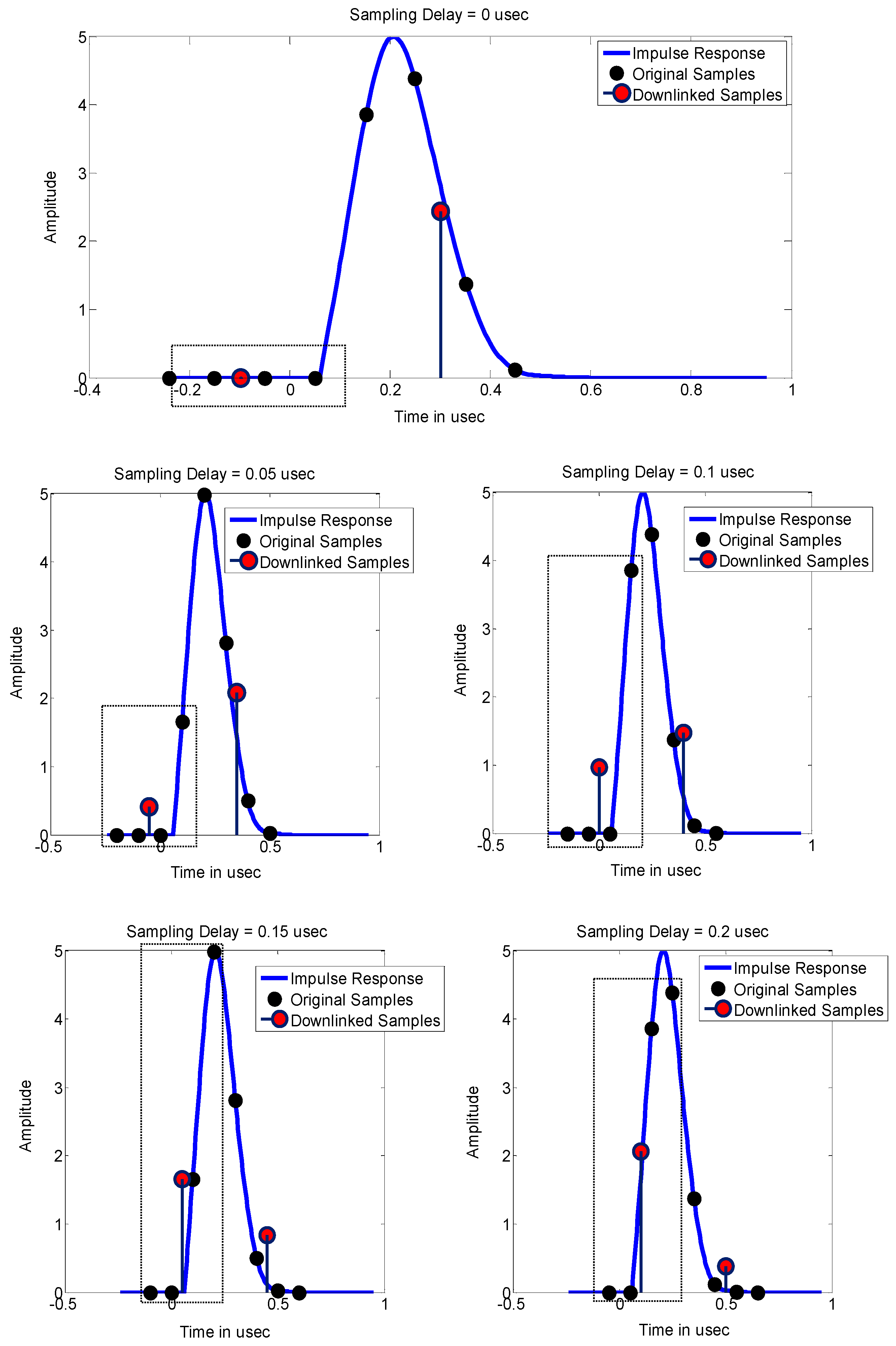
(the SR impulse response curve fits like those given in Figure 15 are not repeated for the Southern Pacific Ocean 1064 nm channel data or for the two channels for the other ocean regions as they all proved similar. Also, figures like Figure 16 and Figure 17 are not repeated for the other ocean regions as they also all proved similar). As can be seen in Figure 15 (and in the results obtained for curve fits for all ocean regions and both wavelengths) the greatest number of available down-linked samples/retained samples occurred at the lowest TIAB values (i.e., the lowest aerosol optical depth (AOD) values), indicating low AODs occurred most frequently.

From the several tables and figures, it can be seen that the data binning increments yielded tightly clustered areas for all groupings, the percent standard deviations for which ranged from a high of ~20% (one was as high as 23%) to a low of ~3%. For each channel/ocean region, the percent standard deviation of the areas was less than 12% for more than half the groupings (anywhere from 52% to 68%). The percentage of samples retained for the groupings was generally >~75%. The number of retained samples was >~100 for over 70% of the groupings, with only four groupings having <~50 samples (28 being the lowest). Thus, there were enough samples for good statistics in almost all cases. No trends of note were exhibited in the area standard deviations insofar as retained sample size, TIAB value and wind speed value. The estimated area statistics were found to be quite similar for both channels and all three ocean regions. Here it important to emphasize that the area standard deviations stem from a number contributions including (a) random signal noise; (b) temporal-spatial variability in signals assigned to a given finite size bin (recall that signals in a bin are not necessarily contiguous in space, time or stem from one aerosol type); (c) possible uncertainty in the wind speeds used to assign signals to a given bin; and (d) any error in calibration normalized out of the attenuated backscatter signals that were analyzed to obtain the areas. The fact noted above that the estimated area percent standard deviation was <12% for the majority of the groupings is relevant in that it implies the same fractional uncertainty (±0.12) for retrieving the aerosol round-trip transmittance, ${\mathrm{T}}_{\mathrm{a}}^2\left(\mathrm{z}\right)$, which in turn implies half that uncertainty for retrieving the Aerosol Optical Depth (AOD), or ±0.06; there will be more on this in a later sub-section. One would expect these uncertainties to be lower for a collection of contiguous/nearly contiguous shots from a localized spatial region with constant wind speed and fixed aerosol loading. To what extent such conditions may be met can be assessed by examining the statistics of areas retrieved for individual shots and running mean areas for various averaging intervals. Example retrievals along short orbit segments given later in the paper demonstrate that such averaging over fairly homogeneous aerosol regions indeed yields significantly lower uncertainties in the averaged AOD retrievals (although bias error may still be present).

3.3. Verification of Area Retrievals

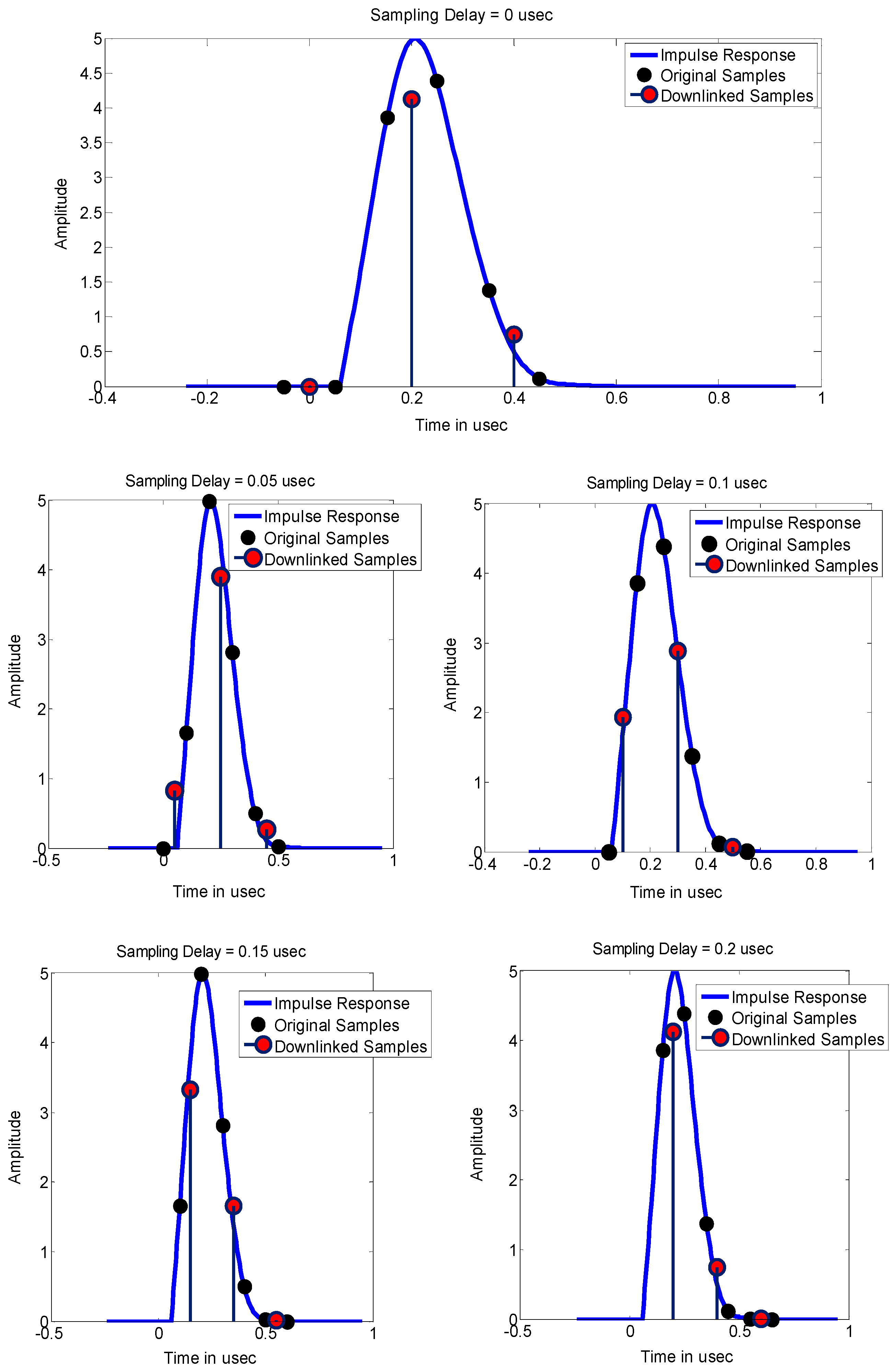
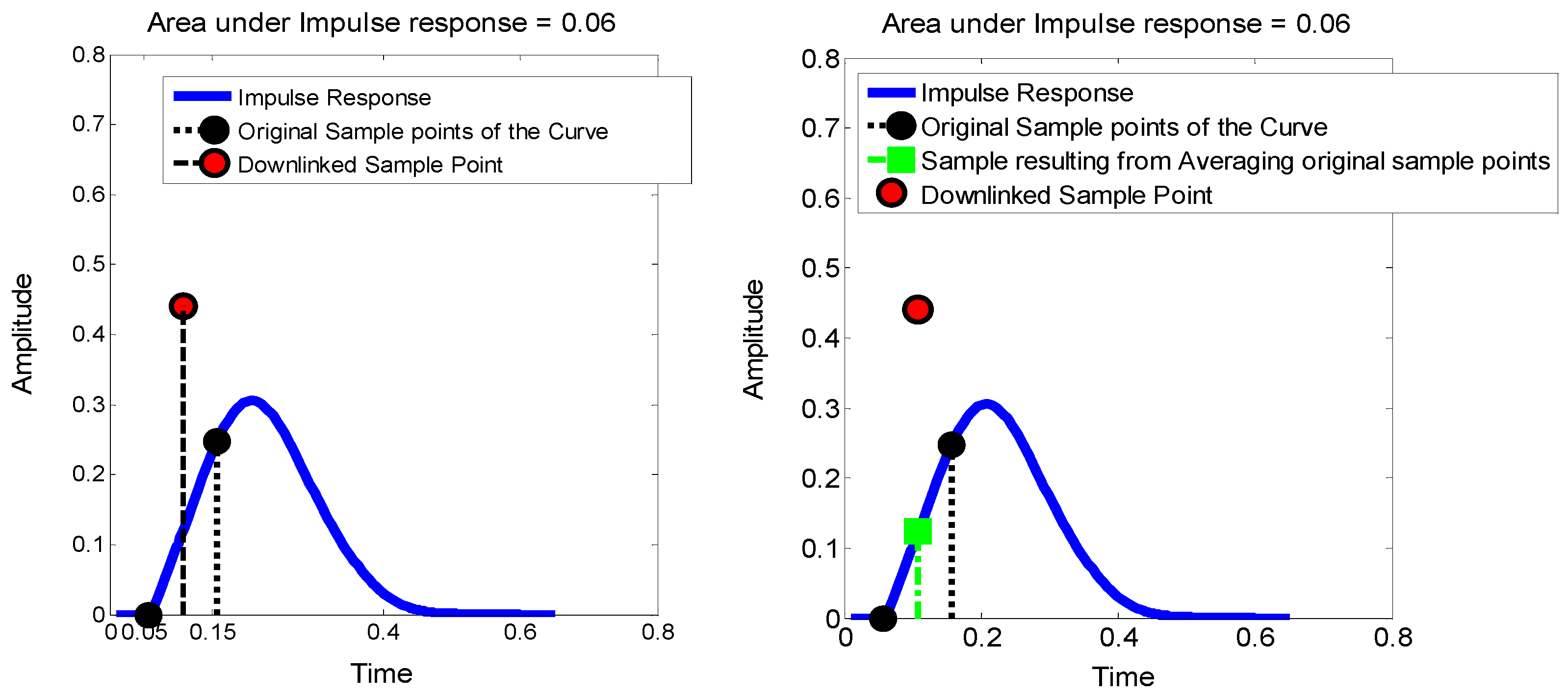
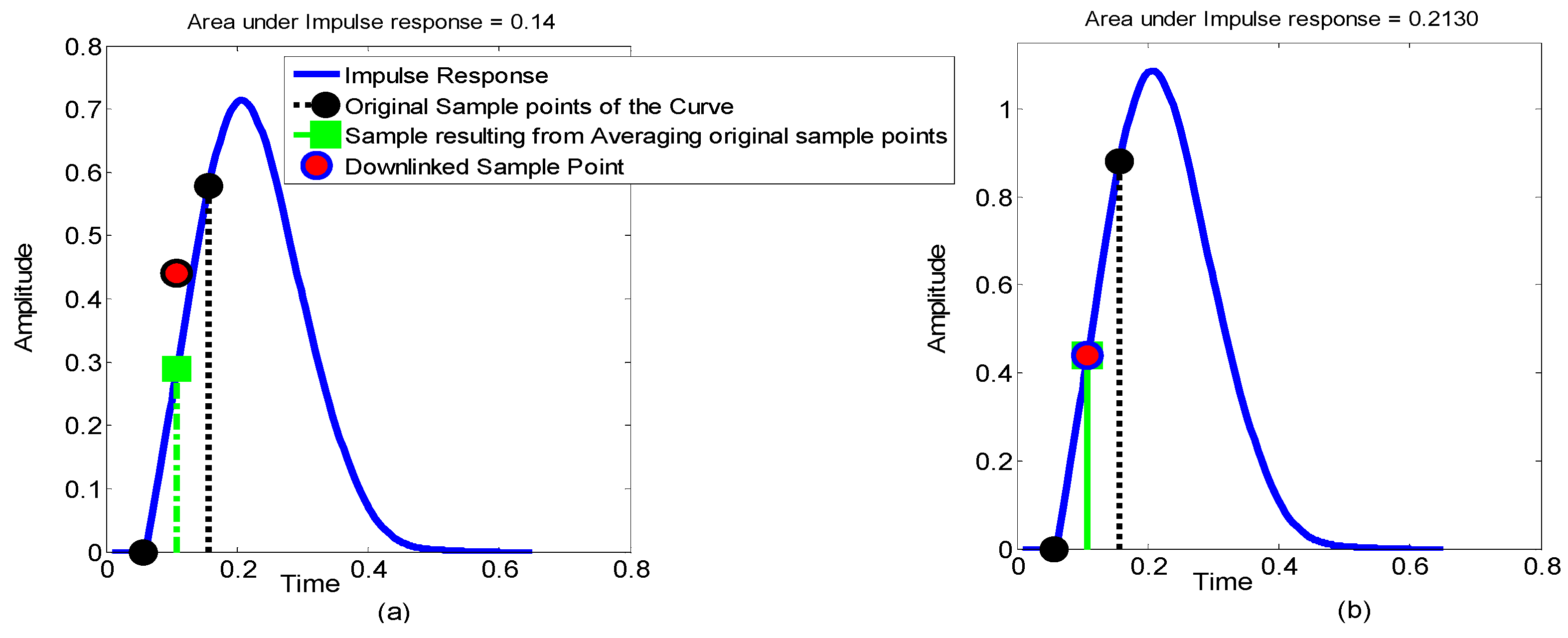
The SR area retrievals presented in the previous sub-section were estimated by a fitting procedure, described earlier in Section 2.5, wherein an assumed normalized impulse response curve was positioned and fitted to the down-linked SR samples for each shot, the curve fit determining the SR area for the shot. The individual estimated shot areas were grouped with areas for other shots with nearly the same TIAB and wind speed and, after screening for outliers, the retained group areas were averaged to obtain the estimated SR mean area for the group and associated standard deviation. Alternatively, SR areas may be predicted by the derived analytic relation for ${\mathrm{A}}_{\mathrm{LPF}}$ given in Equation (5), repeated here below with the round-trip transmission, ${\mathrm{T}}_{\mathsf{\lambda }}^2\left({\mathrm{z}}_{\mathrm{s}}\right)$, resolved into the aerosol, Rayleigh and ozone components as was done in Equation (10).

$${\mathrm{A}}_{\mathrm{LPF}}=\frac{2{\mathrm{T}}_{\mathsf{\lambda }}^2\left(\mathrm{z}\right){\mathrm{R}}_{\mathsf{\lambda }}}{\mathrm{c}}=\frac{2{\mathrm{T}}_{\mathrm{a}}^2\left(\mathrm{z}\right){\mathrm{T}}_{\mathrm{R}}^2\left(\mathrm{z}\right){\mathrm{T}}_{\mathrm{Ozone}}^2\left(\mathrm{z}\right){\mathrm{R}}_{\mathsf{\lambda }}}{\mathrm{c}}$$

(13)

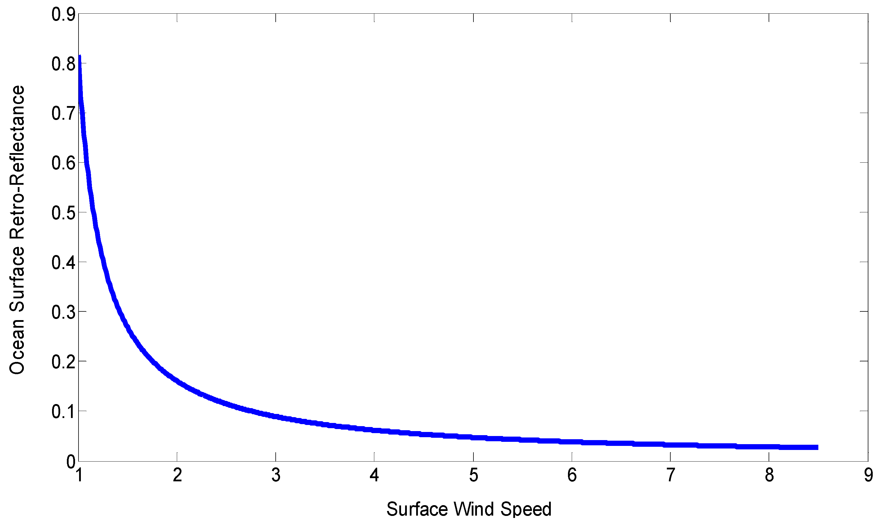
To predict ${\mathrm{A}}_{\mathrm{LPF}}$ from this analytic relation requires specification of ${\mathrm{R}}_{\mathsf{\lambda }}$, which can be computed from the wind speed model and the wind speed data for a given shot in the CALIPSO data base, as well as ${\mathrm{T}}_{\mathsf{\lambda }}^2\left({\mathrm{z}}_{\mathrm{s}}\right)$. The Rayleigh and ozone round-trip transmissions are fairly constant over oceans and can be computed from the information in the CALIPSO data base, the product of which for 532 nm is to a very close approximation ${\mathrm{T}}_{\mathrm{R}}^2\left({\mathrm{z}}_{\mathrm{s}}\right)\times {\mathrm{T}}_{\mathrm{Ozone}}^2\left({\mathrm{z}}_{\mathrm{s}}\right)$ = 0.798 × 0.96 = 0.76. The Rayleigh and ozone attenuations for 1064 nm are quite small so that ${\mathrm{T}}_{\mathrm{R}}^2\left({\mathrm{z}}_{\mathrm{s}}\right)\times {\mathrm{T}}_{\mathrm{Ozone}}^2\left({\mathrm{z}}_{\mathrm{s}}\right)$ = ~1 is a reasonable approximation. ${\mathrm{T}}_{\mathrm{a}}^2\left({\mathrm{z}}_{\mathrm{s}}\right)$ is generally unknown, but by selecting data for the aerosol free, clean atmospheres (for 532 nm TIAB < 0.0125), it can be approximated as unity. Thus, for data with TIAB < 0.0125, ${\mathrm{A}}_{\mathrm{LPF}}$ may be approximated for 532 nm as

$${\mathrm{A}}_{\mathrm{LPF}}=\frac{2{\mathrm{T}}^2{\mathrm{R}}_{532}}{\mathrm{c}}=\frac{2{\mathrm{T}}_{\mathrm{a}}^2\times {\mathrm{T}}_{\mathrm{R}}^2\times {\mathrm{T}}_{\mathrm{Ozone}}^2\times {\mathrm{R}}_{532}}{\mathrm{c}}=\frac{2\times 1\times 0.76\times {\mathrm{R}}_{532}}{\mathrm{c}}$$

(14)

and for 1064 nm as

$${\mathrm{A}}_{\mathrm{LPF}}=\frac{2{\mathrm{T}}^2{\mathrm{R}}_{1064}}{\mathrm{c}}=\frac{2\times {\mathrm{T}}_{\mathrm{a}}^2\times {\mathrm{T}}_{\mathrm{R}}^2\times {\mathrm{R}}_{1064}}{\mathrm{c}}=\frac{2\times 1\times 1\times {\mathrm{R}}_{1064}}{\mathrm{c}}$$

(15)

Computing analytically predicted areas (APA) by these relations for the various wind speed bins defined earlier (mean wind of each wind speed bin used to calculate ${\mathrm{R}}_{\mathsf{\lambda }}$) and using the data-estimated areas (DEA) presented earlier (e.g., Table 1) for these wind speed bins and TIAB < 0.0125, a comparison may be made of the two sets of area determinations as shown in

Table 7. Comparing analytically predicted and data-estimated areas under surface returns for the Southern Pacific oceanic region for clean atmospheric conditions.

Wind Speed	Analytically Predicted Surface Return area APA at 532 nm	Data-Estimated Area DEA at 532 nm	Ratio DEA/APA for 532 nm	Analytically Predicted Surface Return Area APA at 1064 nm	Data-Estimated Area DEA at 1064 nm	Ratio DEA/APA for 1064 nm
3.7 m/s–3.9 m/s	0.2334	0.2305 ± 0.027	0.9875	0.2891	0.2846 ± 0.026	0.9844
4.4 m/s–4.6 m/s	0.1979	0.1940 ± 0.017	0.9802	0.2452	0.2400 ± 0.023	0.9787
5.1 m/s–5.3 m/s	0.1747	0.1625 ± 0.012	0.9301	0.2164	0.2208 ± 0.018	1.0203
5.5 m/s–6.0 m/s	0.1612	0.1538 ± 0.013	0.9539	0.1998	0.1944 ± 0.013	0.9729
6.6 m/s–7.1 m/s	0.1380	0.1330 ± 0.013	0.9640	0.1710	0.1755 ± 0.019	1.026

for the Southern Pacific Ocean data collection.

It can be seen that the ratios of DEA/APA are close to one and well within the DEA standard deviations. Similar results were found for the Atlantic and Indian Ocean ratios as shown in

Table 8. Ratios of analytically predicted and data-estimated areas under surface returns for the Atlantic and Indian Ocean regions for clean atmospheric conditions.

Wind Speed	Ratio DEA/APA for 532 nm	Ratio DEA/APA for 1064 nm	Ratio DEA/APA for 532 nm	Ratio DEA/APA for 1064 nm
	(Atlantic Ocean)	(Atlantic Ocean)	(Indian Ocean)	(Indian Ocean)
3.7 m/s–3.9 m/s	0.9640	0.9896	0.9918	0.9353
4.4 m/s–4.6 m/s	1.0292	1.0346	1.0570	1.0114
5.1 m/s–5.3 m/s	1.0675	1.1030	1.0251	1.0272
5.5 m/s–6.0 m/s	0.8323	0.9109	0.9539	1.0745
6.6 m/s–7.1 m/s	0.9299	0.9403	0.9147	0.9240

(The DEA bin values are not repeated, but can be found in Table 3, Table 4, Table 5 and Table 6 nor are the APA bin values as they are same for all oceans). Averaging the ratios over all wind speeds yields the results shown in

Table 9. Mean and standard deviation of DEA/APA ratios calculated over all wind speeds for each oceanic region at 532 nm wavelength for clean atmospheric conditions.

Region	Mean Ratio (Overall Wind Speeds)	Standard Deviation
Southern Pacific	0.9631	0.0227
Atlantic	0.9646	0.0915
Indian	0.9885	0.0563

and

Table 10. Mean and standard deviation of DEA/APA ratios calculated over all wind speeds for each oceanic region at 1064 nm wavelength for clean atmospheric conditions.

Region	Mean Ratio (Overall Wind Speeds)	Standard Deviation
Southern Pacific	0.9965	0.0017
Atlantic	0.9957	0.0763
Indian	0.9945	0.0637

.

It can be seen for the 1064 nm channel that the ratios for all oceans are within 1% of unity, while the results for the 532 nm channel fall within 4% of unity, indicating perhaps a slight bias off-set to lower DEA values, although the ratios are generally within their standard deviations. Such a bias could arise due to some aerosol contamination in the 532 nm signals assumed to be aerosol free for TIAB < 0.0125, or if the impulse response assumed for the 532 nm channel was slightly different than the actual impulse response for that channel, or possible error either in the lidar calibration or the reflectance model/wind speed input to the model. No such bias is suggested for the 1064 nm channel, indicating an absence of any significant effect from lidar calibration error or the reflectance model/wind speed input to the model having caused a bias (which would also affect the 532 nm results, thereby seemingly removing these errors as the source of the 532 nm off-set). Hence, the slight deviations from unity for either wavelength, being within there standard deviations, may just stem from normally expected variability. All in all, the agreement between the data estimated and analytically predicted areas is excellent, indicating corroboration of the technique and results presented earlier for estimating the area of SR signals from the down-linked SR samples.

3.4. Aerosol Retrievals

Rearranging Equation (13), ${\mathrm{T}}_{\mathrm{a}}^2\left({\mathrm{z}}_{\mathrm{s}}\right)$ is given by

$${\mathrm{T}}_{\mathrm{a}}^2\left({\mathrm{z}}_{\mathrm{s}}\right)=\frac{{\mathrm{cA}}_{\mathrm{LPF}}}{2{\mathrm{R}}_{\mathsf{\lambda }}{\mathrm{T}}_{\mathrm{R}}^2\left({\mathrm{z}}_{\mathrm{s}}\right){\mathrm{T}}_{\mathrm{Ozone}}^2\left({\mathrm{z}}_{\mathrm{s}}\right)}$$

(16)

Using the approximations given earlier for ${\mathrm{T}}_{\mathrm{R}}^2\left({\mathrm{z}}_{\mathrm{s}}\right)\times {\mathrm{T}}_{\mathrm{Ozone}}^2\left({\mathrm{z}}_{\mathrm{s}}\right)$, Equation (16) reduces, for both wavelengths, to

$${\mathrm{T}}_{\mathrm{a}}^2\left({\mathrm{z}}_{\mathrm{s}}\right)=\frac{{\mathrm{cA}}_{\mathrm{LPF}}}{2\times {\mathrm{R}}_{532}\times 0.76}$$

(17)

$${\mathrm{T}}_{\mathrm{a}}^2\left({\mathrm{z}}_{\mathrm{s}}\right)=\frac{{\mathrm{cA}}_{\mathrm{LPF}}}{2\times {\mathrm{R}}_{1064}}$$

(18)

In turn, the aerosol optical depth (AOD), τ_a, is given by

$${\mathsf{\tau }}_{\mathrm{a}}=-\frac{{\log }_{\mathrm{e}}\left({\mathrm{T}}_{\mathrm{a}}^2\left({\mathrm{z}}_{\mathrm{s}}\right)\right)}{2}$$

(19)

By differential analysis, the fractional uncertainty in ${\mathrm{T}}_{\mathrm{a}}^2$ due to uncertainty in ${\mathrm{A}}_{\mathrm{LPF}}$ is

$$\frac{{\mathrm{\Delta }\mathrm{T}}_{\mathrm{a}}^2}{{\mathrm{T}}_{\mathrm{a}}^2}=\frac{{\mathrm{\Delta }\mathrm{A}}_{\mathrm{LPF}}}{{\mathrm{A}}_{\mathrm{LPF}}}$$

(20)

and the corresponding uncertainty in AOD is half that,

$${\mathrm{\Delta }\mathsf{\tau }}_{\mathrm{a}}=-0.5\times \frac{{\mathrm{\Delta }\mathrm{A}}_{\mathrm{LPF}}}{{\mathrm{A}}_{\mathrm{LPF}}}$$

(21)

Example retrievals of ${\mathrm{T}}_{\mathrm{a}}^2$ and AOD by Equations (16) and (19) applied to the ${\mathrm{A}}_{\mathrm{LPF}}$ retrievals given earlier (Table 1, Table 2, Table 3, Table 4, Table 5 and Table 6), for one wind speed bin (5.1–5.3 m/s) and two TIAB bins (0.016–0.017 and 0.028–0.031), for all three ocean regions, are given in

Table 11. Representative example retrievals of aerosol round-trip transmission and AOD for Southern Pacific Ocean region.

TIAB (sr−1)	Ta2	AOD	Ta2	AOD	Ta2	AOD	Ta2	AOD
	(532 nm, High/Low Method)	(532 nm, High/Low Method)	(532 nm, Analytic Method)	(532 nm, Analytic Method)	(1064 nm, High/Low Method)	(1064 nm, High/Low Method)	(1064 nm, Analytic Method)	(1064 nm, Analytic Method)
0.016–0.017	0.9281 ± 0.131	0.037 ± 0.07	0.8558 ± 0.103	0.078 ± 0.0601	0.9357 ± 0.112	0.033 ± 0.059	0.9654 ± 0.084	0.018 ± 0.043
0.028–0.031	0.4832 ± 0.071	0.364 ± 0.073	0.4456 ± 0.057	0.404 ± 0.0639	0.4348 ± 0.038	0.416 ± 0.043	0.4486 ± 0.014	0.401 ± 0.015

,

Table 12. Representative example retrievals of aerosol round-trip transmission and AOD for Atlantic Ocean region.

TIAB (sr−1)	Ta2	AOD	Ta2	AOD	Ta2	AOD	Ta2	AOD
	(532 nm, High Low Method)	(532 nm, High Low Method	(532 nm, Analytic Method)	(532 nm, Analytic Method)	(1064 nm, High Low Method)	(1064 nm, High Low Method	(1064 nm, Analytic Method)	(1064 nm, Analytic Method)
0.016–0.017	0.8500 ± 0.111	0.081 ± 0.065	0.9043 ± 0.097	0.050 ± 0.053	0.8412 ± 0.114	0.086 ± 0.067	0.9383 ± 0.086	0.032 ± 0.045
0.028–0.031	0.4343 ± 0.092	0.417 ± 0.105	0.4621 ± 0.091	0.386 ± 0.098	0.4055 ± 0.053	0.451 ± 0.065	0.4523 ± 0.042	0.397 ± 0.046

and

Table 13. Representative example retrievals of aerosol round-trip transmission and AOD for Indian Ocean region.

TIAB (sr−1)	Ta2	AOD	Ta2	AOD	Ta2	AOD	Ta2	AOD
	(532 nm, High Low Method)	(532 nm, High Low Method	(532 nm, Analytic Method)	(532 nm, Analytic Method)	(1064 nm, High Low Method)	(1064 nm, High Low Method	(1064 nm, Analytic Method)	(1064 nm, Analytic Method)
0.016–0.017	0.8487 ± 0.129	0.082 ± 0.075	0.8672 ± 0.102	0.071 ± 0.058	0.8749 ± 0.122	0.067 ± 0.064	0.9089 ± 0.103	0.048 ± 0.056
0.028–0.031	0.4344 ± 0.088	0.417 ± 0.101	0.4439 ± 0.080	0.406 ± 0.090	0.4332 ± 0.038	0.418 ± 0.043	0.4500 ± 0.014	0.399 ± 0.015

. Also given in the tables are retrievals by an alternate method, called the High/Low method.

As the ratio of ${\mathrm{A}}_{\mathrm{LPF}}$ for two different TIAB values and the same wind speed equals the corresponding ratio of ${\mathrm{T}}_{\mathrm{a}}^2$, the aerosol round-trip transmission for a high TIAB, ${\mathrm{T}}_{\mathrm{a}}^2$ (high TIAB), is given by

$${\mathrm{T}}_{\mathrm{a}}^2\left(\mathrm{High}\mathrm{TIAB}\right)=\frac{{\mathrm{A}}_{\mathrm{LPF}}\left(\mathrm{High}\mathrm{TIAB}\right)}{{\mathrm{A}}_{\mathrm{LPF}}\left(\mathrm{Low}\mathrm{TIAB}\right)}\times {\mathrm{T}}_{\mathrm{a}}^2\left(\mathrm{Low}\mathrm{TIAB}\right)$$

(22)

Selecting the low TIAB to be for the clean, aerosol-free atmosphere case (TIAB < 0.0125) for which the aerosol round-trip transmission is approximated as unity, ${\mathrm{T}}_{\mathrm{a}}^2\left(\mathrm{High}\mathrm{TIAB}\right)$ simply equals the ratio ${\mathrm{A}}_{\mathrm{LPF}}\left(\mathrm{High}\mathrm{TIAB}\right)/{\mathrm{A}}_{\mathrm{LPF}}\left(\mathrm{Clean}\mathrm{Atmosphere}\right)$. An advantage of the High/Low method is that it eliminates the need for an accurate surface reflectance-wind speed model as the reflectance cancels in the area ratio, although the standard deviation for the retrieved aerosol round-trip transmission is generally a little higher than for the analytic method because the standard deviation of each of the areas in the ratio must be taken into account. It can be seen from the tables that the ${\mathrm{T}}_{\mathrm{a}}^2$ retrievals for both methods agree well within their respective standard deviations (most within ~0.05) and the AODs agree within ~0.05 (most within ~0.03). This, as with the results in Table 9 and Table 10, again suggests that errors in either the reflectance model/wind speed inputs to the model for determining the analytically determined AODs or lidar calibration error (which could affect the High/Low determinations) were not significant. The results for the other wind speed and TIAB bins are similar insofar as having about the same variability/uncertainty in retrieved ${\mathrm{T}}_{\mathrm{a}}^2$ and AOD. The AOD uncertainty is comparable to the AOD retrievals for the lower TIAB (0.016 to 0.017), making it difficult to quantitatively interpret these AOD, but the higher TIAB (0.028 to 0.031) AODs generally appear good enough to be quantitatively useful. Examination of the AOD spectral ratio (532/1064) revealed that this ratio ranged from about 1.05 to 1.2, most being 1.1 or greater, which is within the range of the ratios for dust and marine aerosol models (e.g., [15]). The CALIPSO browse images for the ~15 days and regions for the observations investigated here revealed that the aerosols were mainly identified as marine aerosols.

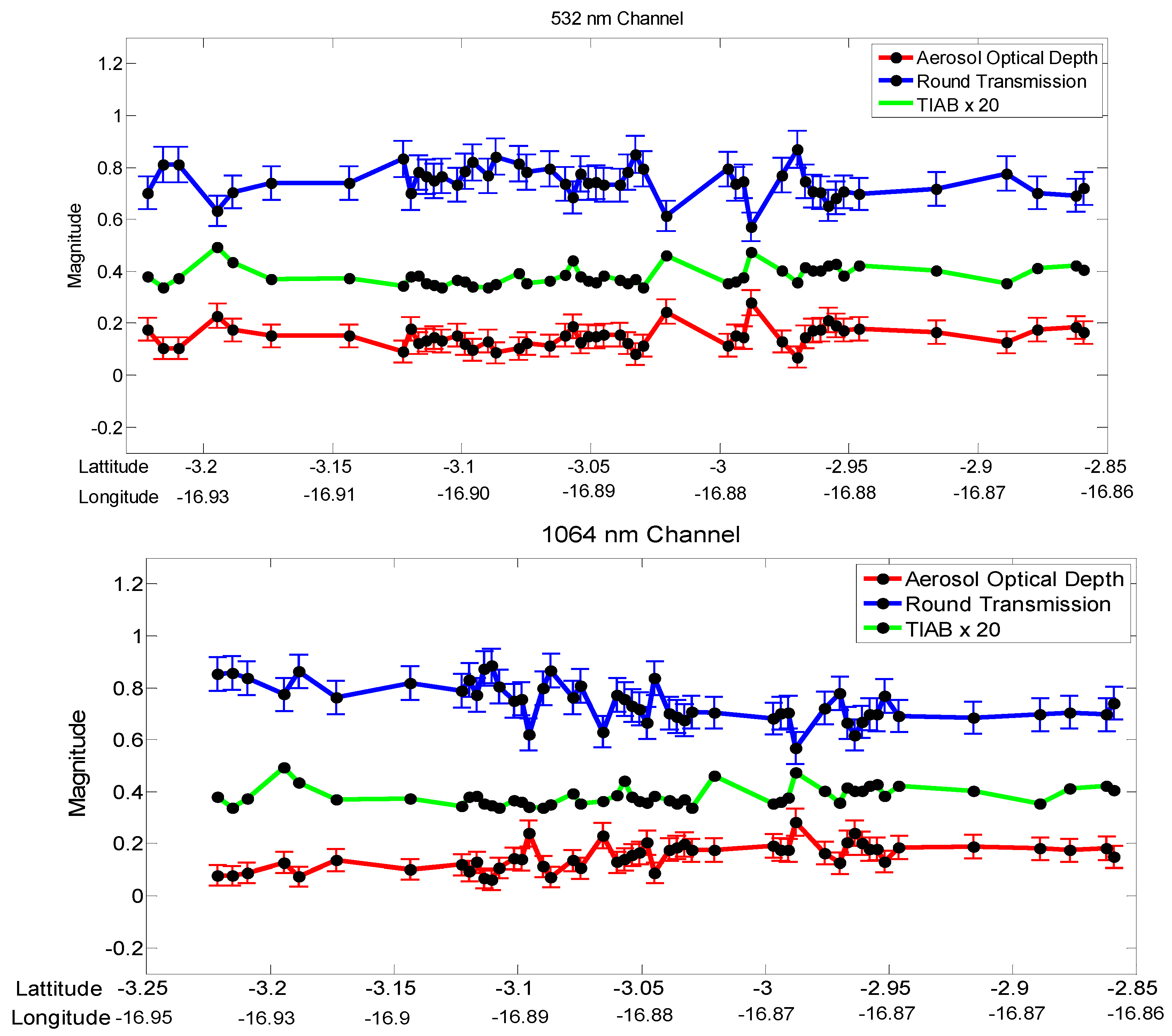
Equations (16) and (19) were used to retrieve the AOD for a sample collection of ~50 nearly contiguous lidar shots for an orbit segment over the Atlantic Ocean. These shots were for a 9 May 2011 segment between the lat-lon positions (−3.3 lat, −16.96 lon) and (−2.85 lat, −16.86 lon), which corresponds to about ~75 shots, amongst which ~50 had detectable surface returns (with 0.0125 < TIAB < 0.035). Figure 18 shows the per-shot retrievals of ${\mathrm{T}}_{\mathrm{a}}^2$ and AOD for both wavelengths, and the TIAB times 20 (to be on scale) is also shown. The correlation of TIAB with AOD and anti-correlation with ${\mathrm{T}}_{\mathrm{a}}^2$ is clearly evident. The mean AODs are about the same for both wavelengths (0.155 for 532 nm and 0.148 for 1064 nm, each with a standard deviation uncertainty of ±0.045). The AOD is fairly flat over the segment for 532 nm, but displays a slight rising trend for 1064 nm. As such, averaging over several shots should reduce the per-shot AOD uncertainty (~±0.05); averaging over six consecutive shots (2 km averaging) reduced the AOD uncertainty to <±0.02 for the averaged AODs. The spectral ratio (1064/532) of ${\mathrm{T}}_{\mathrm{a}}^2$ has a mean of ~1.01, ranging from ~0.96 to ~1.12, while for AOD the mean spectral ratio is ~1.04, ranging from ~0.70 to ~1.15 (rather variable). Clearly, the mean spectral ratios are fairly neutral, and the mean AOD ratio is close to the range that applies to dust and marine aerosols (e.g., [15]). Examining the CALIPSO browse image for this segment revealed that the aerosols present were indeed mainly identified as marine aerosols.

The spectral ratio of aerosol round-trip transmission is of further interest because it can be estimated directly from the spectral ratio of the ${\mathrm{A}}_{\mathrm{LPF}}$ without having to assume a particular wind speed model, save accounting for the difference in Fresnel reflectance due to the ocean refractive index difference at the two wavelengths. From Equation (13), the spectral ratio (1064/532) of ${\mathrm{A}}_{\mathrm{LPF}}$, using the numerical estimates for the round-trip Rayleigh and ozone transmittances given earlier, reduces to

$$\frac{{\mathrm{A}}_{\mathrm{LPF}1064}}{{\mathrm{A}}_{\mathrm{LPF}532}}=\frac{1}{0.76}\times \frac{{\mathrm{R}}_{1064}}{{\mathrm{R}}_{532}}\times \frac{{\mathrm{T}}_{\mathrm{a}1064}^2}{{\mathrm{T}}_{\mathrm{a}532}^2}$$

(23)

Assuming the reflectances are equal at each wavelength, except for the refractive index difference in the Fresnel reflectances, having a spectral ratio of ~1/1.06 (for 1064 to 532), Equation (23) reduces to

$$\frac{{\mathrm{A}}_{\mathrm{LPF}1064}}{{\mathrm{A}}_{\mathrm{LPF}532}}=\frac{1}{0.76}\times \frac{{\mathrm{R}}_{1064}}{{\mathrm{R}}_{532}}\times \frac{{\mathrm{T}}_{\mathrm{a}1064}^2}{{\mathrm{T}}_{\mathrm{a}532}^2}=\frac{1}{0.76}\times \frac{1}{1.06}\times \frac{{\mathrm{T}}_{\mathrm{a}1064}^2}{{\mathrm{T}}_{\mathrm{a}532}^2}=1.241\times \frac{{\mathrm{T}}_{\mathrm{a}1064}^2}{{\mathrm{T}}_{\mathrm{a}532}^2}$$

(24)

For the clean, aerosol-free situation (TIAB < 0.0125), the aerosol transmission spectral ratio reduces to unity and the ${\mathrm{A}}_{\mathrm{LPF}}$ spectral ratio is simply 1.241. Examining the ${\mathrm{A}}_{\mathrm{LPF}}$ values for 1064 nm and 532 nm given earlier in Table 1, Table 2, Table 3, Table 4, Table 5 and Table 6, for TIAB < 0.0125 and averaging overall wind speeds per ocean region, yields mean area spectral ratios, ${\mathrm{A}}_{\mathrm{LPF}1064}/{\mathrm{A}}_{\mathrm{LPF}532}$, of 1.283, 1.281 and 1.248 for the Southern Pacific Ocean, Atlantic Ocean and Indian Ocean, respectively, all within ~3% of the 1.241 value, substantiating the validity of the analytic relation given in Equation (24). This ~3% difference, as with the ~4% difference noted regarding the 532 nm results in Table 7, could arise due to some aerosol contamination or the assumed impulse response curve for the 532 nm channel being slightly different than the actual impulse response for that channel. Examining the ${\mathrm{A}}_{\mathrm{LPF}}$ spectral ratios for all wind speed bins and for bins with TIAB > 0.0125 in Table 1, Table 2, Table 3, Table 4, Table 5 and Table 6, shows that ~90% of the ${\mathrm{T}}_{\mathrm{a}1064}^2/{\mathrm{T}}_{\mathrm{a}532}^2$ ratios are >1, meaning AOD₅₃₂ > AOD₁₀₆₄ almost always, and that these ratios are bounded by $~0.80<{\mathrm{T}}_{\mathrm{a}1064}^2/{\mathrm{T}}_{\mathrm{a}532}^2<~1.2$ (with ~70% being between 1.0 and 1.1). Note that retrieving the spectral aerosol round-trip transmittance ratio does not yield the individual wavelength AODs, just the difference, AOD₅₃₂ − AOD₁₀₆₄ [8]. Nevertheless, if AOD can be retrieved at only one wavelength, the other can be found knowing this difference, and knowing the difference could be a useful constraint with other techniques for retrieving AOD or identifying aerosol types.

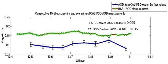
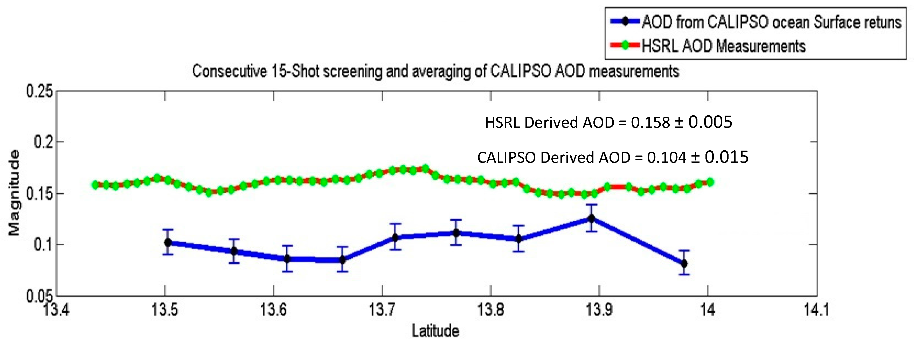
A final example of AOD retrieval along a CALIPSO orbit segment on 22 August 2010 is shown in Figure 19 from combined CALIPSO and under-orbit airborne HSRL measurements during the Caribbean Campaign [16] in August 2010. The NASA Langley airborne HSRL [17] can retrieve the AOD at 532 nm directly by the high spectral resolution lidar (HSRL) technique, providing a truth comparison with the lidar surface return AOD retrieval technique (HSRL uncertainty in AOD retrievals given in Figure 19 is estimated to be <±0.005 based on HSRL retrieval comparisons with both airborne sun-photometer and ground-based AERONET measurements [16], and this is the uncertainty obtained by averaging the HSRL retrievals over the latitude range shown in Figure 19). The shot-by-shot CALIOP AOD retrievals displayed some large spiking (8 of the ~120 shots in the segment), likely due to pre-cloud/cloud-forming effects as is typical of the Caribbean and as seen in the CALIPSO browse image for this segment (which also showed that the aerosol present was likely from an intrusion of dust), so these were screened and a 15-shot (5 km) average was formed for the CALIPSO-derived curve shown in the figure (yielding a standard deviation of ±0.015). The two retrieval curves track fairly well, and their means agree within ~0.05. As CALIPSO passed over this surface segment within seconds, while the HSRL aircraft took upwards of ~15 min to complete the segment, some spatial-temporal variation between the curves could occur (perhaps as seen in the lat region between 13.9 to 14 degrees), although results by Rogers et al. [16] indicate negligible difference should occur due to such a small temporal mismatch. This preliminary result of the lidar surface return AOD retrieval technique being capable of retrieving AOD within ~0.05 is regarded as a good start. It compares favorably with the accuracy first reported by Josset et al. [18] for their retrieval approach using combined CALIPSO and CloudSat ocean surface returns. It is also within the statistically determined difference between CALIPSO-derived AODs, using assumed aerosol models, and HSRL-determined AODs (i.e., standard deviation of CALIPSO model-derived AODs fell within the HSRL AOD determinations for 50% of the comparisons), for many comparisons [16]. However, an additional point to note regarding this comparison is that subsequent investigation of measurements made of flight hardware replicas of the CALIOP detector and post-detection electronics [5], as well as on-orbit investigations of surface return signals [6,7], when examined on a log scale revealed a slight after-pulsing tail on the measured 532 nm impulse response (such after-pulsing is not uncommon in photomultiplier tube (PMT) detectors), which, if included in the impulse response area integration, could bias ${\mathrm{A}}_{\mathrm{LPF}}$ higher and AOD lower. Preliminary investigations to characterize and remove the tail effect by limiting the area determination under the impulse response curve to about the first 400 nanoseconds after the pulse start yielded a higher AOD determination of 0.125 [19], an AOD increase of 0.021 (or an A_LPF area decrease of 4.2%), which brings the tail-corrected AOD (0.125) to about 0.03 below the HSRL AOD retrieval of 0.158.

Another possible effect which can also bias the A_LPF retrieval too high is a contribution from backscattering in the water below the air-water interface. This effect was not assessed in the initially submitted manuscript, but one of the authors (J. Reagan) was made aware of this possible area contribution (by Chris Hostetler) during a visit to NASA Langley Research Center on 3 November 2016. While water is opaque to 1064 nm light, it is slightly transmissive/transparent at 532 nm, although light at this wavelength is largely extinguished within a few tens of meters below the water surface. To estimate the water backscattering area contribution, A_w, in a form directly comparable to the water reflectance contribution, A_LPF, a number of effects must be taken into account. First of all, the total backscattering from the transmitted lidar pulse as it propagates downward in the water is given by the water Total Integrated Attenuated Backscatter, TIAB_w, for an integration in-water distance, z_w, from 0 at the surface to a distance below the surface where backscattering is effectively nil (a few 10 s of meters). Treating the water backscatter, β_w, as effectively constant over the short penetration distance and the water extinction as S_wβ_w, where S_w is the water extinction-to-backscatter ratio, TIAB_w reduces to simply 1/2S_w. As the propagation is in water, the speed of propagation is 2c/n; where n is the water refractive index (1.33), a factor of 2n/c should be multiplied times TIAB_w, analogous to the 2/c term in Equation (5) for A_LPF. A transmission loss occurs as the laser pulse transmits into water and backscatter exits the water because the air-water transmittance, T_aw = (1 − R₅₃₂), is <1, causing an additional loss (1 − R₅₃₂)² to be multiplied times the air round-trip transmittance, T²(z_s). Finally, the backscatter exiting water to air is refracted causing a beam-spreading effect that reduces the radiance seen by the lidar receiver by 1/n². Hence, the A_w contribution to the received lidar signal, directly comparable to A_LPF in Equation (5), is given by

$${\mathrm{A}}_{\mathrm{W}}=\frac{2{\mathrm{nT}}^2\left({\mathrm{z}}_{\mathrm{s}}\right){\left(1-{\mathrm{R}}_{532}\right)}^2{\mathrm{TIAB}}_{\mathrm{W}}}{{\mathrm{n}}^2\mathrm{c}}=\frac{{\mathrm{T}}^2\left({\mathrm{z}}_{\mathrm{s}}\right){\left(1-{\mathrm{R}}_{532}\right)}^2}{{\mathrm{ncS}}_{\mathrm{W}}},$$

(25)

including the result that TIAB_w evaluates to 1/2S_w. The ratio of A_w over A_LPF is then simply

$$\frac{{\mathrm{A}}_{\mathrm{W}}}{{\mathrm{A}}_{\mathrm{LPF}}}=\frac{{\left(1-{\mathrm{R}}_{532}\right)}^2}{2{\mathrm{nS}}_{\mathrm{W}}{\mathrm{R}}_{532}}$$

(26)

Using water parameter values representative of relatively clean open ocean water as given by Churnside [20] and R₅₃₂ for the observation site time (i.e., β_w = ~3 × 10⁻⁴ m⁻¹·sr⁻¹, S_w = 175 sr and R₅₃₂ = ~0.03 sr⁻¹), Equation (5) yields a value of ~0.067 (indicating a 6.7% area enhancement to A_LPF due to water backscatter), indicating the AOD retrieval is biased ~0.034 too low. For the assumed parameter values, the water-attenuated backscatter is reduced effectively to zero (within 0.1%) within two of the 532 nm down-linked samples (within 45 m below the surface), meaning the A_w contribution is effectively captured in the same samples determining A_LPF. Adding both the tail effect and water backscatter biases (0.021 + 0.034 = 0.055) yields a bias-corrected AOD (0.104 + 0.055) of 0.159, almost exactly equal to the HSRL AOD retrieval of 0.158. Allowing for even a ±25% variation in the estimated 0.055 bias (due to some possible variation/uncertainty in the assumed parameters) yields a bias-corrected AOD in the range of 0.145 to 0.173, which still falls within the ±0.015 standard deviation estimated (from the 15-shot averaging) for the initial CALIPSO AOD retrieval value (0.104 ± 0.015). Thus, with bias correction, the HSRL and CALIPSO AOD retrievals are found to agree within <±0.02.

4. Conclusions

A technique has been presented and applied to numerous Cloud-Aerosol Lidar and Infrared Pathfinder Satellite Observation (CALIPSO)/Cloud-Aerosol Lidar with Orthogonal Polarization (CALIOP) observations for estimating from signal samples the normalized area, ${\mathrm{A}}_{\mathrm{LPF}}$, under the received surface response from CALIOP-transmitted lidar pulses reflected from ocean surfaces. An analytic relation for ${\mathrm{A}}_{\mathrm{LPF}}$ has also been developed which shows that this area is proportional to the product of round-trip atmospheric transmission to the ocean surface, ${\mathrm{T}}^2\left({\mathrm{z}}_{\mathrm{s}}\right)$, times the ocean surface backscatter reflectance, ${\mathrm{R}}_{\mathsf{\lambda }}$. The total integrated attenuated backscatter down to the ocean surface (TIAB), one of the CALIPSO data products, was demonstrated to be useful, along with ocean reflectance, for binning the ${\mathrm{A}}_{\mathrm{LPF}}$ estimates into sub-groups with similar properties and for demonstrating that the technique for estimating ${\mathrm{A}}_{\mathrm{LPF}}$ was in very good to excellent agreement with the analytic prediction for clean, aerosol-free cases, defined by TIAB values <0.0125 (indicating ${\mathrm{T}}_{\mathrm{a}}^2$ = ~1.0).

Groupings of ${\mathrm{A}}_{\mathrm{LPF}}$ defined by binning the areas in small increments of TIAB and wind speed (which in turn defined ${\mathrm{R}}_{\mathsf{\lambda }}$ increments using an assumed reflectance model) yielded tightly clustered groups (majority of group ${\mathrm{A}}_{\mathrm{LPF}}$ having percent standard deviations within 12%) with similar statistics for both wavelength channels (532 and 1064 nm) and all three ocean regions that were investigated. Using ${\mathrm{R}}_{\mathsf{\lambda }}$ predicted by the assumed ocean reflectance/wind speed model permitted retrieval of the aerosol round-trip transmittance, ${\mathrm{T}}_{\mathrm{a}}^2$, from the group ${\mathrm{A}}_{\mathrm{LPF}}$ values, and, in turn, the aerosol optical depth, AOD. As shown, the fractional uncertainty in the retrieved ${\mathrm{T}}_{\mathrm{a}}^2$ due to uncertainty in ${\mathrm{A}}_{\mathrm{LPF}}$ equaled the fractional uncertainty in ${\mathrm{A}}_{\mathrm{LPF}}$, while the AOD uncertainty equaled half that. An alternate High/Low method for retrieving ${\mathrm{T}}_{\mathrm{a}}^2$ and AOD from ratios of ${\mathrm{A}}_{\mathrm{LPF}}$ for high and low TIABs, for the same wind speed, was also presented and demonstrated to be in very good agreement with results obtained by the analytic method. From the statistics for the retrieved ${\mathrm{A}}_{\mathrm{LPF}}$, it was estimated that the uncertainty in AOD retrievals from the group ${\mathrm{A}}_{\mathrm{LPF}}$ should be less than ±0.06 in the majority of cases.

Example AOD retrievals presented for two CALIPSO orbit track segments yielded similarly good results with per-shot AOD standard deviations within ±0.05. With multi-shot spatial averaging over a few km (2 to 5 km), the AOD retrieval uncertainty was reduced to <±0.02. One of the cases was concurrent with an under-orbit flight with an HSRL lidar at 532 nm that provided an independent AOD retrieval, and the means of the two 532 nm AOD retrievals were found to agree within 0.05, seemingly too high to be really useful except in cases of high AOD. However, two bias effects (PMT tail effect and underwater backscattering) were identified, both of which produce an enhancement in the data-estimated A_LPF. Applying bias corrections for both of these effects yielded a bias-corrected CALIPSO AOD retrieval within 0.001 of the HSRL AOD retrieval. Allowing for reasonable uncertainty, the bias corrections still yielded a corrected AOD agreeing with the HSRL retrieval within ±0.015, which equals the uncertainty associated with the initial, uncorrected CALIPSO AOD retrieval. Thus, with bias corrections, the technique presented appears capable of retrieving AODs with an accuracy within ~±0.02 (corresponding to an error within ~±4% for the ALPF determination). It should be noted that the retrieval results were for CALIPSO observations over a limited global region (see Figure 14), and results might not be as good over other ocean regions; e.g., due to the lidar calibrations perhaps being more uncertain in regions more poleward. But it should also be noted that the analysis results for the regions investigated did not suggest any significant effect due to lidar calibration error or error in the wind speed model/wind speed input to the model.

The spectral ratio of the aerosol round-trip transmission, ${\mathrm{T}}_{\mathrm{a}1064}^2/{\mathrm{T}}_{\mathrm{a}532}^2$, which can be determined without need of a specific wind speed–reflectance model, was also demonstrated to be useful in validating the expected ratio value for clean, aerosol-free conditions (TIAB < 0.0125), in retrieving the difference in aerosol optical depths (AOD) between the two wavelengths (AOD₅₃₂ − AOD₁₀₆₄), and in providing a parameter potentially useful in aiding/constraining methods for typing aerosols. If AOD is retrieved at both wavelengths, the resulting AOD spectral ratio provides a more direct parameter for aiding aerosol typing. However, given AOD retrieved at just one wavelength, the retrieved spectral ratio of the aerosol round-trip transmission (yielding AOD₅₃₂ − AOD₁₀₆₄) can be used to obtain the AOD at the other wavelength. AOD spectral ratios (532/1064) obtained for the area groups and one of the orbit track segment retrieval examples (9 May 2011) yielded ratios close to/within the range of ratios specified for marine and dust aerosol models (generally agreeing with the aerosol types identified in the CALIPSO browse images).

The results of this investigation, although admittedly preliminary, argue strongly for implementing the technique presented here to retrieve atmospheric AODs from CALIOP ocean surface returns to form a CALIPSO database of global over ocean AOD at both 532 nm and 1064 nm. Such a database would be valuable in itself for monitoring changes in aerosols over time, investigating episodic aerosol events (e.g., dust and smoke layers) and in providing information useful in the development of predictive models of aerosols and their effects on climate. The surface-derived AOD retrievals at 532 nm and 1064 nm can also be used in combination with aerosol typing schemes presently used in producing CALIPSO backscatter and extinction data products to further confirm and enhance these products. The surface-derived spectral AOD information used in conjunction with CALIOP dual-wavelength atmospheric attenuated backscatter should also aid in differentiating aerosol types, or defining additional types, to obtain greater self-consistency between CALIOP profile retrievals and the surface-derived AOD product. The results presented here indicate that AOD retrievals, with bias corrections, may be accurate within ~±0.02, which is sufficient to be quite useful for most observed AODs. To confirm the capability for achieving this level of accuracy, a number of things/effects should be further investigated, particularly before using the technique to produce a CALIPSO global over-ocean data product. These include: modifying the impulse response model to remove the PMT tail effect bias; formulating a correction for the under-water backscattering bias on A_LPF that is easy to implement; investigating possible improvements in the water reflectance model and wind speed estimates used in the model; formulating standard screening/saturated signal-rejection/multi-shot averaging procedures to apply to the data; using improved CALIPSO data product versions (i.e., newly issued version 4); confirming CALIPSO lidar calibration accuracies are sufficient to not significantly bias AOD retrievals in other ocean regions (or flag retrievals in regions where the calibrations are too uncertain), and testing the aforementioned on more CALIPSO data both within and outside the regions investigated in this paper. That said, the results presented here are considered very encouraging and warrant developing (along the lines suggested above) the presented AOD retrieval technique for widespread application.

References

1. Hostetler, C.A.; Liu, Z.; Reagan, J.; Vaughan, M.; Winker, D.; Osborn, M.; Hunt, W.H.; Powell, K.A.; Trepte, C. CALIOP Algorithm Theoretical Basis Document; PC-SCI-201, Release 1.0; National Aeronautics and Space Administration (NASA): Washington, DC, USA, 2006.
2. Winker, D.M.; Vaughan, M.; Omar, A.; Hu, Y.; Powell, K.A. Overview of the CALIPSO mission and CALIOP data processing algorithms. J. Atmos. Ocean. Technol. 2009, 26, 2310–2323. [Google Scholar] [CrossRef]
3. Winker, D.M.; Pelon, J.; Coakley, J.A.; Ackerman, S.A.; Charlson, R.J.; Colarco, P.R.; Flamant, P.; Fu, Q.; Hoff, R.M.; Kittaka, C.; et al. The CALIPSO mission: A global 3D view of aerosols and clouds. Bull. Am. Meteorol. Soc. 2010, 91, 1211–1229. [Google Scholar] [CrossRef]
4. Srikanth, L.V. Aerosol Retrievals from CALIPSO Lidar Ocean Surface Returns. Master’s Thesis, University of Arizona, Tucson, AZ, USA, 2012. [Google Scholar]
5. Hunt, W.; NASA Langley Research Center, Langley, VA, USA. Personal communications, 2012–2014.
6. Hunt, W.H.; Winker, D.M.; Vaughan, M.; Powell, K.; Lucker, P.L.; Weimer, C. CALIPSO lidar description and performance assessment. J. Atmos. Ocean. Technol. 2009, 26, 1214–1228. [Google Scholar] [CrossRef]
7. Hu, Y.; Vaughan, M.A.; Liu, Z.; Lin, B.; Yang, P.; Flittner, D.; Hunt, B.; Kuehn, R.; Huang, J.; Wu, D.; et al. The depolarization-attenuated backscatter relation: CALIPSO lidar measurements vs. theory. Opt. Express 2007, 15, 5327–5332. [Google Scholar] [CrossRef] [PubMed]
8. Reagan, J.A.; Zielinskie, D.A. Space-borne lidar remote sensing techniques aided by surface returns. Opt. Eng. 1991, 30, 96–102. [Google Scholar] [CrossRef]
9. Cox, C.; Munk, W. Measurement of the roughness of the sea surface from photographs of the sun’s glitter. J. Opt. Soc. Am. 1954, 44, 838–850. [Google Scholar] [CrossRef]
10. Kodis, R.D. A note on the theory of scattering from an irregular surface. IEEE Trans. Antennas Propag. 1966, 14, 77–82. [Google Scholar] [CrossRef]
11. Barrick, D.E. Rough surface scattering based on the specular point theory. IEEE Trans. Antennas Propag. 1968, 14, 449–454. [Google Scholar] [CrossRef]
12. Menzies, R.T.; Tratt, D.M.; Hunt, W.H. Lidar in-space technology experiment measurements of sea surface directional reflectance and the link to surface wind speed. Appl. Opt. 1998, 37, 5550–5559. [Google Scholar] [CrossRef] [PubMed]
13. Lancaster, R.S.; Spinhirne, J.D.; Palm, S.P. Laser pulse reflectance of the ocean surface from the GLAS satellite lidar. Geophys. Res. Lett. 2005, 32. [Google Scholar] [CrossRef]
14. Klein, M.V.; Furtak, T.E. Optics, 2nd ed.; John Wiley and Sons: New York, NY, USA, 1986; pp. 80–81. [Google Scholar]
15. Cattrall, C.; Reagan, J.; Thome, K.; Dubovik, O. Variability of aerosol and spectral lidar and backscatter and extinction ratios of key aerosol types derived from selected aerosol robotic network locations. J. Geophys. Res. 2005, 110, D10S11. [Google Scholar] [CrossRef]
16. Rogers, R.R.; Vaughan, M.A.; Hostetler, C.A.; Burton, S.P.; Ferrare, R.A.; Young, S.A.; Hair, J.W.; Obland, M.D.; Harper, D.B.; et al. Looking through the haze: Evaluating the CALIPSO level 2 aerosol optical depth using airborne high spectral resolution lidar data. Atmos. Meas. Tech. 2014, 7, 4317–4340. [Google Scholar] [CrossRef]
17. Hair, J.W.; Hostetler, C.A.; Cook, A.L.; Harper, D.B.; Ferrare, R.A.; Mack, T.L.; Welch, W.; Izquierdo, L.R.; Hovis, F.E. Airborne high spectral resolution lidar for profiling aerosol optical properties. Appl. Opt. 2008, 47, 6734–6752. [Google Scholar] [CrossRef] [PubMed]
18. Josset, D.; Pelon, J.; Protat, A.; Flamant, C. New approach to determine aerosol optical depth from combined CALIPSO and CloudSat ocean surface echoes. Geophys. Res. Lett. 2008, 35. [Google Scholar] [CrossRef] [Green Version]
19. Guilmo, A.; Tyo, J.S.; Reagan, J. CALIOP high resolution IRF modeling based on in-situ observations and application to AOD retrieval. In Presented at 2014 Fall AGU Meeting, San Francisco, CA, USA, 3–5 December 2014.
20. Churnside, J.H.; Sullivan, J.M.; Twardowski, M.S. Lidar extinction to backscatter ratio of the ocean. Opt. Express 2014, 22, 18698–18706. [Google Scholar] [CrossRef] [PubMed]
Figure 1. The impulse response as determined by lab measurements scaled to unity area.
Remotesensing 08 01006 g001
Figure 2. Comparing the two impulse responses. Time is measured in μsec units.
Remotesensing 08 01006 g002
Figure 3. Ocean Surface Reflectance (sr−1) at 532 nm vs. Wind Speed (m/s).
Remotesensing 08 01006 g003
Figure 4. Process of generating down-linked samples for the 532 nm channel.
Remotesensing 08 01006 g004
Figure 5. Process of generating down-linked samples for the 1064 nm channel.
Remotesensing 08 01006 g005
Figure 6. Effect of sampling delay on the down-linked samples for the 532 nm channel.
Remotesensing 08 01006 g006
Figure 7. Effect of sampling delay on the down-linked samples for the 1064 nm channel.
Remotesensing 08 01006 g007
Figure 8. Interpolation results. Sampling delay is plotted in μsec units.
Remotesensing 08 01006 g008
Figure 9. Typical surface return samples at 532 nm and 1064 nm found in the CALIPSO data product.
Remotesensing 08 01006 g009
Figure 10. Showing time instances of the original samples and their average. Time is plotted in μsec units.
Remotesensing 08 01006 g010
Figure 11. Process of scaling in area until the original impulse response of the down-linked sample is recovered: (a) Area scaled too small; (b) Area scaled to fit the down-linked sample. Time is plotted in μsec units.
Remotesensing 08 01006 g011
Figure 12. Impulse response scaled to the final estimated area and the down-linked samples for the 532 nm channel. Time is measured in μsec units.
Remotesensing 08 01006 g012
Figure 13. Impulse response scaled to the final estimated area and the down-linked samples for the 1064 nm channel. Time is measured in μsec units.
Remotesensing 08 01006 g013
Figure 14. The various ocean regions where samples were collected are shown in red, left to right, and a typical night-time orbit (shown in black) passing through each region is included.
Remotesensing 08 01006 g014
Figure 15. Example curve fits showing area values at various TIAB and wind speed values. Also given is number of returns filtered out by the two standard deviation tests.
Remotesensing 08 01006 g015aRemotesensing 08 01006 g015b
Figure 16. Plots showing variation of estimated area with wind speed and TIAB for Southern Pacific Ocean, 532 nm.
Remotesensing 08 01006 g016
Figure 17. Plots showing variation of estimated area with wind speed and TIAB for Southern Pacific Ocean, 1064 nm.
Remotesensing 08 01006 g017
Figure 18. Aerosol round-trip transmission, AOD and TIAB for each retained sample point for 532 nm and 1064 nm channels.
Remotesensing 08 01006 g018
Figure 19. Comparison of CALIPSO ocean surface return and airborne HSRL AOD retrievals.
Remotesensing 08 01006 g019