
Dynamic Water Surface Detection Algorithm Applied on PROBA-V Multispectral Data

Abstract
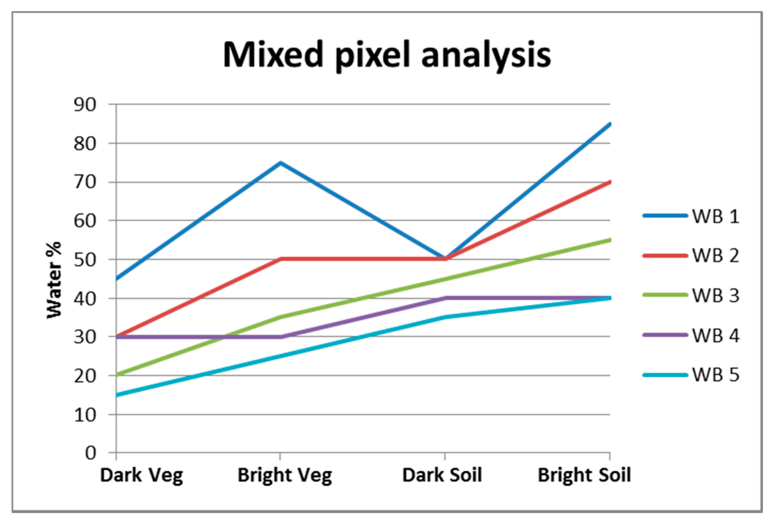
:
1. Introduction
2. Materials and Methods
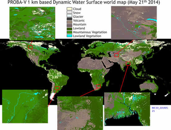
2.1. Overview
2.2. Input Data
2.2.1. Daily Top-Of-Canopy Synthesis Product (S1-TOC)
2.2.2. MC10 Status Map (MC10-SM)
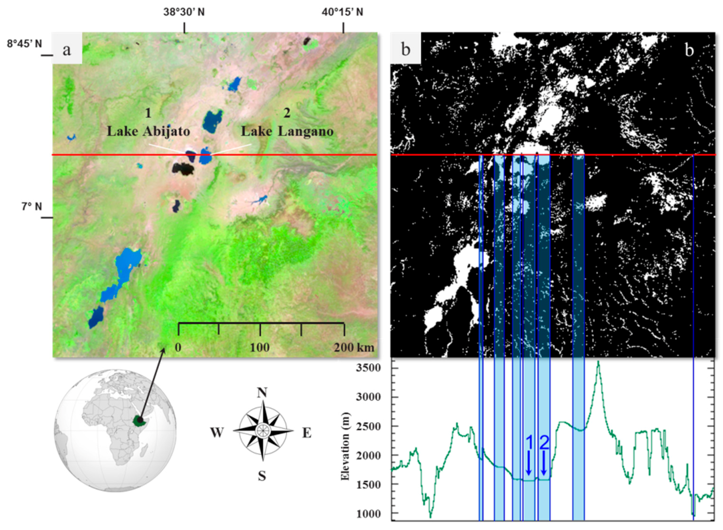
2.2.3. Water Body Potential Mask (WBPM)
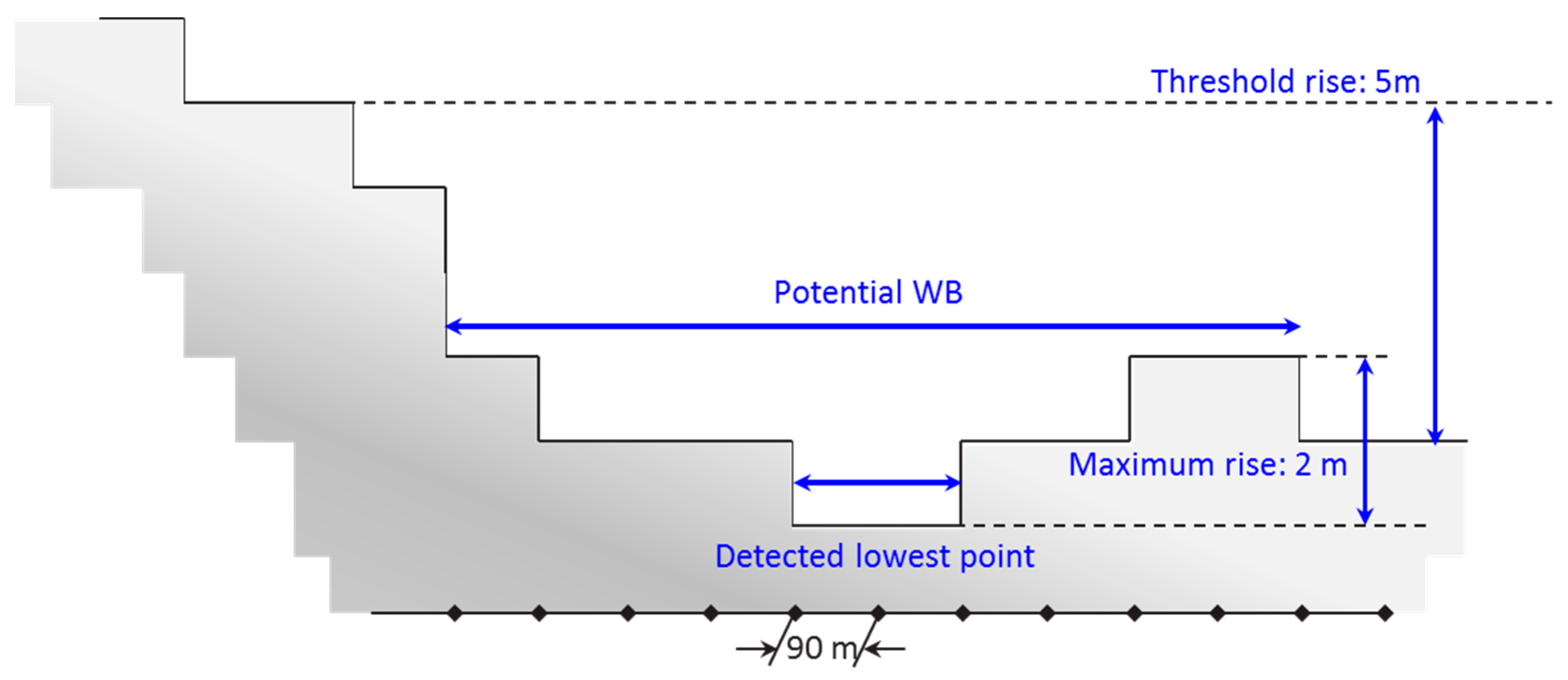
- First the pixels having the lowest elevation in their local neighborhood are located, i.e., a pixel is indicated as a lowest point when its elevation is lower than or equal to its eight neighbors.
- Next, the detected lowest points are filtered and expanded depending on the topography in order to obtain a 90 m spatial resolution potential water body mask. For each detected lowest point, an imaginary water level is raised in steps of 1 m till the maximum rise of 5 m or the flooding condition is reached. Flooding in this context means detection of a neighboring pixel having an elevation that is lower than the rise level. As long as the edge of the potential water body is not flooded, its area is extended according to the raised level, i.e., all neighboring pixels having the additional elevation are added to the potential water body area. This is schematically shown in a two dimensional representation in Figure 2. The initial detected lowest point contains two pixels. Rising the water level 1 m will expand the potential water body with an additional 5 pixels. Because no flooding occurs the water level is increased again with 1 m. Now, an additional 3 pixels are added to the potential water body. Further rising the water level will start flooding the water body because the first pixel elevation right to the expanded water body is lower. If the size of the final expanded water body is less than nine pixels, it is removed from further processing and therefore not considered as a potential water body. Otherwise, the pixels initially detected as lowest point and surrounded by eight neighbors of equal height are marked as level-1. The other initially detected lowest points and the expanded pixels are marked as level-2. The two levels are used in the last step when resizing the potential water body map to the PROBA -V spatial resolution to obtain the final WBPM.
- In the last step, the 90 m spatial resolution potential water body mask is resampled to the PROBA-V 1 km spatial resolution. For each pixel in the georeferenced PROBA-V image, the corresponding pixels in the georeferenced potential water body mask are located. The 1 km resized pixel is indicated as a potential water body when at least one of the corresponding 90 m pixels is labeled as level-1 or when at least nine of the corresponding 90 m pixels are labeled as level-2.
2.2.4. Permanent Glacier Mask (PGM)
2.2.5. Volcanic Soil Mask (VSM)
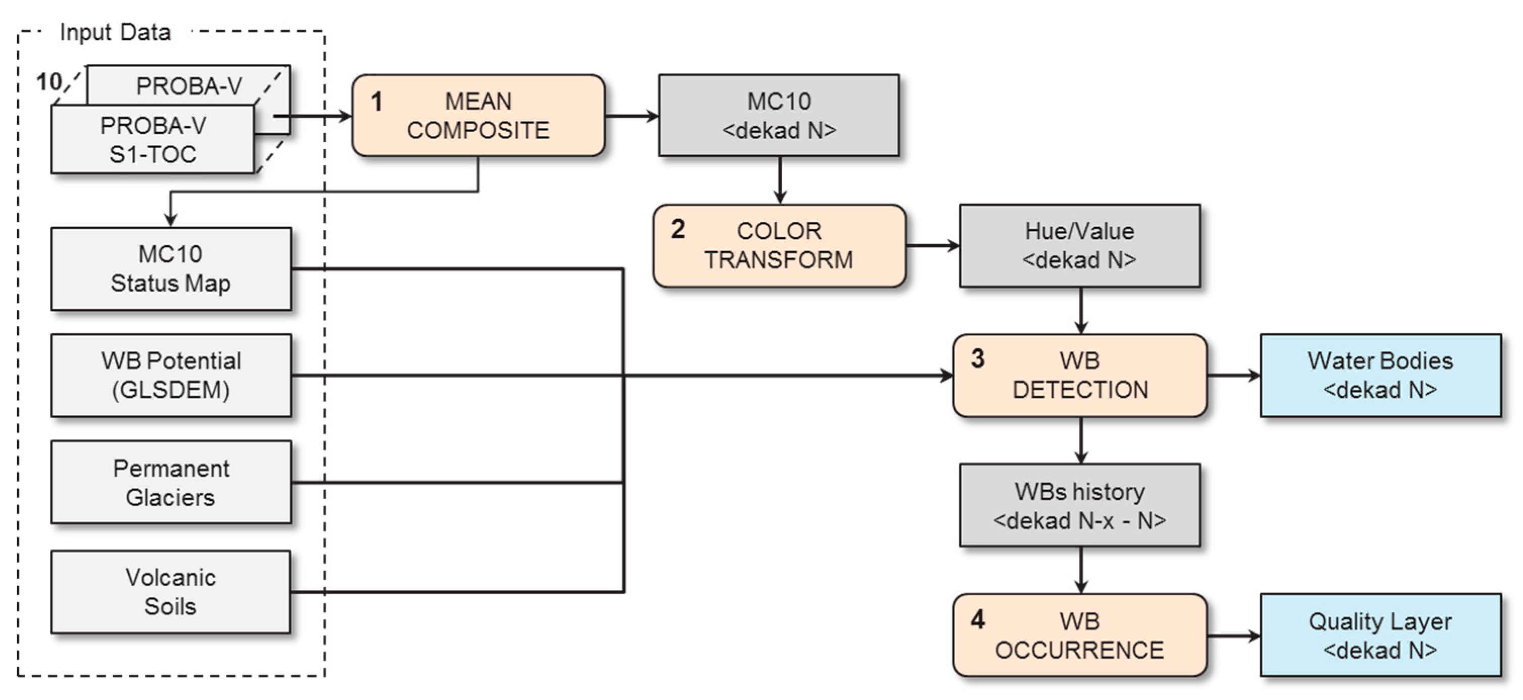
2.3. Mean Compositing
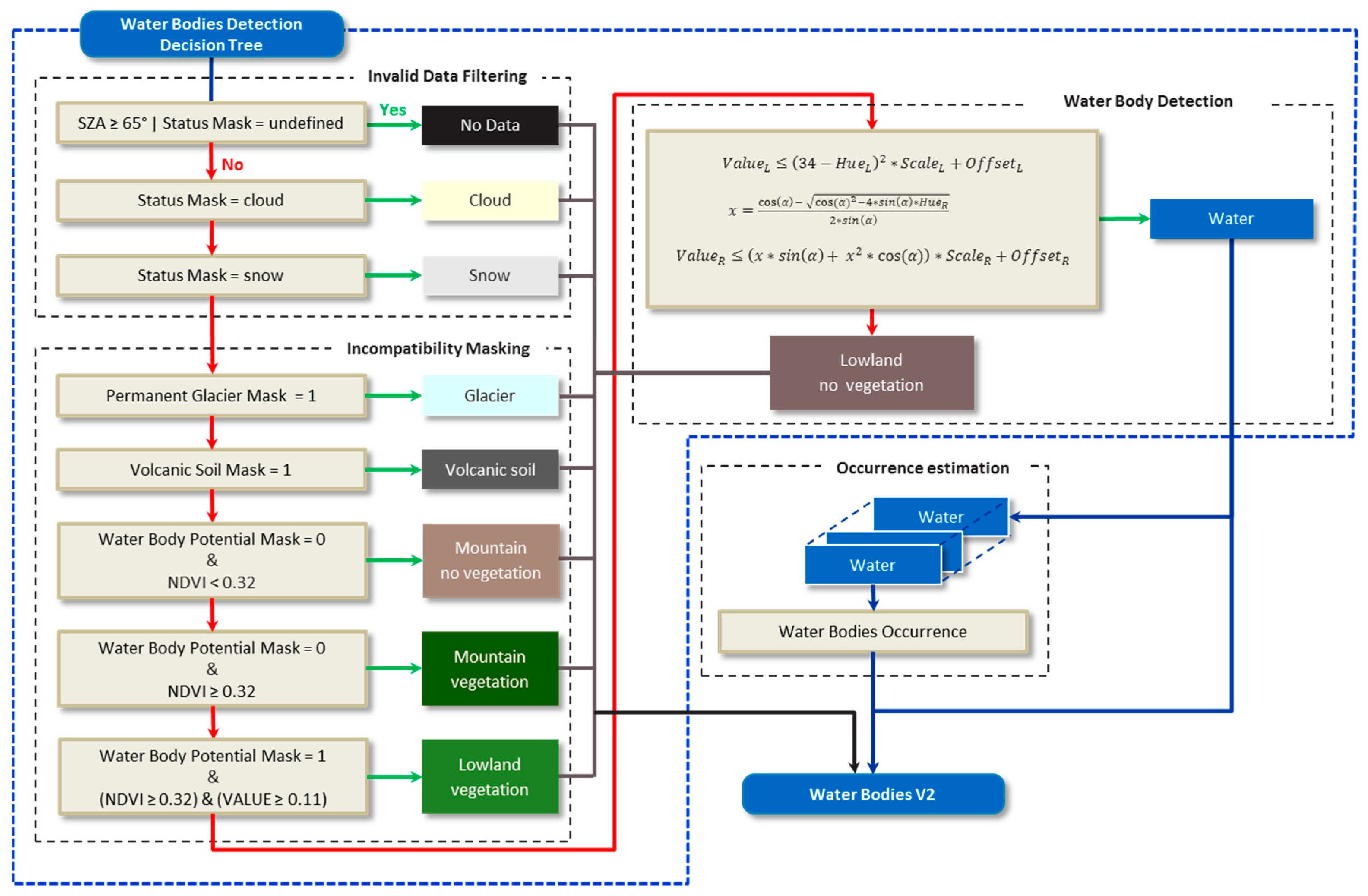
2.4. Water Bodies Detection by Decision Tree Classification
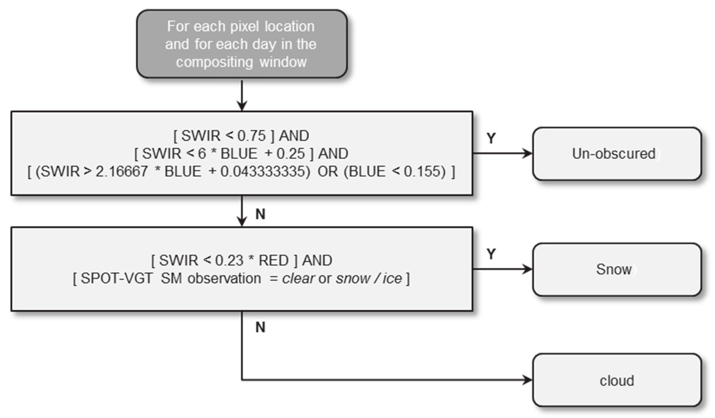
2.4.1. Invalid Data Filtering
2.4.2. Incompatibility Masking
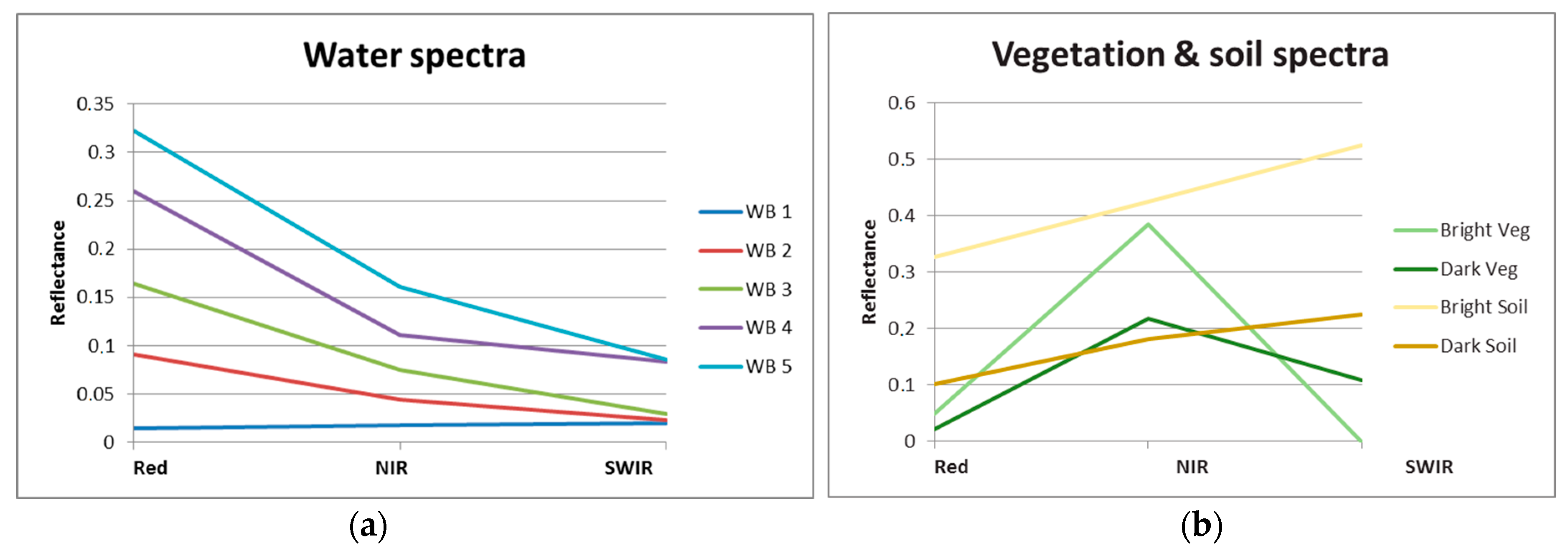
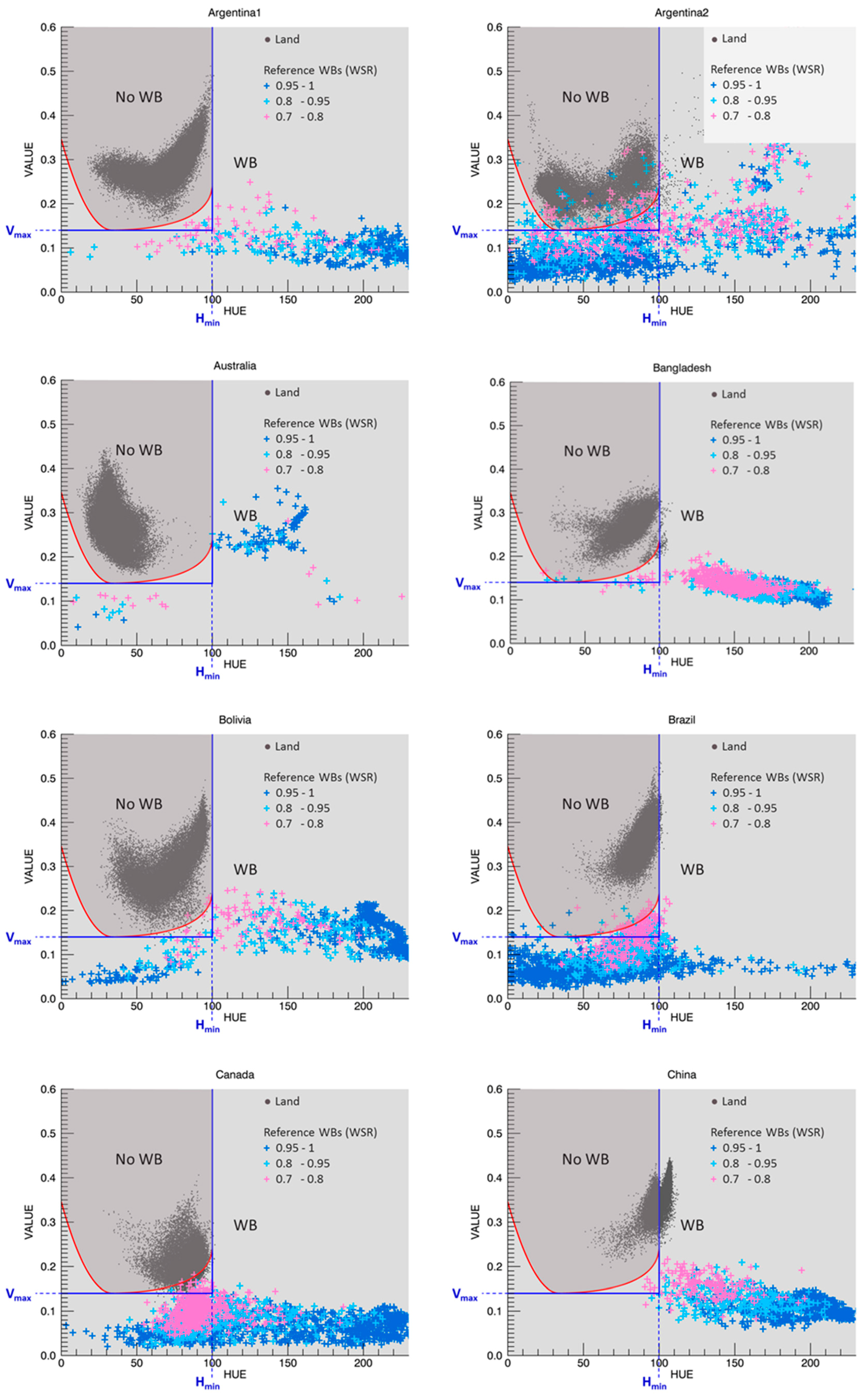
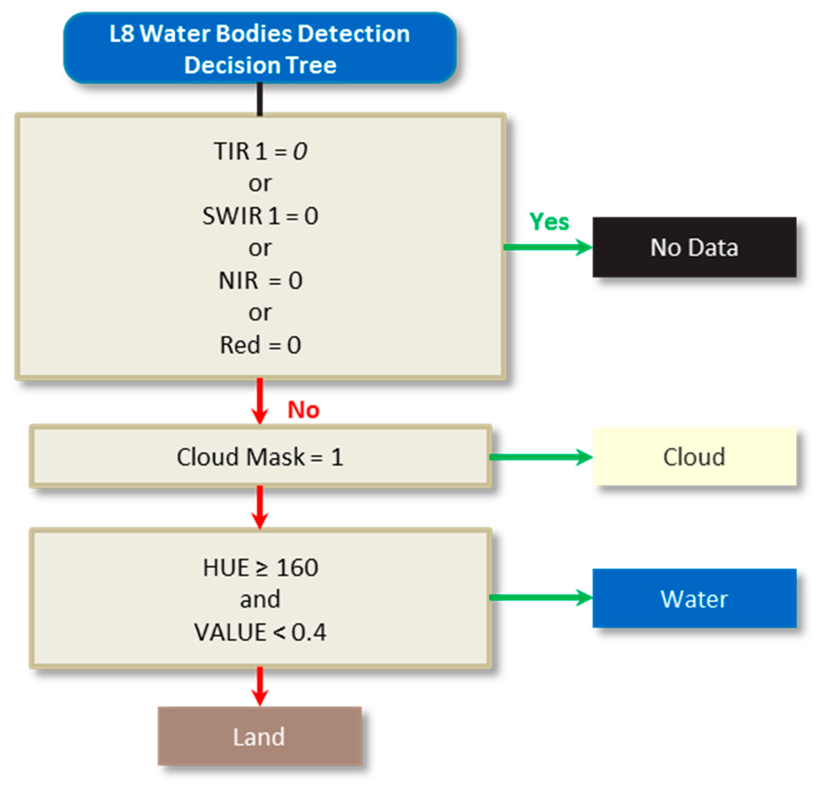
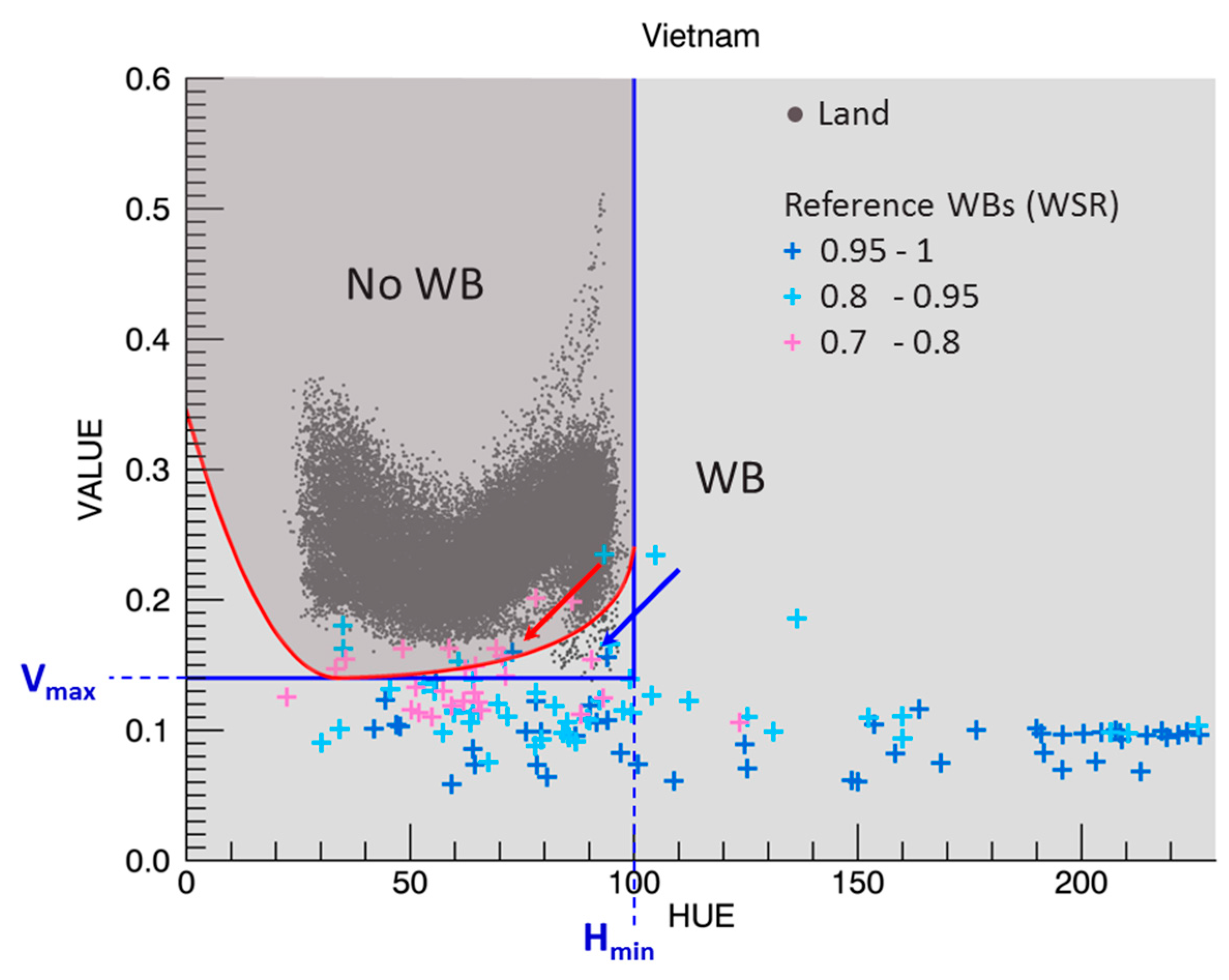
2.4.3. Water Body Detection
- The left part (for the HUE value = 0 till 34) can be written as:
- The right part (for the HUE value = 34 till 100) is a bit more complex because it is based on a parabola rotated over 0.2° for which the rotated coordinates can be written as:This equation can be solved using the standard form:
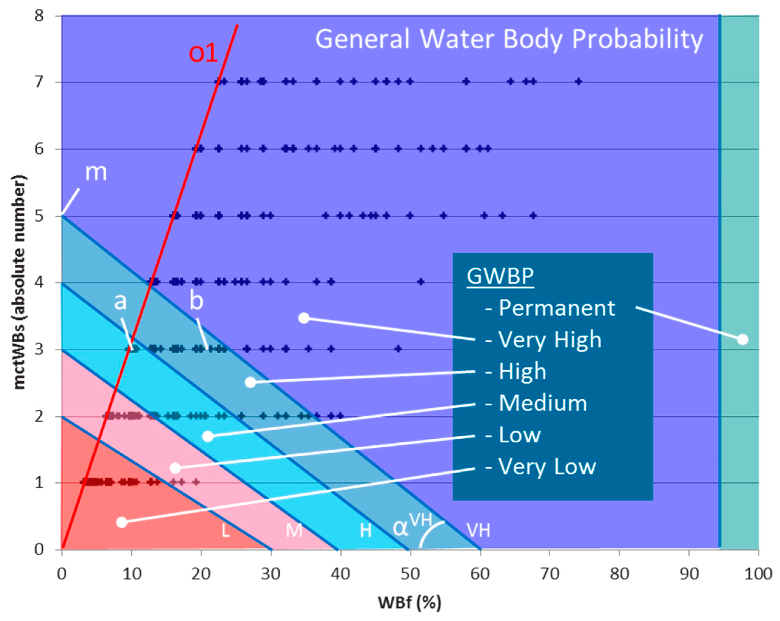
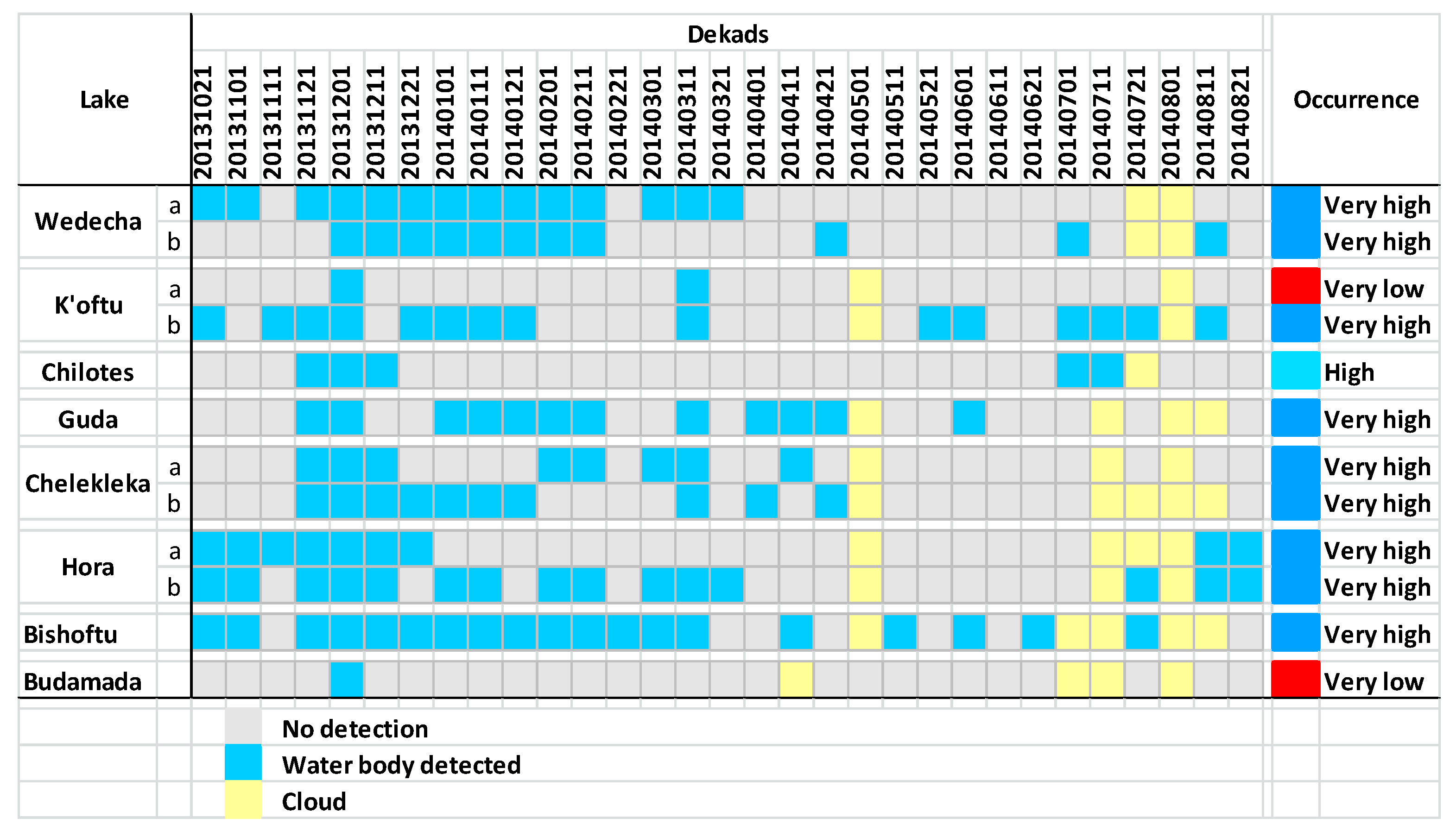
2.5. Water Bodies Occurrence Estimation
- Total number of temporal cloud free observations (ntObs);
- Total number of temporal WB detections (ntWBs); and
- Maximum number of continuous temporal WB detections (mctWBs).
2.6. Minimum Size of Detectable Water Bodies
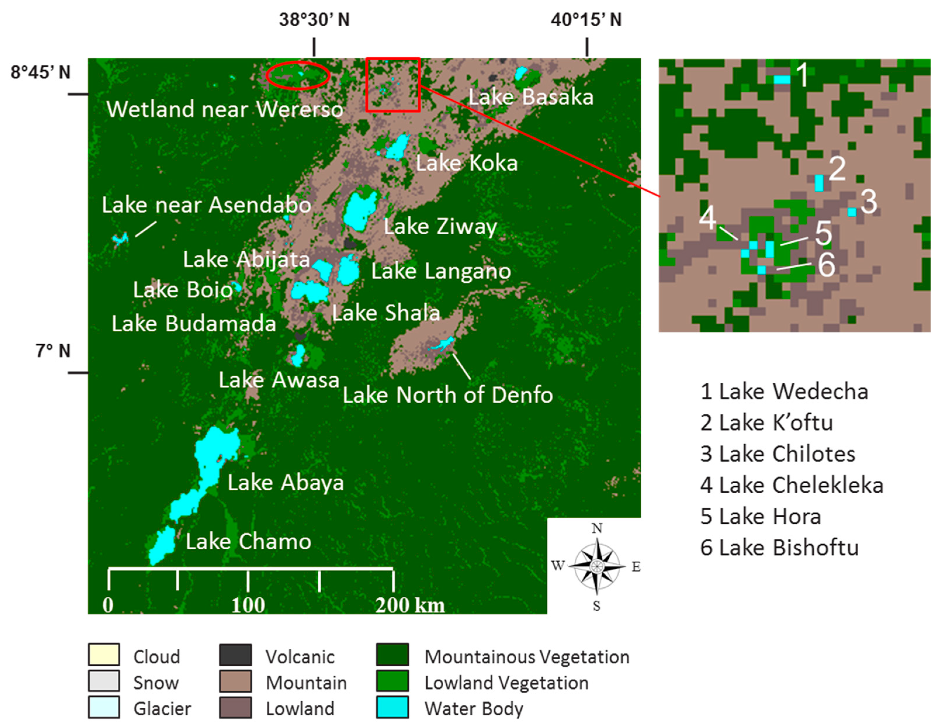
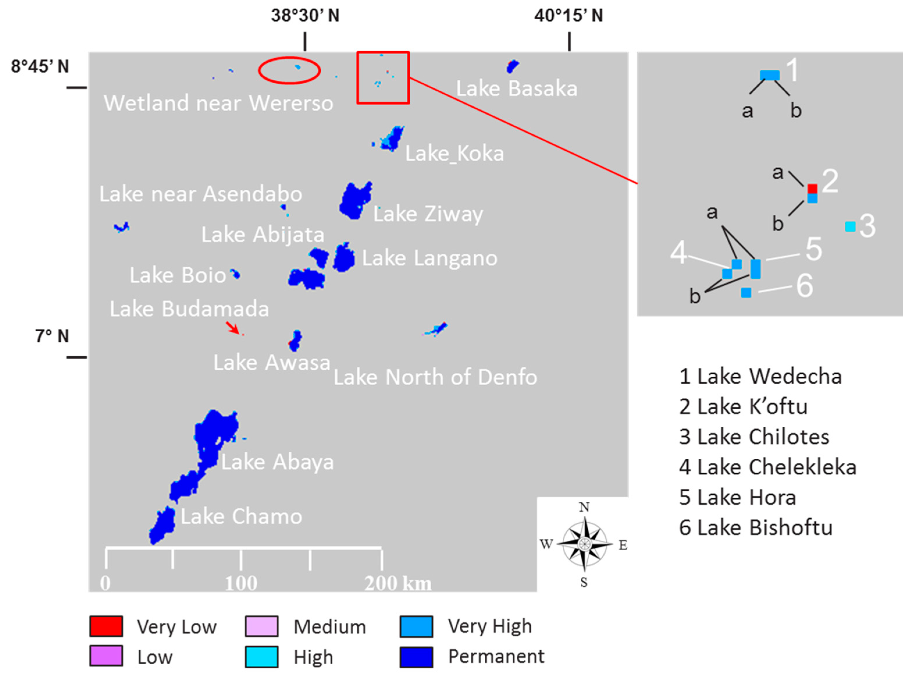
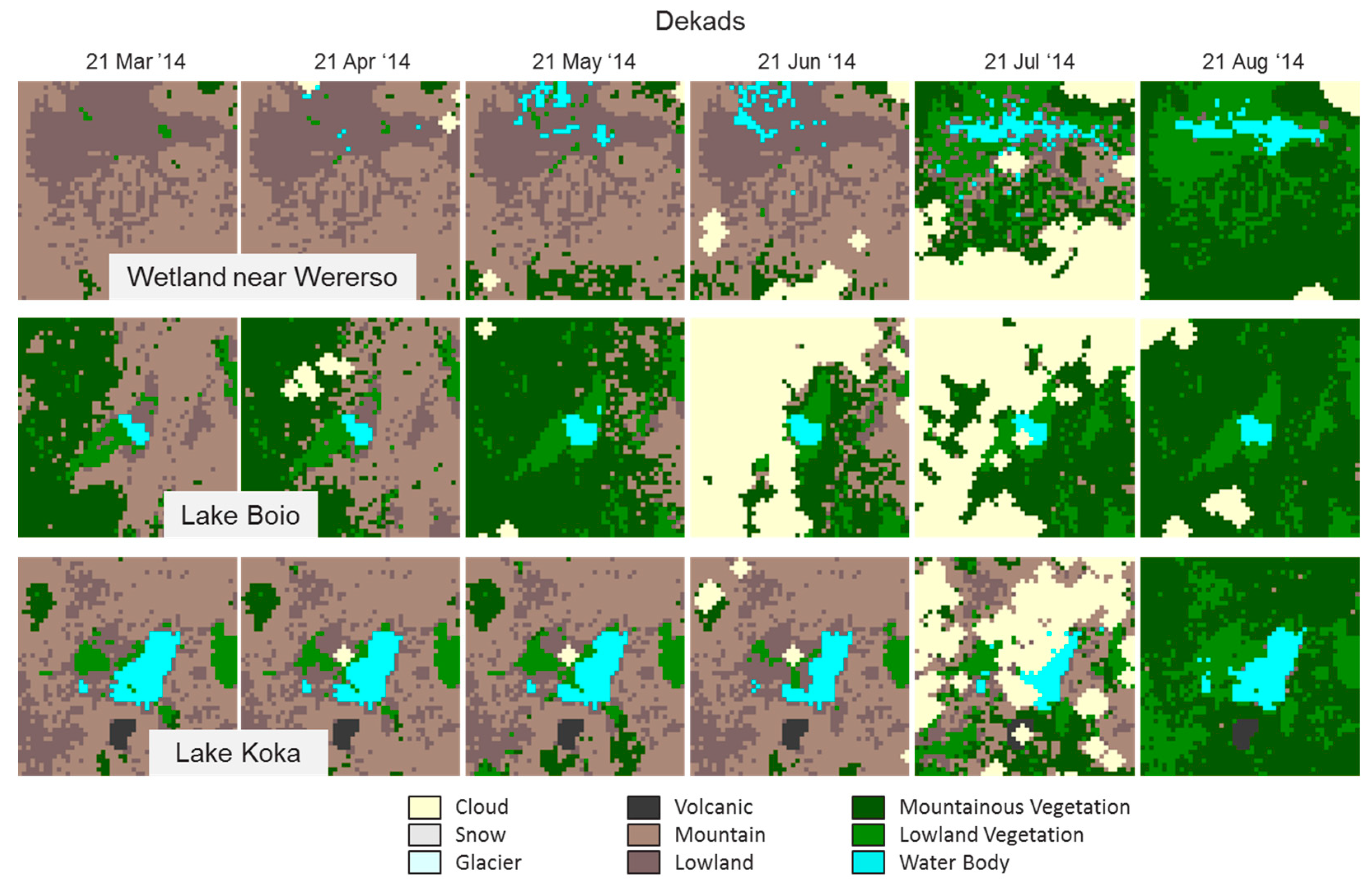
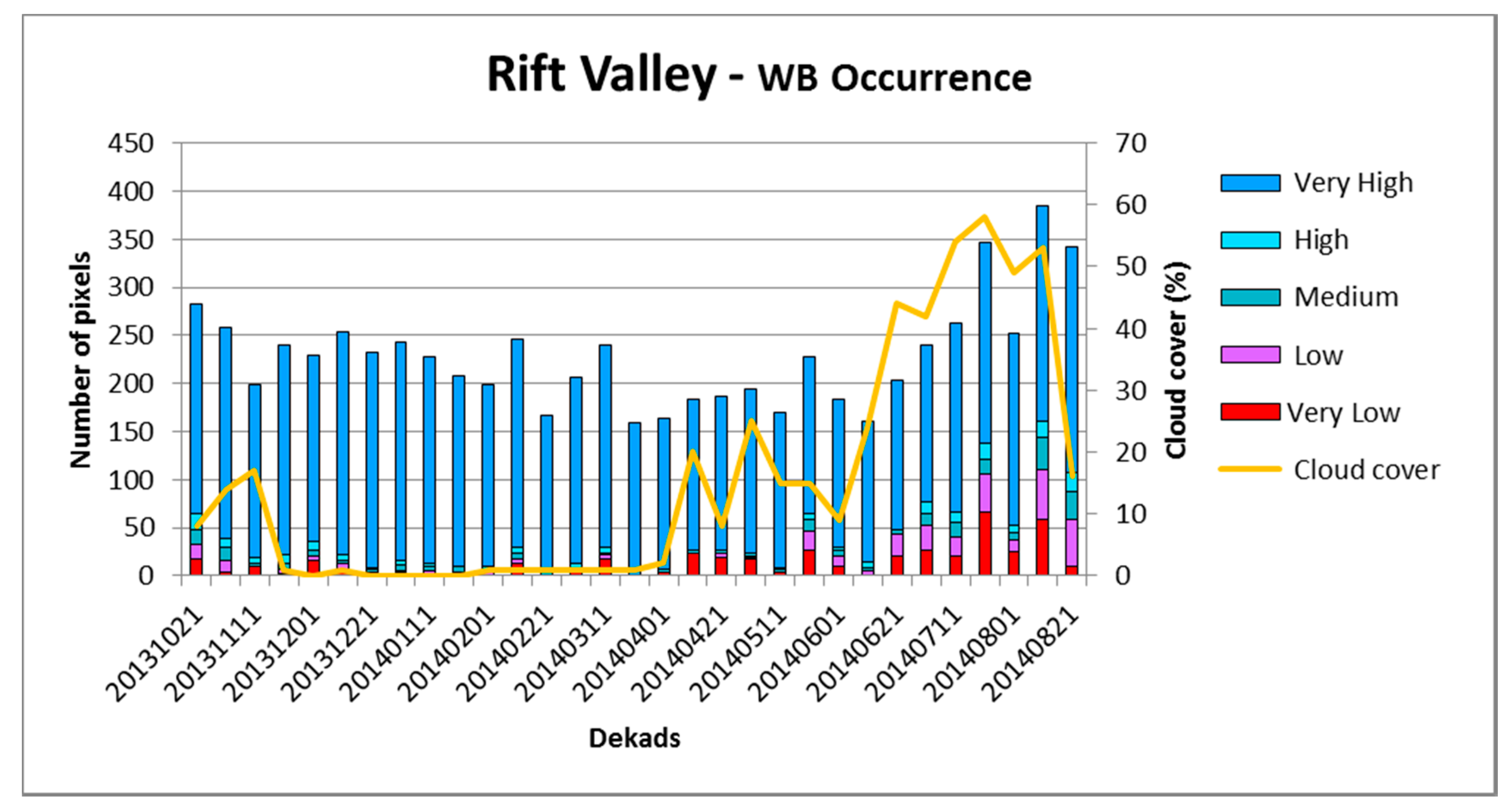
3. Results
4. Assessment of Algorithm Performance
5. Discussion
6. Conclusions
Acknowledgments
Author Contributions
Conflicts of Interest
Appendix A

| Area | Dekad | Upper Left Coordinate | PROBA-V | ||
|---|---|---|---|---|---|
| Lat | Lon | ns | nl | ||
| Rift Valley | 20131201 | 8.96429722 | 37.08032222 | 400 | 400 |
| Area | Landsat 8 Scene | Dekad | Upper Left Coordinate | PROBA-V | ||
|---|---|---|---|---|---|---|
| Lat | Lon | ns | nl | |||
| Argentina 1 | LC82270862014111LGN00 | 20140421 | −36.40625000 | −63.94196429 | 299 | 239 |
| Argentina 2 | LC82310932014011LGN00 | 20140111 | −46.29910714 | −73.83482143 | 376 | 257 |
| Australia | LC81110782014131LGN00 | 20140511 | −24.94196429 | 118.49553571 | 267 | 236 |
| Bangladesh | LC81380442014112LGN00 | 20140421 | 24.17410714 | 87.74553571 | 244 | 240 |
| Bolivia | LC82330692013310LGN00 | 20131101 | −11.95089286 | −66.85267857 | 232 | 239 |
| Brazil | LC82220742014028LGN00 | 20140121 | −19.17410714 | −51.55803571 | 248 | 237 |
| Canada | LC80180272014151LGN00 | 20140521 | 48.53125000 | −80.06696429 | 332 | 246 |
| China | LC81210382014121LGN00 | 20140501 | 32.79910714 | 116.05803571 | 271 | 240 |
| Congo | LC81740662014140LGN00 | 20140521 | −7.62053571 | 25.22767857 | 235 | 238 |
| India | LC81460422014072LGN00 | 20140311 | 27.04910714 | 76.05803571 | 249 | 240 |
| Mali | LC81950502013332LGN00 | 20131121 | 15.51339286 | −2.25446429 | 234 | 239 |
| Mexico | LC80270422014118LGN00 | 20140421 | 27.04017857 | −100.12053571 | 260 | 238 |
| Poland | LC81870222014087LGN00 | 20140401 | 55.60267857 | 21.60267857 | 393 | 250 |
| Rusia | LC81770212014129LGN00 | 20140501 | 56.99553571 | 37.60267857 | 426 | 248 |
| South Africa | LC81690802014121LGN00 | 20140501 | −27.77232143 | 28.12946429 | 277 | 246 |
| Spain | LC82010332014121LGN00 | 20140501 | 39.95089286 | −5.66517857 | 306 | 239 |
| Turkey | LC81730332013306LGN00 | 20131101 | 39.95982143 | 37.65625000 | 299 | 240 |
| USA | LC80430342014134LGN00 | 20140511 | 38.54017857 | −121.87946429 | 281 | 242 |
| Vietnam | LC81240512014062LGN00 | 20140301 | 14.08482143 | 107.11160714 | 241 | 242 |
| Area | Landsat 8 Scene | Dekad | Upper Left Coordinate | PROBA-V | ||
|---|---|---|---|---|---|---|
| Lat | Lon | ns | nl | |||
| Argentina | LC82310872014011LGN00 | 20140111 | −37.83418611 | −70.58413611 | 303 | 241 |
| Australia | LC80950832013304LGN00 | 20131021 | −32.12027778 | 141.27138333 | 288 | 238 |
| Bolivia | LC82330692014233LGN00 | 20140821 | −11.95757500 | −66.85950000 | 233 | 239 |
| Canada | LC80180262014295LGN00 | 20141021 | 49.94476111 | −79.54769167 | 340 | 247 |
| Chad | LC81830512014011LGN00 | 20140111 | 14.06290278 | 15.97345556 | 234 | 238 |
| China | LC81210392014121LGN00 | 20140501 | 31.35326944 | 115.68581667 | 270 | 239 |
| Finland | LC81920132014154LGN00 | 20140601 | 68.02264167 | 21.52997222 | 686 | 253 |
| India | LC81420442014028LGN00 | 20140121 | 24.16315278 | 81.55028611 | 247 | 239 |
| New Zealand | LC80750912014294LGN00 | 20141021 | −43.52644444 | 168.42483889 | 329 | 243 |
| Russia | LC81100132014252LGN00 | 20140901 | 68.03188333 | 148.26286944 | 676 | 255 |
| Swiss | LC81950272014079LGN00 | 20140311 | 48.49976111 | 6.28843889 | 360 | 241 |
| Thailand | LC81280482014090LGN00 | 20140321 | 18.38631389 | 101.85821667 | 247 | 237 |
| Turkmenistan | LC81570332014133LGN00 | 20140511 | 39.95980833 | 62.34785278 | 298 | 242 |
| USA | LC80260372014207LGN00 | 20140721 | 34.21517222 | −96.81486667 | 290 | 237 |
| Zambia | LC81730712014133LGN00 | 20140511 | −14.84697222 | 25.17750000 | 240 | 238 |
Appendix B
Appendix C
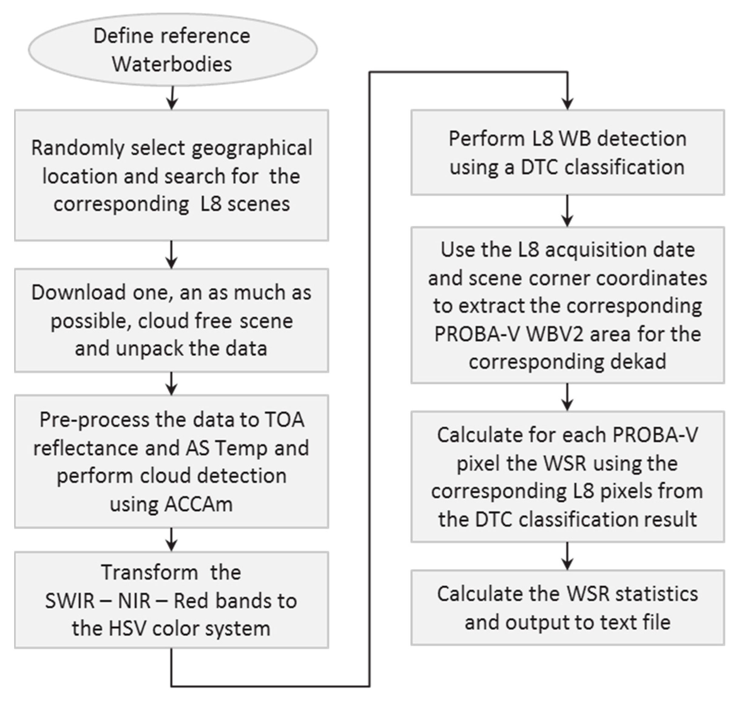
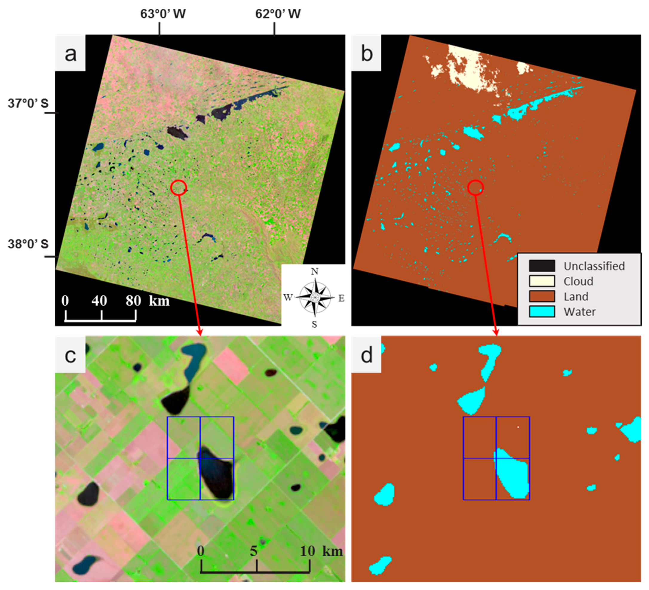
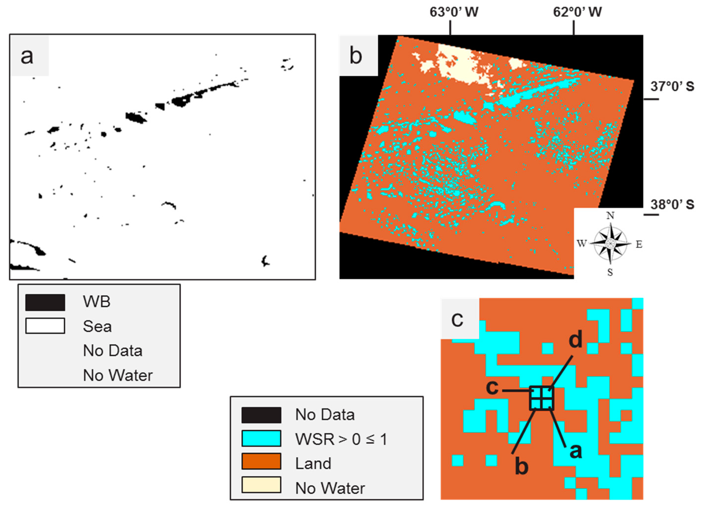
Appendix C.1. Building the Reference Dataset
Appendix C.2. Calculation of the Water Surface Ratio and Evaluation Metrics


| Reference | |||
|---|---|---|---|
| WB | No WB | ||
| WBV2 | WB | p11 | p12 |
| No WB | p21 | p22 | |
- p11 = the number of pixels indicated as WB in both reference and WBV2 and having a WSR larger or equal to the minimum WSR;
- p12 = the number of pixels not indicated as WB in the reference but indicated as WB in WBV2 and having a WSR larger or equal to the minimum WSR;
- p21 = the number of pixels indicated as WB in the reference but not in WBV2 and having a WSR larger or equal to the minimum WSR;
- p22 = the number of pixels not indicated as WB in both reference and WBV2 and having a WSR larger or equal to the minimum WSR.
References
- Vörösmarty, C.J.; Green, P.; Salisbury, J.; Lammers, R.B. Global water resources: Vulnerability from climate change and population growth. Science 2000, 289, 284–288. [Google Scholar] [CrossRef] [PubMed]
- Alsdorf, D.E.; Lettenmaier, D.P. Tracking fresh water from space. Science 2003, 301, 1491–1494. [Google Scholar] [CrossRef] [PubMed]
- Lacaux, J.-P.; Tourre, Y.M.; Vignolles, C.; Ndione, J.-A.; Lafaye, M. Classification of ponds from high-spatial resolution remote sensing: Application to Rift Valley fever epidemics in Senegal. Remote Sens. Environ. 2007, 106, 66–74. [Google Scholar] [CrossRef]
- Breman, H.; Groot, J.J.R.; Van Keulen, H. Resource limitations in Sahelian agriculture. Glob. Environ. Change Hum. Policy Dimens. 2001, 11, 59–68. [Google Scholar] [CrossRef]
- Haas, E.M.; Bartholomé, E.; Combal, B. Time series analysis of optical remote sensing data for the mapping of temporary surface water bodies in sub-Saharan Western Africa. J. Hydrol. 2009, 370, 52–63. [Google Scholar] [CrossRef]
- Hein, L. The impacts of grazing and rainfall variability on the dynamics of a Sahelian rangeland. J. Arid Environ. 2006, 64, 488–504. [Google Scholar] [CrossRef]
- Shevyrnogov, A.P.; Kartushinsky, A.V.; Vysotskaya, G.S. Application of satellite data for investigation of dynamic processes in inland water bodies: Lake Shira (Khakasia, Siberia), a case study. Aquat. Ecol. 2002, 36, 153–164. [Google Scholar] [CrossRef]
- Carroll, M.L.; Townshend, J.R.G.; DiMiceli, C.M.; Loboda, T.; Sohlberg, R.A. Shrinking lakes of the Arctic: Spatial relationships and trajectory of change. Geophys. Res. Lett. 2011, 38, 1–5. [Google Scholar] [CrossRef]
- Cole, J.J.; Prairie, Y.T.; Caraco, N.F.; McDowell, W.H.; Tranvik, L.J.; Striegl, R.G.; Duarte, C.M.; Kortelainen, P.; Downing, J.A.; Middelburg, J.J.; et al. Plumbing the global carbon cycle: Integrating inland waters into the terrestrial carbon budget. Ecosystems 2007, 10, 172–185. [Google Scholar] [CrossRef]
- Craglia, M.; de Bie, K.; Jackson, D.; Pesaresi, M.; Remetey-Fülöpp, G.; Wang, C.; Annoni, A.; Bian, L.; Campbell, F.; Ehlers, M.; et al. Digital Earth 2020: Towards the vision for the next decade. Int. J. Digit. Earth 2012, 5, 4–21. [Google Scholar] [CrossRef]
- Carroll, M.L.; Townshend, J.R.; DiMiceli, C.M.; Noojipady, P.; Sohlberg, R.A. A new global raster water mask at 250 m resolution. Int. J. Digit. Earth 2009, 2, 291–308. [Google Scholar] [CrossRef]
- Klein, I.; Dietz, A.; Gessner, U.; Dech, S.; Kuenzer, C. Results of the Global WaterPack: A novel product to assess inland water body dynamics on a daily basis. Remote Sens. Lett. 2015, 6, 78–87. [Google Scholar] [CrossRef]
- Bartholomé, E. Monitoring the environment in Africa: The VGT4Africa and the AMESD projects. In Proceedings of the 2nd International Workshop on “Crop and Rangeland Monitoring in East Africa”, Nairobi, Kenya, 27–29 March 2007; pp. 303–317.
- Sudheer, K.; Chaubey, I.; Garg, V. Lake water quality assessment from Landsat thematic mapper data using neural network: An approach to optimal band combination selection 1. J. Am. Water Resour. Assoc. 2006, 42, 1683–1695. [Google Scholar] [CrossRef]
- Wang, Y.N.; Huang, F.; Wei, Y.C. Water body extraction from Landsat ETM+ image using MNDWI and KT transformation. In Proceedings of the 21st International Conference on Geoinformatics, Kaifeng, China, 20–22 June 2013.
- Liao, A.; Chen, L.; Chen, J.; He, C.; Cao, X.; Chen, J.; Peng, S.; Sun, F.; Gong, P. High-resolution remote sensing mapping of global land water. Sci. China Earth Sci. 2014, 57, 2305–2316. [Google Scholar] [CrossRef]
- Feng, M.; Sexton, J.O.; Channan, S.; Townshend, J.R. A global, high-resolution (30-m) inland water body dataset for 2000: First results of a topographic-spectral classification algorithm. Int. J. Digit. Earth 2015, 9, 113–133. [Google Scholar] [CrossRef]
- Yamazaki, D.; Trigg, M.A.; Ikeshima, D. Development of a global ~90 m water body map using multi-temporal Landsat images. Remote Sens. Environ. 2015, 171, 337–351. [Google Scholar] [CrossRef] [Green Version]
- Donchyts, G.; Baart, F.; Winsemius, H.; Gorelick, N.; Kwadijk, J.; Giesen, N. Earth’s surface water change over the past 30 years. Nat. Clim. Change 2016, 6, 810–813. [Google Scholar] [CrossRef]
- Ko, B.C.; Kim, H.H.; Nam, J.Y. Classification of potential water bodies using Landsat 8 OLI and a combination of two boosted random forest classifiers. Sensors 2015, 15, 13763–13777. [Google Scholar] [CrossRef] [PubMed]
- Pekel, J.F.; Cottam, A.; Clerici, M.; Belward, A.; Dubois, G.; Bartholome, E.; Gorelick, N. A global scale 30 m water surface detection optimized and validated for Landsat 8. AGU Fall Meet. Abstr. 2014, 1, 01P. [Google Scholar]
- Nath, R.K.; Deb, S.K. Water-body area extraction from high resolution satellite images—An introduction, review, and comparison. Int. J. Image Process. 2010, 3, 353–372. [Google Scholar]
- Sivanpillai, R.; Miller, S.N. Improvements in mapping water bodies using ASTER data. Ecol. Inf. 2010, 5, 73–78. [Google Scholar] [CrossRef]
- Sethre, P.R.; Rundquist, B.C.; Todhunter, P.E. Remote detection of prairie pothole ponds in the Devils Lake Basin, North Dakota. GISci. Remote Sens. 2005, 42, 277–296. [Google Scholar] [CrossRef]
- McFeeters, S.K. The use of the normalized difference water index (NDWI) in the delineation of open water features. Int. J. Remote Sens. 1996, 17, 1425–1432. [Google Scholar] [CrossRef]
- Work, E.A., Jr.; Gilmer, D.S. Utilization of satellite data for inventorying prairie ponds and lakes. Photogramm. Eng. Remote Sens. 1976, 42, 685–694. [Google Scholar]
- Rundquist, D.C.; Lawson, M.P.; Queen, L.P.; Cerveny, R.S. The relationship between summer season rainfall events and lake-surface area. J. Am. Water Resour. Assoc. 1987, 23, 493–508. [Google Scholar] [CrossRef]
- Pekel, J.-F.; Vancutsem, C.; Bastin, L.; Clerici, M.; Vanbogaert, E.; Bartholomé, E.; Defourny, P. A near real-time water surface detection method based on HSV transformation of MODIS multi-spectral time series data. Remote Sens. Environ. 2014, 140, 704–716. [Google Scholar] [CrossRef]
- Bartholomé, E.; Combal, B. VGT4Africa User Manual, 1st ed.; Office for Official Publication of the European Communities: Luxembourg, 2006. [Google Scholar]
- Rahman, H.; Dedieu, G. SMAC: A simplified method for the atmospheric correction of satellite measurements in the solar spectrum. Int. J. Remote Sens. 1994, 15, 123–143. [Google Scholar] [CrossRef]
- Products User Manual. Available online: http://proba-v.vgt.vito.be/ (accessed on 25 May 2016).
- Global Land Cover Facility: 90m Scene GLSDEM_p123r024_utmz13; Global Land Cover Facility, University of Maryland: College Park, Maryland, 2008; Available online: http://glcf.umd.edu/data/glsdem/ (accessed on 17 July 2015).
- Global Land Ice Measurements from Space (GLIMS) Glacier Database; National Snow and Ice Data Center: Boulder CO, USA, 2014; Available online: http://glims.colorado.edu/glacierdata/ (accessed on 28 July 2015).
- Vancutsem, C.; Pekel, J.-F.; Bogaert, P.; Defourny, P. Mean compositing, an alternative strategy for producing temporal syntheses. Concepts and performance assessment for SPOT VEGETATION time series. Int. J. Remote Sens. 2007, 28, 5123–5141. [Google Scholar] [CrossRef]
- GCOS-154. Systematic Observation Requirements for Satellite-Based Products for Climate: Supplemental Details to the Satellite Based Component of the “Implementation Plan for the Global Observing System for Climate in Support of the UNFCCC (2010 Update)”; World Meteorological Organization: Geneva, Switzerland, 2011. [Google Scholar]
- Irish, R.R.; Barker, J.L.; Goward, S.N.; Arvidson, T.J. Characterization of the Landsat-7 ETM+ automated cloud-cover assessment (ACCA) algorithm. Photogramm. Eng. Remote Sens. 2006, 72, 1179–1188. [Google Scholar] [CrossRef]
- Padilla, M.; Stehman, S.V.; Litago, J.; Chuvieco, E. Assessing the temporal stability of the accuracy of a time series of burned area products. Remote Sens. 2014, 6, 2050–2068. [Google Scholar] [CrossRef]
- Roy, D.P.; Boschetti, L. Southern Africa validation of the MODIS, L3JRC, and GlobCarbon burned-area products. IEEE Trans. Geosci. Remote Sens. 2009, 47, 1032–1044. [Google Scholar] [CrossRef]


| Area | CE (%) | OE (%) | |||||
|---|---|---|---|---|---|---|---|
| Minimum WSR | |||||||
| 0.95 | 0.9 | 0.8 | 0.7 | 0.6 | 0.5 | ||
| Argentina | 10.7 | 0 | 0 | 0 | 0 | 0.4 | 0.8 |
| Australia | 1.4 | 0 | 0 | 0 | 0 | 0.8 | 1.1 |
| Bolivia | 0.7 | 0 | 0 | 0.1 | 0.7 | 2.8 | 9.4 |
| Canada | 4.0 | 0 | 0 | 0.2 | 0.3 | 1.5 | 5.0 |
| China | 0 | 0.1 | 0.2 | 0.4 | 1.2 | 3.3 | 7.3 |
| Finland | 1 | 13.6 | 17.3 | 26.8 | 36.3 | 46.6 | 56.2 |
| India | 0 | 0 | 0 | 0 | 1.3 | 7.6 | 16 |
| New Zealand | 0 | 0.2 | 0.2 | 1.4 | 3.9 | 8.1 | 12.3 |
| Russia | 0.1 | 5.3 | 6.9 | 12.2 | 19.0 | 27.6 | 39.8 |
| Swiss | 0 | 0.6 | 1.1 | 3.5 | 6.5 | 11.8 | 18.9 |
| Thailand | 0 | 0 | 0 | 0.4 | 2.2 | 7.4 | 16.9 |
| Chad | 0 | 0 | 0 | 0 | 0 | 0.5 | 1.7 |
| Turkmenistan | 0.3 | 0 | 0 | 0.1 | 0.8 | 2.6 | 6.5 |
| USA | 0 | 0.4 | 0.9 | 6.7 | 14.9 | 24.7 | 32.6 |
| Zambia | 4.9 | 0 | 0 | 0 | 0 | 1.8 | 7.1 |
| Average | 1.5 | 1.3 | 1.8 | 3.5 | 5.8 | 9.8 | 15.4 |
© 2016 by the authors; licensee MDPI, Basel, Switzerland. This article is an open access article distributed under the terms and conditions of the Creative Commons Attribution (CC-BY) license (http://creativecommons.org/licenses/by/4.0/).
Share and Cite
Bertels, L.; Smets, B.; Wolfs, D. Dynamic Water Surface Detection Algorithm Applied on PROBA-V Multispectral Data. Remote Sens. 2016, 8, 1010. https://doi.org/10.3390/rs8121010
Bertels L, Smets B, Wolfs D. Dynamic Water Surface Detection Algorithm Applied on PROBA-V Multispectral Data. Remote Sensing. 2016; 8(12):1010. https://doi.org/10.3390/rs8121010
Chicago/Turabian StyleBertels, Luc, Bruno Smets, and Davy Wolfs. 2016. "Dynamic Water Surface Detection Algorithm Applied on PROBA-V Multispectral Data" Remote Sensing 8, no. 12: 1010. https://doi.org/10.3390/rs8121010