
Preliminary Comparison of Sentinel-2 and Landsat 8 Imagery for a Combined Use


Abstract
:
1. Introduction
2. Materials and Methods
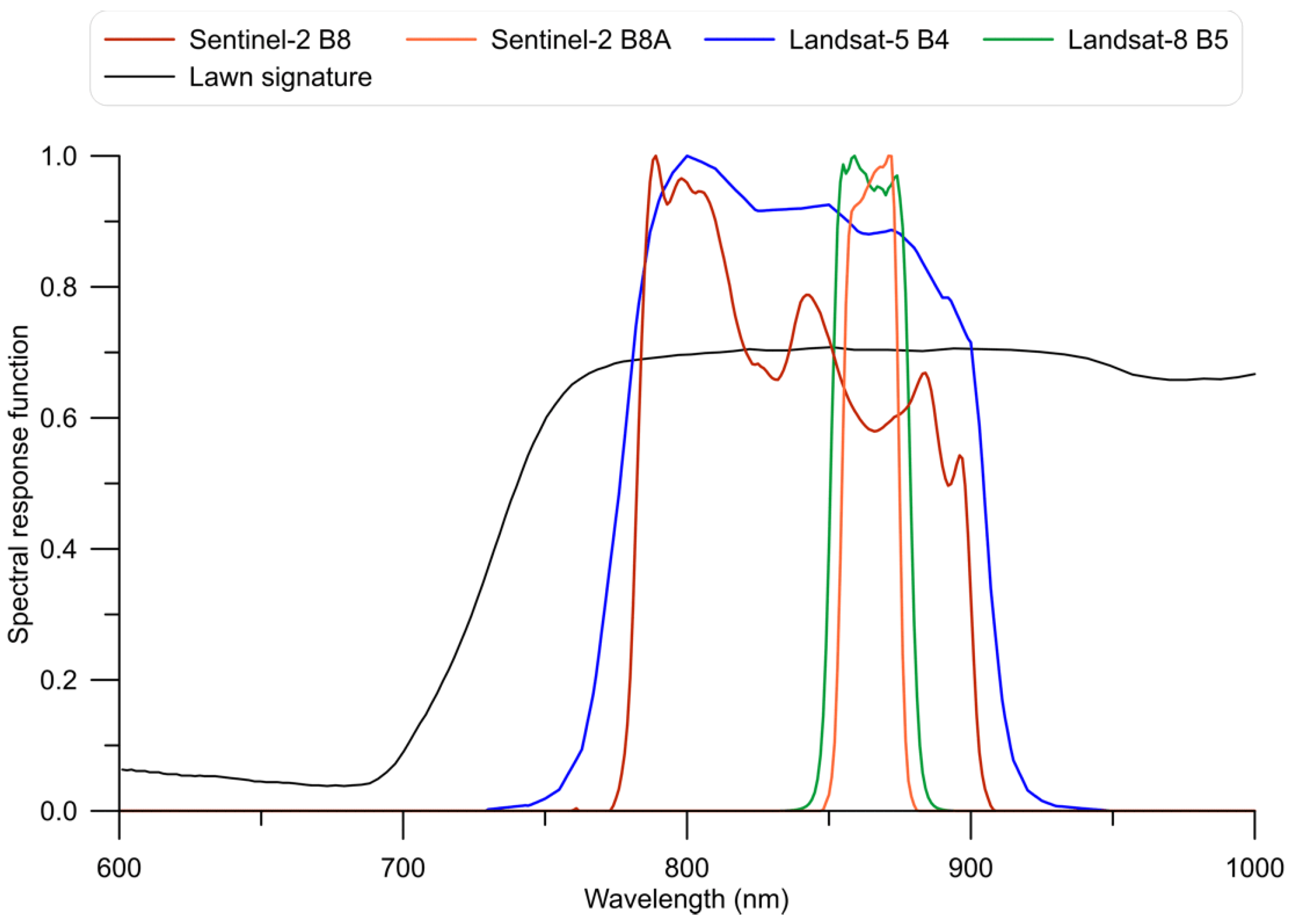
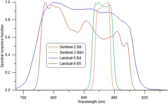
2.1. Simulated Data
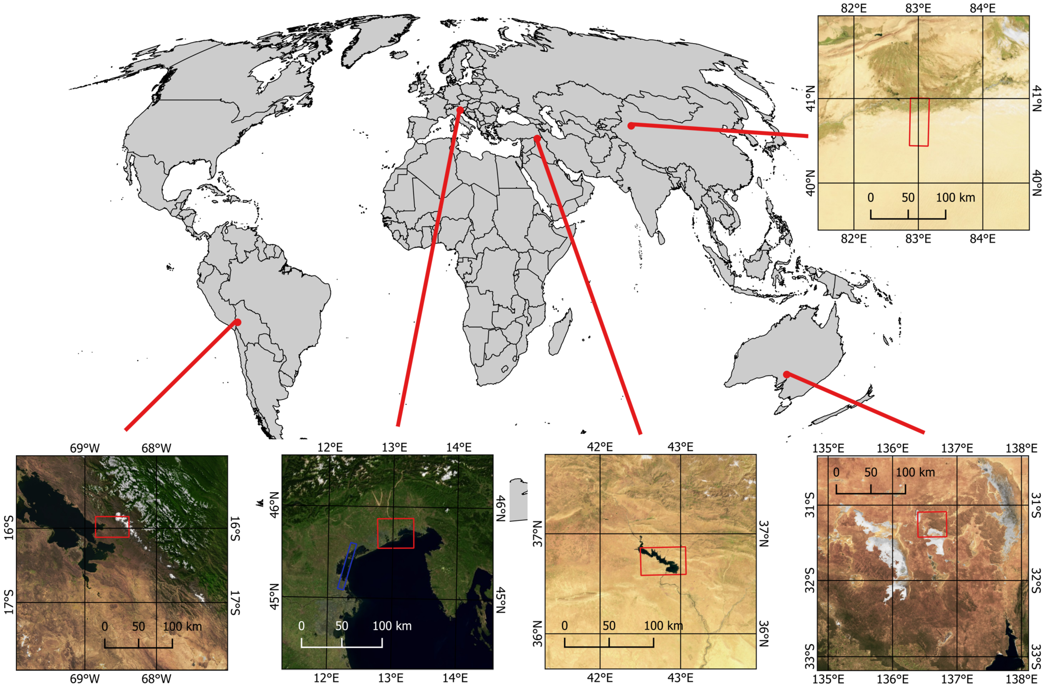
2.2. Real Images
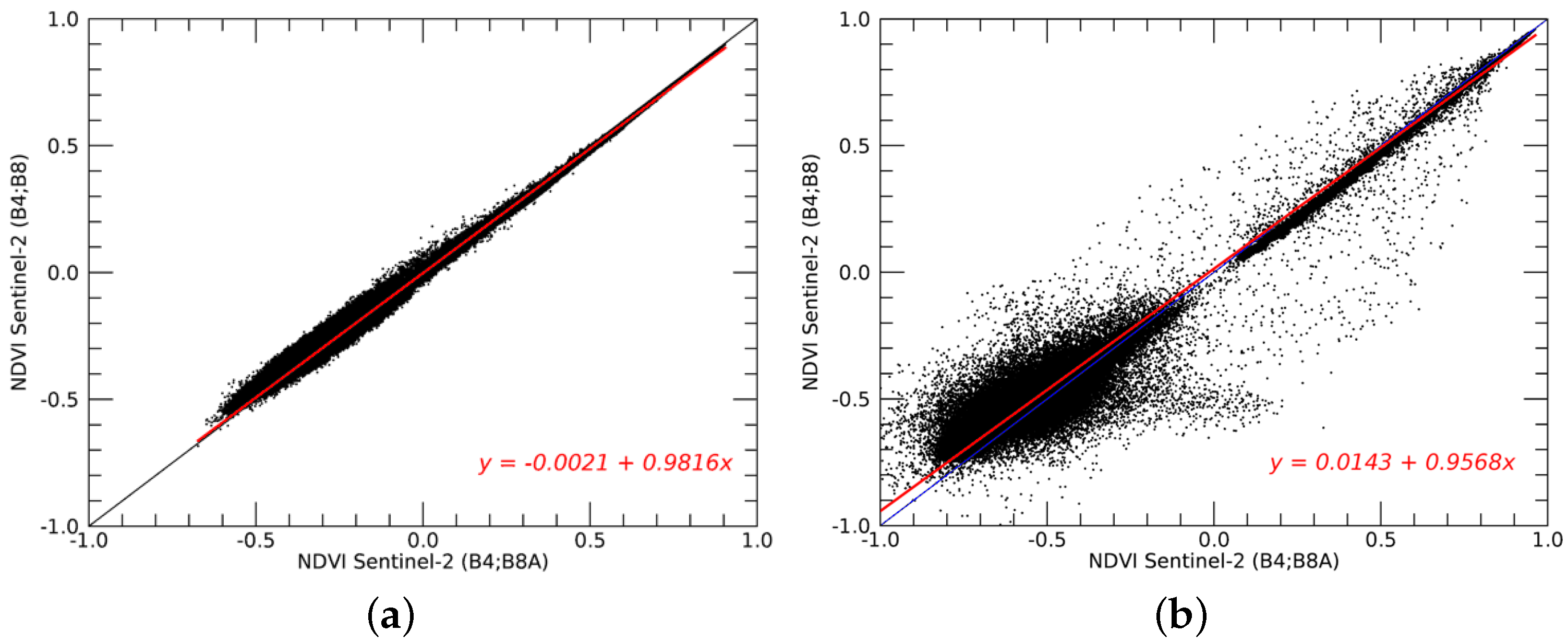
2.3. Sensor Comparison
3. Results and Discussion
4. Conclusions
Author Contributions
Conflicts of Interest
Abbreviations
| B | Band |
| FII | Ferrous Iron Index |
| MSI | Multi-Spectral Instrument |
| NDVI | Normalised Difference Vegetation Index |
| NDWI | Normalised Difference Water Index |
| NIR | Near-Infrared |
| OLI | Operational Land Imager |
| RMSE | Root Mean Square Error |
| RSRF | Relative Spectral Response Function |
| TM | Thematic Mapper |
References
- Hedley, J.; Roelfsema, C.; Koetz, B.; Phinn, S. Capability of the Sentinel 2 mission for tropical coral reef mapping and coral bleaching detection. Remote Sens. Environ. 2012, 120, 145–155. [Google Scholar] [CrossRef]
- Irons, J.R.; Dwyer, J.L.; Barsi, J.A. The next Landsat satellite: The Landsat data continuity mission. Remote Sens. Environ. 2012, 122, 11–21. [Google Scholar] [CrossRef]
- Roy, D.; Wulder, M.; Loveland, T.; Woodcock, C.; Allen, R.; Anderson, M.; Helder, D.; Irons, J.; Johnson, D.; Kennedy, R.; et al. Landsat-8: Science and product vision for terrestrial global change research. Remote Sens. Environ. 2014, 145, 154–172. [Google Scholar] [CrossRef]
- Drusch, M.; Del Bello, U.; Carlier, S.; Colin, O.; Fernandez, V.; Gascon, F.; Hoersch, B.; Isola, C.; Laberinti, P.; Martimort, P.; et al. Sentinel-2: ESA’s optical high-resolution mission for GMES operational services. Remote Sens. Environ. 2012, 120, 25–36. [Google Scholar] [CrossRef]
- Hagolle, O.; Sylvander, S.; Huc, M.; Claverie, M.; Clesse, D.; Dechoz, C.; Lonjou, V.; Poulain, V. SPOT-4 (Take 5): Simulation of Sentinel-2 time series on 45 large sites. Remote Sens. 2015, 7, 12242–12264. [Google Scholar] [CrossRef]
- Kääb, A.; Winsvold, S.; Altena, B.; Nuth, C.; Nagler, T.; Wuite, J. Glacier remote sensing using Sentinel-2. Part I: Radiometric and geometric performance, and application to ice velocity. Remote Sens. 2016, 8. [Google Scholar] [CrossRef]
- D’Odorico, P.; Gonsamo, A.; Damm, A.; Schaepman, M.E. Experimental evaluation of Sentinel-2 spectral response functions for NDVI time-series continuity. IEEE Trans. Geosci. Remote Sens. 2013, 51, 1336–1348. [Google Scholar] [CrossRef]
- Van der Werff, H.; van der Meer, F. Sentinel-2A MSI and Landsat 8 OLI provide data continuity for geological remote sensing. Remote Sens. 2016, 8. [Google Scholar] [CrossRef]
- Lu, D.; Mausel, P.; Brondízio, E.; Moran, E. Change detection techniques. Int. J. Remote Sens. 2004, 25, 2365–2401. [Google Scholar] [CrossRef]
- Mandanici, E.; Bitelli, G. Multi-image and multi-sensor change detection for long-term monitoring of arid environments with Landsat series. Remote Sens. 2015, 7, 14019–14038. [Google Scholar] [CrossRef]
- European Space Agency. Sentinel Website. Available online: https://sentinel.esa.int/documents/247904/685211/Sentinel-2A+MSI+Spectral+Responses (accessed on 28 November 2016).
- National Aeronautics and Space Administration. Landsat Science. Available online: http://landsat.gsfc.nasa.gov/wp-content/uploads/2014/09/Ball_BA_RSR.v1.2.xlsx (accessed on 28 November 2016).
- Jupp, D.L.B.; Datt, B. Evaluation of Hyperion Performance at Australian Hyperspectral Calibration and Validation Sites; CSIRO Earth Observation Centre Report; CSIRO Earth Observation Centre: Canberra, Australia, 2004. [Google Scholar]
- Mandanici, E. Implementation of Hyperion sensor routine in 6SV radiative transfer code. In Proceedings of the Hyperspectral Workshop 2010, Frascati, Italy, 17–18 March 2010; Lacoste-Francis, H., Ed.; ESA: Frascati, Italy, 2010; Volume SP-683. [Google Scholar]
- Kotchenova, S.Y.; Vermote, E.F.; Matarrese, R.; Klemm, F.J.J. Validation of a vector version of the 6S radiative transfer code for atmospheric correction of satellite data. Part I: Path radiance. Appl. Opt. 2006, 45, 6762–6774. [Google Scholar] [CrossRef] [PubMed]
- Bitelli, G.; Mandanici, E. Atmospheric correction issues for water quality assessment from remote sensing: The case of Lake Qarun (Egypt). Proc. SPIE 2010, 7831. [Google Scholar] [CrossRef]
- Yan, L.; Roy, D.; Zhang, H.; Li, J.; Huang, H. An automated approach for sub-pixel registration of Landsat-8 Operational Land Imager (OLI) and Sentinel-2 Multi Spectral Instrument (MSI) imagery. Remote Sens. 2016, 8. [Google Scholar] [CrossRef]
- Mc Feeters, S.K. The use of the Normalized Difference Water Index (NDWI) in the delineation of open water features. Int. J. Remote Sens. 1996, 17, 1425–1432. [Google Scholar] [CrossRef]
- Kalinowski, A.; Oliver, S. ASTER Mineral Index Processing Manual, Remote Sensing Applications; Geoscience Australia: Canberra, Australia, 2004. [Google Scholar]
- Vuolo, F.; Żóltak, M.; Pipitone, C.; Zappa, L.; Wenng, H.; Immitzer, M.; Weiss, M.; Baret, F.; Atzberger, C. Data service platform for Sentinel-2 surface reflectance and value-added products: System use and examples. Remote Sens. 2016, 8. [Google Scholar] [CrossRef]
- Novelli, A.; Aguilar, M.A.; Nemmaoui, A.; Aguilar, F.J.; Tarantino, E. Performance evaluation of object based greenhouse detection from Sentinel-2 MSI and Landsat 8 OLI data: A case study from Almería (Spain). Int. J. Appl. Earth Obs. Geoinf. 2016, 52, 403–411. [Google Scholar] [CrossRef]


| Date | MSI Time | OLI Time | Height (m) | Sun Zenith | Land Cover | |
|---|---|---|---|---|---|---|
| Australia | 4 November 2016 | 00:57 | 00:45 | 100 | 30.1 | Desert and salt lakes |
| Bolivia | 16 July 2016 | 14:52 | 14:35 | 4100 | 45.6 | Bare soils, lakes, crops, snow |
| China | 19 September 2016 | 05:09 | 05:21 | 960 | 42.4 | Sandy desert, lakes, crops |
| Iraq | 16 July 2016 | 7:48 | 7:45 | 350 | 22.3 | Lake, bare soils, crops |
| Italy | 4 August 2016 | 10:06 | 9:52 | 5 | 31.9 | Crops, urban areas, sea |
| Bands | Test Area | Linear Regression | Correlation Pearson Coefficient | ||
|---|---|---|---|---|---|
| MSI Band | OLI Band | Intercept | Slope | ||
| Australia | −0.0057 | 1.0203 | 0.9993 | ||
| Bolivia | −0.0044 | 0.9704 | 0.9981 | ||
| 1 | 1 | China | 0.0042 | 0.9560 | 0.9851 |
| Iraq | −0.0043 | 1.0910 | 0.9825 | ||
| Italy | 0.0022 | 0.9667 | 0.9752 | ||
| Italy (simulated) | −0.0012 | 0.9928 | 0.9995 | ||
| Australia | 0.0013 | 1.0244 | 0.9993 | ||
| Bolivia | 0.0004 | 0.9862 | 0.9979 | ||
| 2 | 2 | China | 0.0071 | 1.0182 | 0.9937 |
| Iraq | −0.0072 | 1.1737 | 0.9868 | ||
| Italy | 0.0016 | 1.0542 | 0.9836 | ||
| Italy (simulated) | 0.0041 | 1.0726 | 0.9989 | ||
| Australia | −0.0088 | 1.0240 | 0.9990 | ||
| Bolivia | −0.0026 | 0.9663 | 0.9972 | ||
| 3 | 3 | China | 0.0020 | 0.9728 | 0.9944 |
| Iraq | −0.0050 | 1.0382 | 0.9919 | ||
| Italy | 0.0000 | 1.0019 | 0.9928 | ||
| Italy (simulated) | 0.0032 | 0.9822 | 0.9992 | ||
| Australia | −0.0038 | 1.0379 | 0.9969 | ||
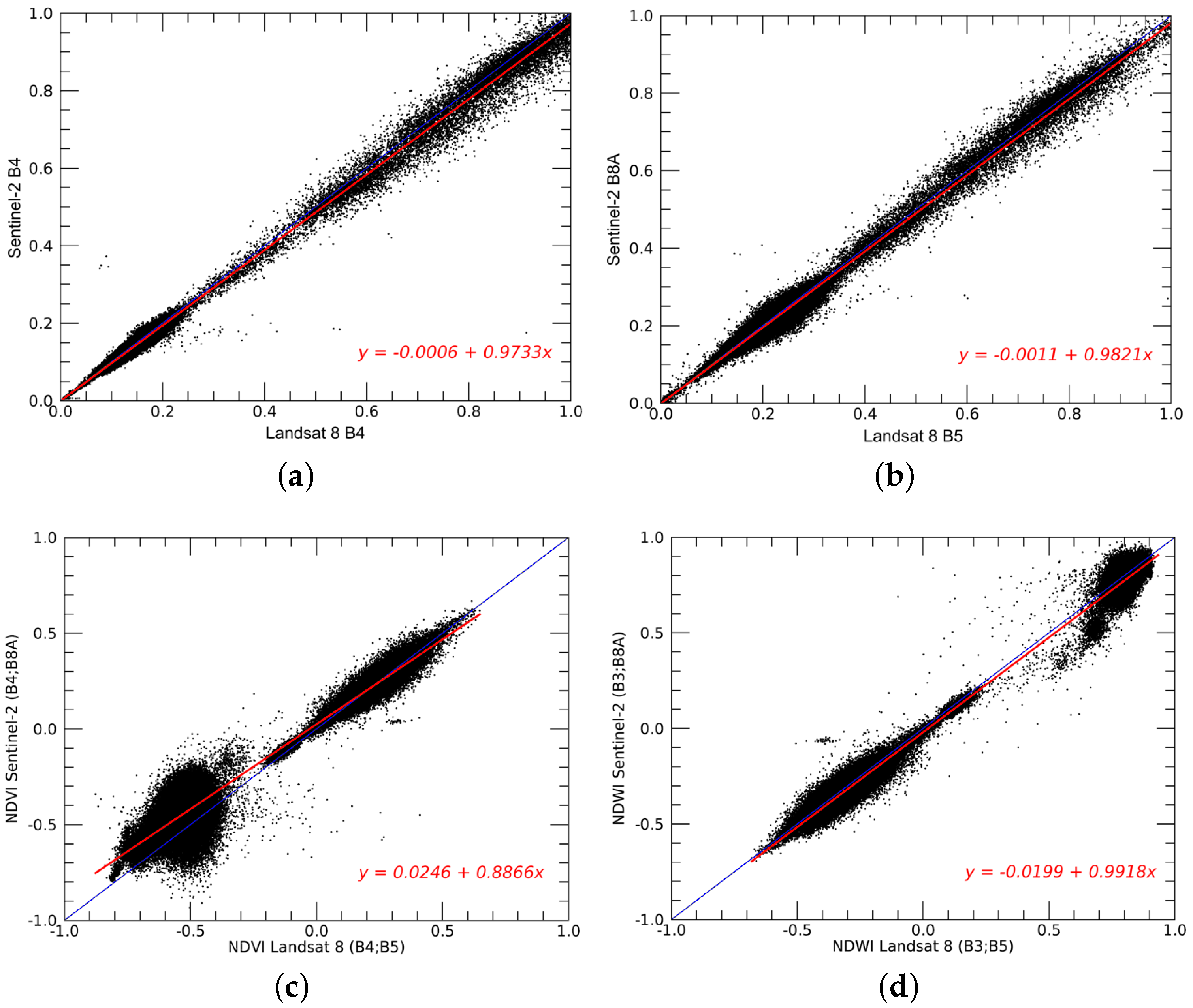
| Bolivia | −0.0006 | 0.9733 | 0.9969 | ||
| 4 | 4 | China | −0.0009 | 0.9728 | 0.9952 |
| Iraq | −0.0061 | 1.0766 | 0.9952 | ||
| Italy | −0.0017 | 1.0376 | 0.9961 | ||
| Italy (simulated) | −0.0020 | 1.0050 | 0.9997 | ||
| Australia | −0.0235 | 1.1198 | 0.9856 | ||
| Bolivia | −0.0016 | 0.9159 | 0.9875 | ||
| 8 | 5 | China | −0.0002 | 0.9595 | 0.9853 |
| Iraq | −0.0028 | 1.0361 | 0.9962 | ||
| Italy | 0.0005 | 0.9648 | 0.9992 | ||
| Italy (simulated) | 0.0018 | 0.9491 | 0.9998 | ||
| Australia | −0.0148 | 1.0675 | 0.9945 | ||
| Bolivia | −0.0011 | 0.9821 | 0.9950 | ||
| 8A | 5 | China | 0.0023 | 1.0015 | 0.9967 |
| Iraq | −0.0035 | 1.0508 | 0.9970 | ||
| Italy | 0.0003 | 1.0248 | 0.9989 | ||
| Italy (simulated) | −0.0001 | 1.0005 | 1.0000 | ||
| Australia | 0.0148 | 1.0162 | 0.9977 | ||
| Bolivia | 0.0034 | 1.0115 | 0.9944 | ||
| 11 | 6 | China | 0.0030 | 1.0459 | 0.9981 |
| Iraq | −0.0043 | 1.1015 | 0.9975 | ||
| Italy | 0.0008 | 1.0824 | 0.9983 | ||
| Italy (simulated) | 0.0001 | 1.0083 | 1.0000 | ||
| Australia | 0.0123 | 1.0313 | 0.9977 | ||
| Bolivia | 0.0034 | 1.0255 | 0.9930 | ||
| 12 | 7 | China | 0.0025 | 1.0624 | 0.9984 |
| Iraq | −0.0029 | 1.1298 | 0.9959 | ||
| Italy | 0.0003 | 1.1022 | 0.9981 | ||
| Italy (simulated) | 0.0002 | 1.0055 | 1.0000 | ||
| Bands | Linear Regression | Correlation Pearson Coefficient | ||
|---|---|---|---|---|
| MSI Band | TM5 Band | Intercept | Slope | |
| 2 | 1 | 0.0031 | 1.0584 | 0.9995 |
| 3 | 2 | 0.0083 | 0.9399 | 0.9962 |
| 4 | 3 | −0.0017 | 1.0001 | 0.9997 |
| 8 | 4 | 0.0001 | 1.0002 | 1.0000 |
| 8a | 4 | −0.0018 | 1.0540 | 0.9998 |
| 11 | 5 | 0.0002 | 1.0284 | 0.9998 |
| 12 | 7 | 0.0004 | 1.0464 | 0.9996 |
| Index | Bands Exploited | Test Area | Linear Regression | Correlation Pearson Coefficient | ||
|---|---|---|---|---|---|---|
| MSI | OLI | Intercept | Slope | |||
| Australia | 0.0055 | 0.9178 | 0.9875 | |||
| Bolivia | 0.0246 | 0.8866 | 0.9862 | |||
| NDVI | 4, 8A | 4, 5 | China | 0.0045 | 0.9820 | 0.9364 |
| Iraq | −0.0120 | 1.0215 | 0.9804 | |||
| Italy | 0.0378 | 0.9301 | 0.9826 | |||
| Italy (simulated) | 0.0039 | 0.9950 | 0.9999 | |||
| Australia | −0.0204 | 0.9858 | 0.9851 | |||
| Bolivia | −0.1419 | 1.1186 | 0.8896 | |||
| NDWI | 3, 8A | 3, 5 | China | −0.0196 | 0.9984 | 0.9944 |
| (water only) | Iraq | 0.2905 | 0.5828 | 0.7807 | ||
| Italy | 0.0564 | 0.9041 | 0.7905 | |||
| Italy (simulated) | 0.0071 | 0.9983 | 0.9997 | |||
| Australia | −0.0407 | 1.0429 | 0.9960 | |||
| Bolivia | 0.0712 | 0.9889 | 0.9399 | |||
| FII | 3, 4, 8A, 12 | 3, 4, 5, 7 | China | 0.0113 | 1.0206 | 0.9801 |
| (land only) | Iraq | 0.0891 | 0.9724 | 0.9610 | ||
| Italy | 0.2914 | 0.8607 | 0.8969 | |||
| Italy (simulated) | −0.1454 | 1.1302 | 0.9447 | |||
© 2016 by the authors; licensee MDPI, Basel, Switzerland. This article is an open access article distributed under the terms and conditions of the Creative Commons Attribution (CC-BY) license (http://creativecommons.org/licenses/by/4.0/).
Share and Cite
Mandanici, E.; Bitelli, G. Preliminary Comparison of Sentinel-2 and Landsat 8 Imagery for a Combined Use. Remote Sens. 2016, 8, 1014. https://doi.org/10.3390/rs8121014
Mandanici E, Bitelli G. Preliminary Comparison of Sentinel-2 and Landsat 8 Imagery for a Combined Use. Remote Sensing. 2016; 8(12):1014. https://doi.org/10.3390/rs8121014
Chicago/Turabian StyleMandanici, Emanuele, and Gabriele Bitelli. 2016. "Preliminary Comparison of Sentinel-2 and Landsat 8 Imagery for a Combined Use" Remote Sensing 8, no. 12: 1014. https://doi.org/10.3390/rs8121014